
![]()
Contact and Fluid Forces
In the previous chapter, we looked in some detail at gravity, which is a force that acts at a distance. Except for gravity, however, most of the forces that we encounter in our daily lives arise from direct contact with other objects, either solids or fluids. Because on this planet we are usually in contact with a solid floor and are surrounded by fluid, either air or water, it is surely a good thing to know what forces they exert on things. This chapter will look at these forces.
Topics covered in this chapter include the following:
- Contact forces:Contact forces are forces that two solid objects exert on each other when in direct contact. Examples include normal forces, friction, and tension.
- Pressure: Fluids exert pressure. Any object in the fluid experiences a force due to this fluid pressure.
- Upthrust or buoyancy: Upthrust, also known as buoyancy, is the resultant pressure force experienced by a body that is partially or fully immersed in a fluid.
- Drag: An object moving through a fluid experiences a retarding force that tends to oppose its motion. This is the drag force.
- Lift: An object moving through a fluid may experience another force perpendicular to the direction of motion, known as the lift force. The lift force is what makes airplanes fly.
- Wind: Although wind is not itself a force, it does exert a force on any object over which it blows. Wind also produces turbulence, which can cause an object to move erratically.
As this list indicates, these varieties of forces include interactions between solid objects as well as interactions between a solid object and a fluid, in both cases as a result of direct physical contact. But technically, the term contact force is reserved for a force that exists between two solid objects. Only the first section will deal with contact forces in this technical sense. Most of the chapter will then focus on forces exerted by fluids on solid objects. That’s partly because the latter are more complex, but they also manifest in a richer variety, with interesting features and effects. In looking at fluid forces, we’ll restrict our attention to forces that solid objects experience in a fluid. We do not consider the forces acting on the fluid and the effect these forces have on the fluid itself. Fluid motion is a more complicated problem and is not treated in this book.
Here are just some of the simulations you’ll be able to create after reading this chapter: motion with friction, floating objects, bubbles, balloons, parachutes, lift forces, wind, and turbulence effects. You will also know most of the physics you need to build a submarine simulation (see Chapter 16).
Simply stated, a contact force is a force experienced by a solid object from contact with another solid object. Pushing and pulling involve contact forces. So does running, or simply standing. Collisions involve large contact forces that operate for a very small duration.
Normal contact forces
When two solid objects are brought into contact, each of them exerts a normal force on the other that prevents them from merging together. The magnitude of the normal force depends on the force with which the two objects are pushed together.
![]() Note Before we do anything else, we must explain that the word normal here is meant in the mathematical sense of the word, which is perpendicular rather than the opposite of abnormal.
Note Before we do anything else, we must explain that the word normal here is meant in the mathematical sense of the word, which is perpendicular rather than the opposite of abnormal.
An example of a normal contact force is the reaction that the floor exerts on you. In fact, that force is why we are aware of our weight. Without the normal reaction from the floor (and therefore without the normal force), we would fall through the floor.
Now, whenever we introduce a new force in this book, we’ll give you a way to calculate it. That’s how you can simulate it. If you cannot calculate a force, there is no point in talking about it!
How do you calculate the normal force? It depends on the situation. Unlike gravity, it has no universal formula that will tell you what the normal force is. Usually, you can deduce it from the other forces acting on the object.
Here is an example. Consider a book resting on a flat horizontal table (see Figure 7-1). There are two main forces acting on the book: the force of gravity W = mg exerted by the Earth and acting vertically downward, and the normal contact force N exerted by the table on the book acting vertically upward (the normal contact force is usually denoted by N or R). Because the book does not move, the resultant force on it must be zero (Newton’s first law of motion). Therefore, we can deduce that the normal force N in this case is equal in magnitude to the weight W of the book.
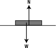
Figure 7-1. The normal contact force acting on a book resting on a table
The normal force will change if, for example, the table is tilted. You’ll see in the first example in this chapter (“Sliding down a slope”) how to calculate the normal force in such a case.
Tension and compression
Tension in strings is another contact force. If you tie an object with a piece of string and then suspend the object by holding the other end of the string (see Figure 7-2), the string exerts a pull on the object that prevents it from falling down. The string can only do this if it is taut. By Newton’s third law of motion, the object exerts an equal and opposite force on the string. The force on the string is called tension. Informally, we also refer to the force that the string exerts on the object as tension. The effect of tension on the string itself is to stretch it slightly. If the object stops moving, then the tension must be equal to the weight of the object. If the object is very heavy, the tension may stretch the string to breaking point.
![]()
Figure 7-2. Tension in a string
Springs also experience tension. Springs are designed so that large extensions are produced for relatively small tensions. Because a spring will tend to regain its normal length when stretched, it will pull back on the object that is stretching it. The opposite of tension is compression. Springs can also be compressed; they then exert a push on the object compressing them.
Springs are both great fun and extremely useful for producing a variety of effects. In fact, the next chapter is devoted exclusively to springs and spring-like motion.
Friction
Frictional forcesare forces that resist the relative movement of two bodies that are in contact or the movement of a body through a fluid. For example, if you push a book along a table, it will slow down and come to a stop. That’s because of the frictional force that the table surface exerts on it. The friction between two solid objects is also called dry friction. Fluids such as air or water also exert a frictional force, known as viscous fluid drag.
We’ll discuss fluid drag later in this chapter. In this section, we’ll look at dry friction between two solid objects and how we can model it.
As discussed, friction is a force that resists the relative motion of two objects in contact with each other. This implies that the frictional force on an object will act in a direction opposite to its motion. But an object does not necessarily have to move in order to experience friction. If an object is experiencing a force that tends to move it against another object, it can also experience friction, even if it does not actually move. In fact, it is friction that stops it from moving. So there are actually two types of friction: friction experienced by a stationary object, and friction experienced by a moving object. We call them static and kinetic friction, respectively.
Modeling static and kinetic friction
We model both types of friction using the concept of a coefficient of friction. Let’s start with kinetic friction because it is a bit simpler.
Common experience tells us that there will be more friction if we press two surfaces together while trying to slide one over the other. That’s because the two objects “stick together” more if pressed together. It’s also clear that the amount of friction will depend upon the material making up the object. Rubber, for example, would give more friction than glass. It should therefore come as no surprise to learn that the magnitude of the frictional force F is given by the following, where N is the normal force between the two objects and Ck is a number that depends on the two surfaces, known as the coefficient of kinetic friction:
![]()
By Newton’s third law, a force of the same magnitude acts on both objects; for each object, the force acts in a direction to oppose its motion relative to the other object. Kinetic friction is also sometimes referred to as dynamic or sliding friction.
Static frictionis a bit different. Whereas the kinetic frictional force has just one value for a given pair of surfaces and normal contact force, the static frictional force can take on any value up to a maximum value. The maximum value is given by the following:
![]()
This is similar in form to the formula for kinetic friction, but with a different coefficient, known as the coefficient of static friction. Its value is usually larger than the corresponding value of Ck for the same two surfaces. Hence, the maximum static frictional force is larger than the kinetic frictional force.
To understand static versus kinetic friction, consider the following thought experiment. Suppose you are pushing an object in contact with a surface. If the force you apply has a magnitude less than Fmax as given by the preceding formula, the frictional force will be equal to the applied force, so that the resultant force is zero and the object does not move. If you now push harder so that the applied force is greater than the value of Fmax, the frictional force will be equal to Fmax (because it cannot exceed that maximum value). Therefore, the frictional force cannot completely balance the applied force, and the object will begin to accelerate under the resultant force. As soon as it starts moving, the frictional force will reduce to a value equal to the magnitude of the kinetic friction. Hence, the resultant force will suddenly increase, and the object will accelerate faster. If you’ve ever tried to move a piece of heavy furniture, you will readily appreciate this fact: it is easier to push once it’s already moving. That’s because kinetic friction is less than the maximum value of static friction.
Coefficients of friction
Some examples of coefficients of friction are given in Table 7-1. The key point is that the values are generally less than 1. It is very rare for the coefficient of friction to be larger than 1, because that would imply a frictional force larger than the normal contact force holding the two objects together.
Table 7-1. Static and Kinetic Coefficients of Friction
Materials |
Cs |
Ck |
|---|---|---|
Wood on wood |
0.25–0.5 |
0.2 |
Steel on steel |
0.74 |
0.57 |
Rubber on concrete |
1.0 |
0.8 |
Glass on glass |
0.94 |
0.4 |
Ice on ice |
0.1 |
0.03 |
Note that although the values are representative of the materials cited, actual coefficients of friction may vary because of the nature of the surface of actual objects. For game programming purposes, this does not present a big problem.
It is impossible to give a comprehensive list of friction coefficients; but if what you need is not listed here it should be easy to find it online.
Example: Sliding down a slope
Time for an example! You can now apply what you learned about normal contact forces and friction to simulate an object sliding down an inclined plane. First, let’s apply the physics concepts to this particular example.
The physics
The force diagram for this simulation is shown in Figure 7-3. As indicated on the diagram, there are three forces acting on the object: gravity mg, normal contact force N, and friction f. Because the object moves in a straight line along the surface, the resultant force acts along the surface. There is no resultant force perpendicular to the surface.
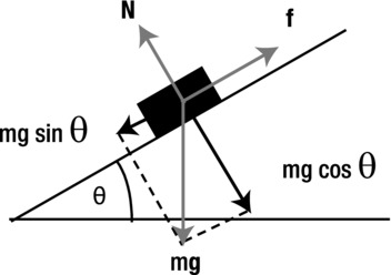
Figure 7-3. Force diagram for an object sliding down an inclined plane
Therefore, resolving the forces along the surface gives the magnitude of the resultant force F as follows, where θ is the angle of the inclined plane:
![]()
Resolving forces perpendicular to the surface must give a zero resultant, so that the normal contact force N is balanced by the component of gravity perpendicular to the surface. Note that friction f acts along the surface, so its component perpendicular to the surface is zero. Hence,
![]()
The magnitude of the frictional force f is given by the following when the object is moving:
![]()
If it is not moving, the resultant force F along the surface must be zero, so f has to balance the component of gravity along the surface. From the preceding equation, setting F = 0 gives this:
![]()
It will be true up to a maximum value of the following:
![]()
If the value of the gravity component (mg sin (θ)) exceeds this critical value (CsN), f will have the latter value, at least momentarily. As soon as the object starts moving, f will have the value CkN.
Now that you know the physics and have the relevant formulas, you can start coding. This will be a two-step process, pretty similar to what you did in the previous chapter. First, you’ll create the visual setup; then you’ll write the code that drives the simulation.
Creating the visual setup
The code is in a file called sliding.js. After declaring and initializing the canvas, context and other variables, we handle the visual setup in the init() function:
var canvas = document.getElementById('canvas'),
var context = canvas.getContext('2d'),
var canvas_bg = document.getElementById('canvas_bg'),
var context_bg = canvas_bg.getContext('2d'),

var ball;
var m = 1;          // mass of ball
var g = 10;         // acceleration due to gravity
var ck = 0.2;       // coeff of kinetic friction
var cs = 0.25;      // coeff of static friction
var vtol = 0.000001 // tolerance
// coordinates of end-points of inclined plane
var xtop = 50; var ytop = 150;
var xbot = 450; var ybot = 250;
var angle = Math.atan2(ybot-ytop,xbot-xtop); // angle of inclined plane
var t0,dt;

window.onload = init;

function init() {
     // create a ball
     ball = new Ball(20,'#0000ff',m,0,true);
     ball.pos2D = new Vector2D(50,130);
     ball.velo2D = new Vector2D(0,0);
     ball.draw(context);
     // create an inclined plane
     context_bg.strokeStyle = '#333333';
     context_bg.beginPath();
     context_bg.moveTo(xtop,ytop);
     context_bg.lineTo(xbot,ybot);
     context_bg.closePath();
     context_bg.stroke();
     // make the ball move
     t0 = new Date().getTime();
     animFrame();
};
In init() we create a ball and a line (the latter on a different canvas element, the background), and place the ball on the line. The angle of the line is calculated using the end points and the Math.atan2() function and stored in the angle variable. If you are unsure about what is happening here, take a look at the subsection “The inverse trig functions” in Chapter 3 again. Finally, we make the ball move down the inclined line by invoking the animFrame() function.
Coding the animation
The animFrame() function does its usual job of setting up the animation loop, and the relevant code is very much like the examples in the previous chapter, but just to remind you we reproduce the code here:
function animFrame(){
     animId = requestAnimationFrame(animFrame,canvas);
     onTimer();
}
function onTimer(){
     var t1 = new Date().getTime();
     dt = 0.001*(t1-t0);
     t0 = t1;
     if (dt>0.2) {dt=0;};
     move();
}
function move(){
     moveObject(ball);
     calcForce();
     updateAccel();
     updateVelo(ball);
}
function moveObject(obj){
     obj.pos2D = obj.pos2D.addScaled(obj.velo2D,dt);
     context.clearRect(0, 0, canvas.width, canvas.height);
     obj.draw(context);
}
function updateAccel(){
     acc = force.multiply(1/m);
}
function updateVelo(obj){
     obj.velo2D = obj.velo2D.addScaled(acc,dt);
}
This is almost the entire animation code, and you can see that nothing has changed so far. The only change is in the calcForce() function, which contains the new physics:
function calcForce(){
     var gravity = Forces.constantGravity(m,g);
     var normal = Vector2D.vector2D(m*g*Math.cos(angle),0.5*Math.PI-angle,false);
     var coeff;
     if (ball.velo2D.length() < vtol){  // static friction
          coeff = Math.min(cs*normal.length(),m*g*Math.sin(angle));
     }else{  // kinetic friction
          coeff = ck*normal.length();
     }
     var friction = normal.perp(coeff);
     force = Forces.add([gravity, normal, friction]);
}
The calcForce() method calculates the three relevant forces gravity, normal, and friction at each timestep and then adds them up to get the resultant force by using the Forces.add() method. The calculation of the normal and friction forces requires explanation. For the normal force, we are using a new method of Vector2D called vector2D(), which is defined as follows:
Vector2D.vector2D = function(mag,angle,clockwise){
     if (typeof(clockwise)==='undefined') clockwise = true;
     var vec = new Vector2D(0,0);
     vec.x = mag*Math.cos(angle);
     vec.y = mag*Math.sin(angle);
     if (!clockwise){
          vec.y *= -1;
     }
     return vec;
}
This method takes two required Number arguments, mag and angle (in radians), and an optional Boolean argument clockwise, and returns a Vector2D object which is a 2D vector with the specified magnitude and angle. It does this by converting from the (magnitude, angle) representation to the component representation of a vector (refer to the section “Resolving vectors,” in Chapter 3). The clockwise parameter tells vector2D() whether the angle is taken in a clockwise direction (the default) or in a counterclockwise direction.
Using the previous formulas and Figure 7-3, we know that the magnitude of the normal force is equal to mg cos (θ), and its angle is equal to π/2 – θ (that’s 90° – θ, in radians) taken in an anticlockwise sense. Therefore, the normal force is given by this:
var normal = Vector2D.vector2D(m*g*Math.cos(angle),0.5*Math.PI-angle,false);
The friction force is perpendicular to the normal force and has a magnitude of coeff*N, where coeff is the coefficient of friction and N is the magnitude of the normal force. It is therefore given by the following, where perp() is another new method we created in the Vector2D class (which we shall describe shortly) and coeff is equal to CkN when the object starts moving; and is equal to mg sin (θ), up to a maximum of CsN, when the object is not moving:
var friction = normal.perp(coeff);
This is implemented in the following way:
if (ball.velo2D.length() < vtol){  // static friction
     coeff = Math.min(cs*normal.length(),m*g*Math.sin(angle));
}else{  // kinetic friction
     coeff = ck*normal.length();
}
Note that we make use of the Math.min() function to implement the fact that for static friction, coeff is equal to either mg sin (θ), or CsN, whichever is smaller.
The perp() method of Vector2D is defined like this:
Function perp(u,anticlockwise){
     if (typeof(anticlockwise)==='undefined') anticlockwise = true;
     var length = this.length();
     var vec = new Vector2D(this.y, -this.x);
     if (length > 0) {
          if (anticlockwise){ // anticlockwise with respect to canvas coordinate system
               vec.scaleBy(u/length);
          }else{
               vec.scaleBy(-u/length);
          }
     }else{
          vec = new Vector2D(0,0);
     }
     return vec;
}
This definition implies that if vec is a Vector2D object, and k is a number, vec.perp(k) returns a Vector2D object that is perpendicular to vec and of length k, with a counterclockwise orientation to vec (in the canvas coordinate system). Referring to Figure 7-4, which shows a screenshot of the setup, normal.perp(coeff) therefore gives a vector of magnitude coeff directed up the slope, just as the frictional force should be.
Figure 7-4. An object sliding down a slope
When checking to see if the object is not moving, we don’t actually check that its velocity is zero but that it’s smaller than some small value vtol (set at 0.000001 in the code). The value of g is set at 10 and, assuming both the sliding object and the surface are made of wood, we choose ck = 0.2 and cs = 0.25.
If you run the code with the given choice of values for the parameters, you’ll see that nothing happens. The object just stays there. How can this be? To understand this, take another look at Figure 7-3. It is clear that the object can slide only if the component of gravity along the slope exceeds the maximum static friction. In other words, it will slide if the following condition is true:
![]()
Because N = mg cos (θ), this is equivalent to the following:
![]()
Dividing both sides of this inequality by mg cos (θ) gives this:
![]()
So the object will slide only if the tangent of the slope angle is greater than the coefficient of static friction.
Now you can calculate tan (θ) from the values of xtop, ytop, xbot, and ybot as follows:
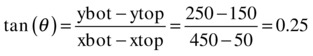
This is exactly equal to the value of Cs specified in the code. Therefore, gravity is not sufficient to overcome the force of friction, and the object does not slide. If you increase the angle of the slope slightly, the object will slide. For example, if you change the value of ybot to 260, this will give tan (θ) = 110/400 = 0.275, which is larger than the value of Cs. Give it a go!
In this example, the object slides along a surface without rolling. Rolling involves rotational motion of a rigid body (it will be discussed in Chapter 13).
The rest of this chapter will deal with forces that originate from pressure, more specifically fluid pressure. Technically, pressure is associated with solids as well as liquids and gases. But the concept is especially useful in relation to fluids, so it tends to be associated more with liquids and gases.
The meaning of pressure
So what is pressure? It is the normal (perpendicular) force per unit area exerted on the surface of an object. The origin of that perpendicular force can be different in different cases. Pressure due to solids and liquids is usually due to the force of gravity. Pressure in gases is due to collisions by gas molecules.
The key question is this: how can we calculate pressure and thus the forces on an object in a fluid? Once we can do that, we can try to simulate the motion of an object in a fluid.
Based on this definition of pressure, if a force F acts normally to a surface with area A, the average pressure P on the surface is given by the following:

Because pressure is force divided by area, its unit is N/m2. This unit has a special name: the pascal, or Pa.
What if F acts at an angle to the normal? Then you need to resolve F to find the component along the normal, and that normal component is what you use in the preceding formula. This gives us a method for calculating the pressure if we know the force, and vice versa.
Pressure is not restricted to fluids (although fluid pressure will be our main concern in this chapter), and it is actually easier to introduce the method of calculating pressure using a simple illustrative example of a solid object.
Suppose that a cuboid (box) of length l, width w, height h, and mass m sits on a table (see Figure 7-5). What is the pressure it exerts on the table?
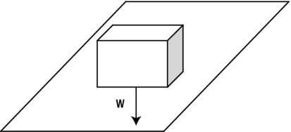
Figure 7-5. A box sitting on a table
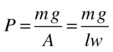
The force it exerts on the table is equal to its weight, and that force is perpendicular to the table surface, so we have F = mg. The area A = lw. Hence, the pressure P is given by this:
We can make some more progress by introducing the concept of density.
Density is defined as mass per unit volume. Density gives you a way of comparing the relative “heaviness” of different substances—you can take the same volume of each substance and compare how much each weighs.
We use the Greek symbol ρ (rho) for density. So, based on the definition, we can write:

Because density is a mass divided by a volume, its unit is kg/m3. Because things expand when heated, especially liquids and gases, the density of a fluid varies with temperature (and also with pressure). At 20°C and standard atmospheric pressure, the density of water is approximately 1000 kg/m3, and that of air is approximately 1.2 kg/m3. That means a box measuring 1m × 1m × 1m (of volume 1 m3) would hold 1000 kg (1 ton) of water and 1.2 kg of air.
Manipulating the above formula gives this:
![]()
It also gives this:

We’ll use these formulas frequently in the rest of this chapter.
Just like pressure, the concept of density applies to solids as well as liquids. Going back to the preceding illustrative example of the cuboid, we can replace the mass m in the formula for pressure by using m = ρV = ρlwh because the volume of the cuboid is V = lwh:
This is a very useful formula. It gives the pressure exerted by a regular object (in this case, a cuboid) on a surface in terms of three known quantities: the density of the object, the acceleration due to gravity, and the height of the object. Note that we could have used another shape other than a box, as long as it had a regular cross-section A. The area A would cancel out in the same way, leaving the same formula: P = ρgh.
In the next section, we’ll find that this formula is actually even more general, and also applies to the pressure exerted by fluids, provided that we reinterpret h.
Variation of pressure with depth in a fluid
Instead of a solid, now consider a column of liquid of the same shape as the solid in the last section.
Exactly the same math applies, and we again end up with the following, where P is the pressure underneath the column of fluid, ρ is the density of the fluid, and h is the height of the fluid column:
![]()
Now mentally transport yourself to the ocean.
At a depth h beneath the sea surface, there is a column of water of height h above. Hence, the pressure at depth h below the surface is given by the same formula:
![]()
Note that this is the pressure due to the water only. There is also an additional pressure due to the air above the water surface. This is atmospheric pressure, which we can denote by A. Then the total pressure at a depth h in the ocean is A + ρgh, assuming the density of water is constant with depth. This formula shows that pressure in a fluid increases with depth, which makes perfect sense because there is more fluid above that is “weighing down.”
The same is true in the atmosphere, too. The air pressure we feel at the surface of the Earth is due to the column of air above our heads. Standard atmospheric pressure is approximately 100 kPa, or 100,000 Pa. This is sometimes simply called 1 atmosphere (atm).
Because the density of water is 1000 kg/m3, and g is approximately 10 m/s2, using the formula P = ρgh tells us that 10 m of water will exert approximately the same pressure as 1 atm. So, at an ocean depth of 10 m, the pressure will be 2 atm, including the pressure of the air above.
Static and dynamic pressure
So far, when we’ve talked about pressure in a fluid, we’ve been referring to static pressure. The formula P = ρgh applies to static pressure. Static pressure is defined at any point in a flow, and it is isotropic; that is, it has the same value in any direction. It exists even in static fluids (fluids that are at rest).
In a moving fluid, there is another kind of pressure, known as dynamic pressure. Dynamic pressure is due to the flow of fluid. For example, the flow of water from a tap gives rise to dynamic pressure. When the water hits the sink, it exerts a force on the sink. Similarly, the wind exerts a force due to the dynamic pressure associated with it. The formula for the dynamic pressure at any point in a fluid is the following, where v is the velocity of the fluid at that point:

The same is true for an object moving with velocity v in a fluid; it’s the relative velocity between the object and the fluid that matters.
The total pressure in a moving fluid is the sum of the static and the dynamic pressure.
Upthrust (buoyancy)
After this background on pressure and density, we are now ready to introduce the forces due to fluids. So let’s start with upthrust, also known as buoyancy.
Here is a simple experiment for you to do in the bath. Try pushing a hollow ball under water. What do you feel? You should feel a force trying to push the ball back upward. This is the upthrust force. Now let go of the ball. What happens? It pops back up and oscillates at the water surface before settling down. You will create such an effect soon.
Upthrust is also responsible for making us feel lighter in the swimming pool or bath. It acts upward, opposing the force of gravity.
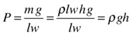
What causes upthrust? The physical origin of upthrust is the difference in pressure that exists at different heights in a fluid. To see what we mean, take a look at Figure 7-6a, which shows an object partially immersed in a fluid such as water. The pressure on the top face of the object is equal to atmospheric pressure A and pushes the object downward, while the pressure on the bottom surface is equal to A + ρgh, where ρ is the density of the fluid and h is the depth to which the object is submerged. This pressure acts upward, so that there is a net upward pressure equal to ρgh. Hence, because force = pressure × surface area, there is a resultant upward force U due to this pressure difference given by the following (where S is the area of the top and bottom faces of the object—assumed to be equal here for simplicity):
![]()
This is the upthrust or buoyancy force.
Note that because pressure is isotropic, it also acts on the sides of the object. But the pressures on opposite sides are equal and opposite at each height, so their effects are cancelled. Similar conclusions hold if the object is completely immersed in a fluid (see Figure 7-6b), including objects in air. That’s basically because pressure increases with depth in a fluid, so the pressure at the base of a submerged object will always be greater than that at its top. So there will be a net upward pressure on the object due to the fluid.
Figure 7-6. An object immersed in a fluid experiences upthrust due to a pressure difference
Let’s revisit the last formula we derived in the preceding section. The magnitude of the upthrust U was found to be given by U = ρghS. Now h is the height of the submerged portion of the object and S is its cross-sectional area (which we assume to be constant for simplicity). Hence, hS is equal to the volume V of the submerged portion of the object. So we can write this:
![]()
But then ρV = m, the mass of the fluid whose place has been taken by the submerged portion of the object, so we can now write this:
![]()
This is just the weight of the displaced fluid. Hence, we have derived Archimedes’ principle:
- Archimedes’ principle: The upthrust on an object immersed in a fluid is equal to the weight of fluid it displaces.
Archimedes was an ancient Greek scientist, mathematician, and all-round genius. According to legend, upon discovering this principle, he jumped out of his bath shouting “Eureka!”, which means “Found it!”
Apparent weight
Upthrust leads to the phenomenon of apparent weight. Figure 7-7 illustrates the concept. Any object that is partially or completely immersed in a fluid will experience an upward upthrust force U that opposes the downward force of gravity W on it.
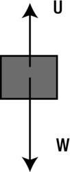
Figure 7-7. Upthrust reduces the apparent weight of an object to W – U
Hence, the apparent weight of the object is given by
![]()
The phenomenon of apparent weight is responsible for why we feel lighter in the bath or a swimming pool. Exploiting the apparent weight effect, astronauts train while submerged in a giant water tank to simulate reduced or zero gravity.
Submerged objects
Objects that are completely immersed (submerged) in a fluid obviously displace their own volume of fluid.
The apparent weight of a completely immersed object can therefore be written as follows because both the object and the displaced fluid have the same volume V:
![]()
It can therefore be written in the following form:
![]()
This is a very useful formula that gives the resultant downward force, or apparent weight, of an object submerged in a fluid in terms of their densities and the volume of the submerged object.
From this formula, we can deduce:
- If the density of the object is greater than that of the fluid, the apparent weight will be positive (i.e. downward) but less than the real weight. You can experience this lower apparent weight in the bath or a swimming pool.
- If the density of the object is much greater than that of the fluid, the apparent weight is nearly equal to the real weight because the upthrust is negligible compared to the weight of the object. For example, the upthrust on a stone in air can usually be neglected.
- If the density of the object is exactly equal to that of the fluid, the apparent weight will be zero, and so the object will float in the fluid.
- If the density of the object is less than that of the fluid, the apparent weight is negative (it acts upward) and so the object will rise. For example, air bubbles in water have a very large upthrust compared with their weight because the density of air is much lower than that of water, and so they rise quickly.
Floating objects
A special form of Archimedes’ principle applies for floating bodies. This is the so-called law of flotation.
- Law of flotation: A floating object displaces its own weight of fluid.
Here’s the logic. A floating body has no net force acting on it; otherwise, it would either rise or sink. Because the only two forces acting on it are its weight and upthrust, they must balance. Hence, the upthrust on a floating body must equal the weight of the body. By Archimedes’ principle, this implies that the weight of fluid displaced is equal to the weight of the body. So the apparent weight of a floating object is zero—it “feels weightless.”
As discussed previously, this is also the situation when a body is submerged in a fluid with a density equal to the body’s own density. In fact, an object that is floating on the surface of a liquid, such as a ship on water, has an “effective density” that is the same as that of the water, even though it may be made of metal with a higher density than that of water. That’s because the part of the ship below the water surface also includes air enclosed within the ship’s interior, which lowers its average density.
Example: Balloon
We’ve had quite a bit of theory, so let’s look at an example. This example (shown in Figure 7-8) simulates a simple hot-air balloon. Hot-air balloons work, well, by heating air. The heated air has a density less than that of the ambient air, so it rises. By controlling the temperature of the air in the balloon, you can control its density and therefore the upthrust on it.
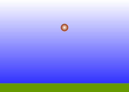
Figure 7-8. Simulating a hot-air balloon
The code for this simulation is found in balloon.js. The init() function creates the visual background shown in Figure 7-8 and creates a balloon as a Ball object, initially at rest on the ground. It also sets up keydown and keyup event listeners, with the corresponding keydown event listener responding to UP and DOWN arrow presses by respectively increasing or decreasing the balloon’s density rhoP from its initial value of 1.1. The air density rho is kept constant at 1.2. You can take a look at the code for more details.
You could probably write the animation code without too much help by now. The only substantial change here is the calcForce() method, which specifies two forces (gravity and upthrust) and then adds them up:
function calcForce(){
     var gravity = Forces.constantGravity(m,g);
     var V = m/rhoP; // volume of air displaced
     var upthrust = Forces.upthrust(rho,V,g);
     force = Forces.add([gravity, upthrust]);
}
The upthrust is calculated using the newly created Forces.upthrust() static function, which basically uses the formula U = ρgV, where ρ (variable rho) in the code is the density of the fluid and V (variable V in the code) is the volume of air displaced. This is the volume of the balloon because it is completely immersed in air. So V is calculated using the mass of the balloon and its effective density rhoP, using the formula volume = mass/density. The effective density rhoP is the density of the whole balloon, including any load it carries (not just the density of the air in it).
The critical parameter in the simulation is the ratio of the balloon density to ambient air density rhoP/rho. If the effective balloon density rhoP is smaller than the air density rho (that ratio is smaller than 1), the balloon will rise. If rhoP is larger than rho, it will sink.
To make the simulation more interactive, we’ve also included a call in move() to the function changeBalloonDensity() that lets you increase and decrease the density rhoP of the balloon by pressing the up and down arrow keys, respectively. The code outputs the value of the ratio (rhoP/rho) to the console whenever rhoP is changed. See if you can make the balloon rise and then remain stationary at some height.
There is something missing in this simulation. The balloon rises too fast; it basically accelerates under the effect of the excess upthrust force, so its upward velocity keeps on rising. In reality, it will be slowed down by drag. So let’s take a look at how we can include drag effects.
Trying to model drag can prove somewhat confusing for someone who is not familiar with fluid dynamics. One reason is that there is not just one, but several types of drag. Depending on the object and flow you are simulating, you might need to consider different types of drag.
Another source of difficulty is that a lot of what we know about drag is based on empirical work. The laws of drag were discovered by doing lots of experiments, and not as part of a beautiful universal theory like gravity.
The bottom line is that you will bump into formulas that were developed from experimental results that you just have to accept without argument.
For most of what we’ll do in this book, we’ll use one of two drag laws: one that holds for low velocities (or so-called laminar flow) and another (more common) one that holds for higher velocities (or so-called turbulent flow).
Drag law for low velocities
For an object moving through a fluid at very low velocities, the flow around the object is laminar, or streamlined. This generates relatively low drag. The drag force then obeys Stokes’ law, which says that the drag force is proportional to the velocity of the object. For a spherical object, the Stokes’ drag formula is the following, where r is the radius of the sphere and the Greek letter η denotes a property of the fluid known as viscosity (more precisely, dynamic viscosity):
![]()
Note that dynamic viscosity is also denoted by the Greek letter μ. The viscosity of a fluid is a measure of the resistance it offers to objects moving through it. Intuitively, it represents the “thickness” of the fluid. So the viscosity of water is higher than that of air, and the viscosity of oil is higher than that of water. Therefore, an object moving at the same velocity through water experiences a greater drag force than through air. The formula also tells us that a larger object experiences more drag because the parameter r is greater for a larger object.
To use this formula in an accurate simulation, you need to know the viscosity of the fluid in which your object is moving. Like density, viscosity depends on temperature. At 20°C, the dynamic viscosity of water is 1.0 × 10⁻³ kg/(ms), and that of air is 1.8 × 10⁻⁵ kg/(ms)—about 1/55 as much.
In coding this drag force, we will lump together all the factors, multiplying the velocity into a single factor denoted by k, so that the linear drag law becomes the following, where k = 6πηr for a sphere:
![]()
Writing the linear drag law in this form is in fact more general because it then also applies to other, nonspherical objects, for which k is not given by this formula. By choosing suitable values for k, we can model the linear drag force on objects of any shape.
This is basically the form of drag that we coded into the Forces.linearDrag() function back in Chapter 5:
Forces.linearDrag = function(k,vel){
     var force;
     var velMag = vel.length();
     if (velMag > 0) {
          force = vel.multiply(-k);
     }else {
          force = new Vector2D(0,0);
     }
     return force;
}
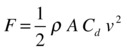
Drag law for high velocities
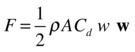
Stokes’ drag law holds only for low velocities. At higher velocities, the flow around the immersed object becomes turbulent, generating eddies that disturb the flow and make it chaotic. The drag force law is then different from that of laminar flow and is proportional to the square of the velocity of the object. The drag formula is given by the following, where ρ is the density of the fluid, A is the frontal area of the object (the area on which the fluid impacts as the object moves through it), and Cd is a parameter called the drag coefficient, which depends on characteristics of the object such as its shape, surface properties, and characteristics of the flow:
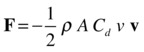
Note that the formula involves the product of the velocity v with its magnitude v. This gives a vector of magnitude v2 in the direction of v. Hence, the drag force law is quadratic in the velocity, with a magnitude given by this:
In this form, it is clear that quadratic drag depends on dynamic pressure P = 1/2 ρv2, and indeed we can write this:
![]()
As mentioned previously, the drag coefficient Cd can depend on a large number of factors. Its value is found by experiment for particular objects and setups. For example, the drag coefficient of a sphere can range from 0.07 to 0.5. Similarly, you can find the drag coefficients for a large number of object shapes (both in 2D and in 3D) in physics or engineering textbooks or websites.
As for the laminar drag formula, we’ll simplify the previous formula by defining a drag constant k for high velocities as the following:
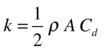
So the drag law for high velocities can be written in this form:
![]()
We now define a second drag force function called Forces.drag(), which looks as follows:
Forces.drag = function(k,vel) {
     var force;
     var velMag = vel.length();
     if (velMag > 0) {
          force = vel.multiply(-k*velMag);
     }
     else {
          force = new Vector2D(0,0);
     }
     return force;
}
Which drag law should I use?
We have described two drag laws, linear and quadratic, saying the former applies at low velocities and the latter at high velocities. But so far we’ve been rather vague about what “low” and “high” mean. What is the “critical velocity” that distinguishes between low and high?
To answer this question, we introduce the concept of the Reynolds number of a flow. In simple terms, the Reynolds number tells us whether a flow is laminar or turbulent. Therefore it tells us, among other things, whether a linear or a quadratic drag law applies. The Reynolds number, denoted by the symbol Re, is defined by the following equation, where u is a characteristic velocity associated with the flow, d is a characteristic length scale, and the Greek symbol ν (nu) is the so-called kinematic viscosity of the fluid:

The kinematic viscosity is defined as the ratio of the dynamic viscosity and the density of the fluid:

Using the values of dynamic viscosity and density given before, we can deduce that at 20°C the kinematic viscosity of water is 1.0 × 10⁻⁶ m2/s and that of air is 1.5 × 10⁻⁵ m2/s.
The choice of what velocity u and what length scale d to use to calculate the Reynolds number depends on the problem. For an object such as a sphere moving in a fluid, u is just the velocity of the object and d is a linear dimension (the diameter for a sphere).
Now it is found experimentally that laminar flow dominates, and therefore Stokes’ law for linear drag holds when the Reynolds number is much less than 1. Using the formula for the Reynolds number and setting Re = 1, this implies that the critical velocity that determines which drag law applies is given by

If the velocity of the object is much less than this critical value vc, the drag law is linear; if it is much larger than vc, the drag law is quadratic. If the velocity is intermediate between those two limits, a combination of both laws can be used.
As an example, the diameter of a soccer ball is 22 cm, or 0.22 m. Using the values of the kinematic viscosity of water and air given previously, we deduce that the critical velocity for such a ball is 0.0045 mm/s in water and 0.068 mm/s in air (yes, those are in millimeters per second). These are tiny velocities, so for all practical purposes you can assume that a ball this size moving in water or air will always obey a quadratic drag law. This also applies to most everyday objects moving at normal velocities in air or water.
On the other hand, a ball bearing of diameter 1 mm falling in glycerin (which has a kinematic viscosity of 1.2 × 10⁻³ m2/s at 20°C) has a critical velocity of 1.2 m/s. That’s a much greater critical velocity. The maximum velocity that the ball bearing reaches (its terminal velocity) is much less than this. Therefore, the linear drag law applies in this case.
Adding drag to the balloon simulation
As shown in the previous section, the drag law that is appropriate for most everyday objects moving in air or water is the quadratic drag law, as coded in the Forces.drag() function. It is a very simple matter to add drag to the last example of the balloon simulation. We simply update calcForce() as follows:
function calcForce(){
     var gravity = Forces.constantGravity(m,g);
     var V = m/rhoP; // volume of air displaced
     var upthrust = Forces.upthrust(rho,V,g);
     var drag = Forces.drag(k,balloon.velo2D);
     force = Forces.add([gravity, upthrust, drag]);
}
The new variable k is the drag constant. In the sample code provided, we give it the value of 0.01. If you run the simulation with these modifications, you’ll see that the balloon no longer rises at an accelerating rate. The addition of the drag force slows down its ascent, and the effect is more realistic.
Example: Floating ball
Let’s now go back to the floating ball simulation we introduced in Chapter 5 to illustrate the effect of drag, together with upthrust and gravity. The code simulates the motion of a ball that is thrown, dropped, or released in water.
The code is in the file floating-ball.js. The visual and interactive aspects of the code were discussed in Chapter 5. Here we’ll focus on the physics, which is essentially contained in the calcForce() method:
function calcForce(){
     var rball = ball.radius;
     var xball = ball.x;
     var yball = ball.y;
     var dr = (yball-yLevel)/rball;
     var ratio;                            // volume fraction of object that is submerged
     if (dr <= -1){                        // object completely out of water
          ratio = 0;
     }else if (dr < 1){                    // object partially in water
          //ratio = 0.5 + 0.5*dr;          // for cuboid
          ratio = 0.5 + 0.25*dr*(3-dr*dr); // for sphere
     }else{                                // object completely in water
          ratio = 1;
     }
     var gravity = Forces.constantGravity(ball.mass,g);
     var upthrust = new Vector2D(0,-rho*V*ratio*g);
     var drag = ball.velo2D.multiply(-ratio*k*ball.velo2D.length());
     force = Forces.add([gravity, upthrust, drag]);
     // bouncing off walls
     if (xball < rball){
          ball.xpos = rball;
          ball.vx *= vfac;
     }
     if (xball > canvas.width - rball){
          ball.xpos = canvas.width - rball;
          ball.vx *= vfac;
     }
}
The section of code consisting of the two if blocks at the end of calcForce() handles bouncing of the ball off the walls. The four lines of the code before that should be evident: we are calculating the three forces (gravity, upthrust, and drag) that act on the ball and then adding them up to obtain the resultant force. The new piece of physics here is the inclusion of a factor called ratio, which is the fraction by volume of the ball that is submerged in the water. This is used to compute the upthrust in the water (according to Archimedes’ principle), and the drag in the water (assuming that this is also proportional to the volume fraction that is submerged—it is actually a fairly crude approximation, but will help keep the algorithm much simpler). For simplicity, we neglect the upthrust and drag forces that the ball might experience in air. It is not difficult to see how they could be included too, if needed. All this should be easy to follow; the subtlety is in the code that calculates ratio.
To calculate ratio, you need to do some geometrical thinking. Take a look at Figure 7-9, which represents a cuboid and a sphere partially immersed in water. In our animation, assuming that coordinates of the corresponding objects are at the center of the objects, we need a formula that gives ratio in terms of the position of the objects and the position of the water level.
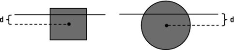
Figure 7-9. Objects partially immersed in water
To do this, it turns out to be convenient to first define a parameter dr that tells you how much the center of the object is above or below the water level, as a fraction of the radius of the ball (or half-height of the cuboid). So dr is defined as the following, where r is the half-height of the object (and is equal to the radius for the ball):
![]()
A little bit of thinking should convince you that dr = –1 means that the object (whether ball or cuboid) is just completely out of the water, and that dr = 1 means that it is just completely submerged in the water. Therefore, if dr <= –1, ratio is zero, and if dr >= 1, ratio is 1. The trickier part is when the object is partially submerged. In the case of a cuboid, simple geometry tells us that (yes, you can work it out yourself):ratio = 0.5 + 0.5 dr
![]()
In the case of a sphere, it’s a bit more complicated to work out (you need to do a bit of calculus), but here is the formula:ratio = 0.5 + 0.25 dr (3 − dr2)
![]()
That’s all we need.
In the code, the volume V of the ball is set to 1, and its mass is also 1. Therefore, its density (equal to mass/volume) is 1. The density of the water is set to 1.5. Therefore, because the density of the ball is less than that of the water, it will float.
In floating-ball.js, the initial position and velocity of the ball are given as follows:
ball.pos2D = new Vector2D(50,50);
ball.velo2D = new Vector2D(40,-20);
This puts the ball initially above the water and imparts a velocity with an upward component and a component to the right. If you run the code, you’ll see that the ball then follows a curved (parabolic) path in the air until it hits the water. It then slows down suddenly because of the drag and upthrust in the water, sinking a bit and then rising again to the surface and oscillating on the water surface until it stops. A screenshot of the simulation is shown in Figure 7-10.
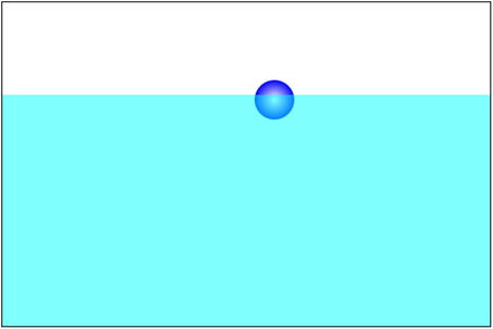
Figure 7-10. A floating ball
The simulation is so realistic that you can experiment with it to learn about the physics involved! Click anywhere above the water to move the ball there. Then release it above the water. It will fall into the water, decelerate, rise, and again oscillate on the water surface a few times before stopping. The higher you drop it, the further it will sink. Now click underwater and release it. It will rise to the surface and again oscillate a few times before stopping.
You can also play around by changing the initial conditions or the values of the parameters. For example, change the mass of the ball to 2 or the volume to 0.5, so that the density is 2. The ball will then sink instead of floating because its density is greater than the density of the water, which is 1.5.
Want to try something different? What would happen if the ball were very light? Try it. Reduce the density to 0.5 by increasing the volume to 2. What happens when you release the ball under water? It shoots out into the air, before falling back into the water. If you’ve ever tried doing this with a real ball, you’ll know that it’s a real effect. Our simulation is so realistic it can be used to perform “virtual experiments”. And we haven’t even paid any attention to numerical accuracy (which we’ll look at in Part IV of the book).
This example is particularly instructive in that it shows how a simulation that includes the relevant physics can behave pretty much like the real thing would do in real life. The simulation knows how to deal with any change in initial conditions or parameters, without the need for you to tell it anything more! This is the power of real physics simulation. It gives you a lot for your money, perhaps more than you’d expect—and it’s much easier than faking it!
Terminal velocity
As you discovered in the preceding examples, the presence of the drag force means that the velocity of a rising or falling object cannot increase indefinitely. To understand why, consider the case of an object released from a height (far from the ground) and falling under gravity. This example was discussed in Chapter 4 and elaborated upon in Chapter 5, but it is worth a recap here to gain a deeper understanding, now that you know more about the drag force. In particular, the previous discussions were in terms of the linear drag formula; it is useful to know how the results generalize to quadratic drag, and also when upthrust is taken into account.
In Figure 7-11, there is a downward gravity force W = mg acting on the object, and an upward drag force D. The drag force has a magnitude given by kv at very low velocities but more usually by kv2. Now initially the velocity of the object is zero, so that the drag force is zero. As it accelerates under gravity, its velocity increases and therefore the drag force increases, too. This reduces the resultant downward force to W – D and therefore reduces the acceleration. Because the force of gravity is constant, as the velocity increases, there will be a point at which the drag force will be equal to gravity; in other words, the resultant force W – D will be zero, so the acceleration of the object will be zero. In other words, it will eventually move at a constant velocity: the terminal velocity.
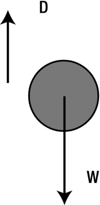
Figure 7-11. Force balance giving rise to terminal velocity
As shown in Chapter 4, it is easy to work out the magnitude of the terminal velocity. It is the value of v at which W – D = 0. Because W = mg, if we use D = kv, we get this:
![]()
So that

This is the terminal velocity for laminar flow. It holds for an object moving in a fluid with high viscosity (such as oil).
If we use the drag law for higher velocities, D = kv2, we instead get
![]()
It then implies that

We can also generalize these formulas to include upthrust (see Figure 7-12) by replacing the weight W = mg by the absolute value of the apparent weight Wapparent = (ρobject – ρfluid) V g.
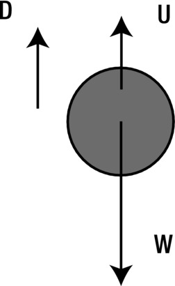
Figure 7-12. Force balance with upthrust
If you are doing a simulation in which the object attains terminal velocity very quickly, you may get away with just giving the object a constant velocity equal to the terminal velocity by making use of the preceding formulas. This will preserve the physical realism of the simulation (if the initial acceleration is not important) while cutting down the computing time significantly. For example, bubbles rising in water attain terminal velocity very rapidly and can be simulated in this way if there are no other forces apart from gravity, upthrust, and drag.
As discussed in Chapter 5, the motion of an object under gravity, upthrust, and drag can be solved analytically using calculus to give not only the terminal velocity but also the velocity at any time. For example, for an object dropped from rest in a fluid, the analytical solution assuming linear drag and neglecting upthrust is given by
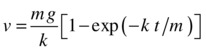
This gives the velocity of the object at time t after being dropped. The solutions with quadratic drag and including upthrust look a bit more complicated, and you can find them in physics textbooks.
Example: Parachute
Parachutes work by exploiting the fact that the drag force is proportional to the area of an object. Going back to the formula for quadratic drag F = –kvv, with the drag constant k given by k = 1/2 ρACd, we can see that the larger the area of an object, the greater the drag force will be. Opening a parachute suddenly increases the surface area exposed to the air, thereby increasing the value of k. This greatly increases the drag force and therefore slows down a parachutist.
Our present example is an educational exercise to illustrate this principle. Take a look at the init() function in parachute.js:
function init() {
     ball = new Ball(20,'#0000ff',m);
     ball.pos2D = new Vector2D(650,50);
     ball.velo2D=new Vector2D(0,0);
     ball.draw(context);
     setupGraph();
     window.addEventListener('mousedown',openParachute,false);
     t0 = new Date().getTime();
     t = 0;
     animFrame();
};
This simply creates a Ball instance (to represent a skydiver!) and then animates its fall in the usual way through animFrame() and related motion code. The calcForce() method adds gravity, upthrust, and drag:
function calcForce(){
     var gravity = Forces.constantGravity(m,g);
     var drag = Forces.drag(k,ball.velo2D);
     var upthrust = Forces.upthrust(rho,V,g);
     force = Forces.add([gravity, upthrust, drag]);
}
In addition, an event listener is set up in init() for a mousedown event. In the corresponding event handler openParachute(), the radius of the parachute is increased by a factor equal to linearFactor (which is given the value of 3 in the code), and the value of the drag constant k is increased by a factor equal to the square of linearFactor (by 9). The event listener is then removed.
function openParachute(evt){
     k *= linearFactor*linearFactor;
     ball.radius *= linearFactor;
     window.removeEventListener('mousedown',openParachute,false);
}
This means that the parachute is made three times bigger (by radius) and the drag constant is made nine times greater the first time the user clicks the mouse. Finally, a Graph object is set up in setupGraph(), which is called in the init() function, and used to plot the vy component of the parachute’s velocity at each time by calling the plotGraph() method within the move() method.
If you now run the code (without opening the parachute) you’ll find that the parachute accelerates quickly at first, then more slowly until it reaches a constant velocity (terminal velocity) about 10 seconds into the fall. The value of the terminal velocity is approximately 30 pixels per second. If you then click to “open the parachute,” it will become bigger and immediately slow down, reaching a new lower terminal velocity of approximately 10 pixels per second in a few seconds. The terminal velocity is the same whenever you open the parachute: it’s independent of time, only depending on the mass m of the parachute, the acceleration due to gravity g, and the drag constant k through the formula ![]() . Figure 7-13 shows a typical shape of the velocity-time graph.
. Figure 7-13 shows a typical shape of the velocity-time graph.
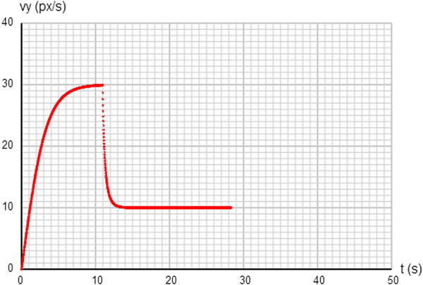
Figure 7-13. Velocity-time graph for a parachute
Lift
You saw that the drag force depends upon the dynamic pressure. There is another force that also depends on the dynamic pressure: it’s called lift. More precisely, it is the difference in dynamic pressure on opposite sides of an object that is responsible for these forces. Whereas the drag force on an object acts opposite to the velocity of the object, the lift force acts perpendicular to the velocity (see Figure 7-14). Now, because there is always a difference in the dynamic pressure between the front and back of a moving object, there is always a drag force on a moving object. However, if an object is perfectly symmetrical along an axis in the direction of motion, the flow (and therefore the dynamic pressure) on either side of the object will be exactly the same. In that case, there is no lift force. But any asymmetry in the flow—for example, caused by an asymmetrical wing shape (for aircraft) or angle of attack, will give rise to a lift force perpendicular to the direction of motion.
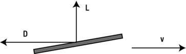
Figure 7-14. Drag and lift force on an object moving in a fluid
The lift force is what enables airplanes to fly. In that case, the direction of motion is usually horizontal, so the lift force acts vertically upward and balances the weight of the plane. But lift does not always have to act vertically upward. Depending on the direction of motion, it can act in any direction.
Lift is sometimes confused with upthrust. In fact, upthrust is sometimes mistakenly referred to as lift. Like upthrust, lift arises because of a difference in pressure. Upthrust is caused by the difference in static pressure between the top and bottom of an object that is due to the weight of the displaced fluid (buoyancy); but lift is caused by the difference in dynamic pressure between opposite sides of an object that lie along the direction of its motion. This causes a difference in the static pressure between the opposite sides mentioned earlier. Thus, whereas upthrust is always upward (as its name suggests), that is not necessarily so for lift. More crucially, the physics laws and therefore the formulas that govern these two forces are completely different. Consider this: lift is the force that makes an airplane fly; upthrust is the force that makes a balloon float; the mechanisms are different in the two cases.
Lift coefficients
The lift force is modeled in terms of a lift coefficient, in exactly the same way as quadratic drag. Hence the magnitude of the lift force can be written as follows, where CL is the lift coefficient and A is the area of the object along the direction of motion (rather than perpendicular to it as for drag):
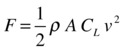
Like the drag coefficient Cd, the lift coefficient CL depends on a variety of factors. For aircraft, the important variables are wing shape and angle of attack.
As we did for the drag force, we can define a lift constant k = 1/2 ρACL, which then enables us to write the magnitude of the lift force as F = kv2.
The direction of the lift force is perpendicular to the direction of the velocity. Taking this into account, we can define a Forces.lift() function as follows:
Forces.lift = function(k,vel) {
     var force;
     var velMag = vel.length();
     if (velMag > 0) {
          force = vel.perp(k*velMag);
     }
     else {
          force = new Vector2D(0,0);
     }
     return force;
}
Example: An airplane
Let’s now demonstrate how the lift force can make an airplane fly. The file airplane.js contains the code for a basic flight demonstration. We’ll just reproduce the key parts of the code here. First, take a look at the variable declarations/initializations and the init() function:
var plane;
var m = 1;
var g = 10;
var kDrag = 0.01;
var kLift = 0.5;
var magThrust = 5;
var groundLevel = 550;
var t0,dt;

window.onload = init;

function init() {
     makeBackground();
     makePlane();
     t0 = new Date().getTime();
     animFrame();
};
The variable names should be self-explanatory. The makeBackground() and makePlane() methods produce the visual setup you can see in Figure 7-16. In makePlane(), a plane is created as an instance of the Plane object and placed on the “runway” with an initial velocity of zero. You are welcome to take a look at the plane.js file to see what the code for the Plane object looks like (or even improve on it, if you feel so inclined!). But the visual details are not important for our present purpose. What really matters is how to make the plane fly. This is initiated, as ever, by the animFrame() and related methods. The only new code here is in calcForce().
As depicted in Figure 7-15, there are four main forces on an airplane in flight: gravity (W), thrust (T), drag (D), and lift (L). When the airplane is on the ground, there is also the normal contact force due to the ground. Hence, the calcForce() method computes these forces and adds them up:
function calcForce(){
     var gravity = Forces.constantGravity(m,g);
     var velX = new Vector2D(plane.vx,0);
     var drag = Forces.drag(kDrag,velX);
     var lift = Forces.lift(kLift,velX);
     var thrust = new Vector2D(magThrust,0);
     var normal;
     if (plane.y >= groundLevel-plane.height){
          normal = gravity.multiply(-1);
     }else{
          normal = new Vector2D(0,0);
     }
     force = Forces.add([gravity, drag, lift, thrust, normal]);
}
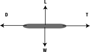
Figure 7-15. The four forces on a airplane in flight
Gravity is straightforward as usual. The drag and lift forces are computed in a simplified way, by considering only the horizontal component of the airplane’s velocity. Also, the airplane is assumed to be horizontal at all times, with an angle of attack that is zero. The thrust is modeled as a constant force. Finally, the normal force is set to be equal and opposite to gravity when the plane is on the ground, and zero otherwise.
When you run the simulation, you’ll see that the plane takes off only when it has attained a high enough velocity to create sufficient lift to overcome its weight (see Figure 7-16). If you reduce the magnitude of the thrust magThrust to 3 or 4, the plane moves along the runway, but it never takes off. Under the horizontal thrust and drag forces, it attains a maximum horizontal velocity (similar to terminal velocity) that is insufficient to generate enough lift to overcome its weight.
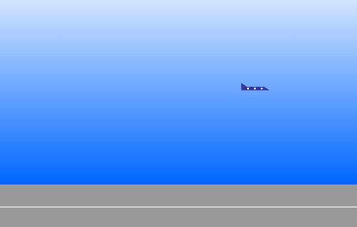
Figure 7-16. Plane flying thanks to the lift force
To reiterate, we’ve made a lot of simplifications in this example. We’ll build a much more complete and realistic flight simulator in the final chapter, in which we’ll also look at the drag, lift, and thrust forces on an airplane in more detail.
Wind is not itself a force, but it can generate forces. Wind is the movement of air, and it has an associated velocity at each point in space and time. It can be quite complicated, but fairly realistic effects can be achieved even with simple models of the wind. A constant wind blowing over a stationary object can be viewed in a similar way to an object moving through air, with the direction reversed. It generates drag and lift forces in a similar way.
Force due to the wind
As you saw at the beginning of the chapter, moving fluids have an associated dynamic pressure. Wind is nothing but moving air. When wind blows on an object or surface, it therefore exerts a force due to the dynamic pressure.
How do we calculate this force? According to what we said, only the relative velocity matters. So, the force exerted by the wind is just the drag force in reverse, where w is the wind velocity:
Hence, we can use the drag force function to model wind, using the wind velocity and a negative drag constant k.
Wind and drag
An object moving in air will, of course, still experience drag, even in the presence of wind. Therefore, the net force due to the motion of the object and that of the air (wind) will be the drag force taking as reference the relative velocity between the object and the air. Therefore, the combined force due to wind and drag is given by the following, where |w – v| denotes the magnitude of the vector (w – v):
Note that |w – v| is not usually equal to the difference (w – v) in the magnitudes of w and v.
We can use the drag force function to compute the combined effect of wind and drag by using the relative velocity between an object and the air.
Steady and turbulent flow
We now know how to calculate the force on an object in the presence of wind given the wind velocity. But how do we model the wind velocity w itself?
The answer is that it depends on the situation we are modeling. The behavior of the wind is rather complicated because it varies both in space and in time. Wind depends on complex atmospheric conditions as well as obstacles such as buildings and trees. However, for most purposes, you’d probably want to keep things as simple as you can get away with. So we’ll discuss only some simple ways of modeling the wind velocity.
The simplest model of the wind is to assume that the velocity w is constant both in space and time. This corresponds to what is called a uniform and steady flow. A slightly more complicated model is to assume a steady flow (still constant in time) that is constant horizontally but varies with height. This model would account for the fact that the wind speed is lower near the ground and becomes higher farther up.
In the real world, the wind is usually not steady but consists of gusts that blow apparently randomly. The gusts produce what is called turbulent flow, which can make things move in complex ways.
Example: Air bubbles in a steady wind
In this example, we’ll model a steady and uniform wind blowing some bubbles in air. The file bubbles-wind.js contains the code. Since it is a little different than in previous examples (because it involves multiple particles), we reproduce the code in full here:
var canvas = document.getElementById('canvas'),
var context = canvas.getContext('2d'),

var bubbles; var t0;
var dt;
var force;
var acc;
var numBubbles = 10;
var g = 10;
var rho = 1;
var rhoP = 0.99;
var kfac = 0.01;
var windvel = new Vector2D(40,0);

window.onload = init;

function init() {
     bubbles = new Array();
     var color = 'rgba(0,200,255,0.5)';
     for (var i=0; i<numBubbles; i++){
          var radius = Math.random()*20+5;
          var V = 4*Math.PI*Math.pow(radius,3)/3;
          var mass = rho*V;
          var bubble = new Ball(radius,color,mass,0,true);
          bubble.pos2D = new Vector2D(Math.random()*canvas.width,Math.random()*canvas.height);
          bubble.velo2D = new Vector2D((Math.random()-0.5)*20,0);
          bubble.draw(context);
          bubbles.push(bubble);
     }
     t0 = new Date().getTime();
     animFrame();
};

function animFrame(){
     requestAnimationFrame(animFrame,canvas);
     onTimer();
}
function onTimer(){
     var t1 = new Date().getTime();
     dt = 0.001*(t1-t0);
     t0 = t1;
     if (dt>0.2) {dt=0;};
     move();
}
function move(){
     context.clearRect(0, 0, canvas.width, canvas.height);
     for (var i=0; i<numBubbles; i++){
          var bubble = bubbles[i];
          moveObject(bubble);
          calcForce(bubble);
          updateAccel(bubble.mass);
          updateVelo(bubble);
     }
}
function moveObject(obj){
     obj.pos2D = obj.pos2D.addScaled(obj.velo2D,dt);
     obj.draw(context);
}
function updateAccel(mass){
     acc = force.multiply(1/mass);
}
function updateVelo(obj){
     obj.velo2D = obj.velo2D.addScaled(acc,dt);
}
function calcForce(particle){
     var V = particle.mass/rhoP;
     var k = Math.PI*particle.radius*particle.radius*kfac;
     var gravity = Forces.constantGravity(particle.mass,g);
     var upthrust = Forces.upthrust(rho,V,g);
     var relwind = windvel.subtract(particle.velo2D);
     var wind = Forces.drag(-k,relwind);
     force = Forces.add([gravity, upthrust, wind]);
}
In init() we’re creating a lot of bubbles as Ball objects and giving each a random radius. (If you have a slow computer, you may want to reduce the number of bubbles!) Their volume and mass are then calculated using the formula for the volume of a sphere and the density of the bubbles, which is specified as 0.99. The bubbles are given a random position and a small random horizontal velocity. Then they are collected into an array, which is then used in the move() method to apply the methods moveObject(), calcForce(), updateAccel() and updateVelo() to each bubble in turn.
In the calcForce() method, three forces are calculated and added: gravity, upthrust, and the wind (drag) force. The upthrust is calculated using the volume of each bubble, worked out using the formula volume = mass/density. To compute the force due to wind, the relative velocity relwind is computed by subtracting the bubble’s current velocity from the velocity of the wind windvel, which is given as a constant horizontal vector. The wind/drag force is then calculated by using Forces.drag() with a negative drag coefficient –k and the relative velocity as arguments. Note that k includes a factor equal to the bubble’s projected area, taking into account that the drag force is proportional to the area of an object.
If you run the simulation, you’ll see that the bubbles drift in the direction of the wind while rising slowly, as you’d expect (see Figure 7-17). Play with the wind velocity and other parameters to see how the motion is modified.
Figure 7-17. Bubbles in a steady wind
Turbulence is a complex phenomenon. In fact, it is so complex that you need huge supercomputers with hundreds of processors to compute turbulent flows accurately even for simple configurations. On the other hand, there are numerous approaches for modeling turbulence in an approximate way. One simple approach is to use random numbers.
You can produce effects that look like turbulence by superimposing random noise on an otherwise steady wind field. This exploits the statistical properties of turbulence, which can usually be represented by decomposing the wind velocity at any time in the following way, where wsteady is a steady part and wfluctuating is a time-varying part that captures the turbulent fluctuations:
![]()
The steady part wsteady is just a constant vector, as we modeled in the previous bubbles simulation. We can model wfluctuating by a vector whose components are random numbers that are updated at each timestep. To do this in the bubbles simulation, just add the following line of code in calcForce() before the line that computes relwind:
windvel = new Vector2D(20 + (Math.random()-0.5)*1000,(Math.random()-0.5)*1000);
We did this and saved the new file as bubbles-turbulence.js. We also added some code to indicate the variation of the wind vector w in a function showArrow() called from move(). The code produces a line in the middle of the stage directed along the instantaneous wind direction and with length proportional to the magnitude of the wind velocity.
The preceding line of code specifies the wind velocity w as the sum of a steady wind vector (20, 0) that blows to the right at 20 pixels per second, and a random wind vector (Math.random()-0.5)*1000,(Math.random()-0.5)*1000) with x and y components that range from –500 to 500 pixels per second. The wind velocity is the same at all locations on the stage.
Experiment by changing these values to whatever you like. The magnitude of the steady wind (here set by the value of 20) gives the bubbles a steady drift. The magnitude of the fluctuations (here set by the factor of 1000), controls the gustiness of the wind and makes the bubbles fluctuate. You can produce a fairly convincing turbulence effect in this way.
Summary
This chapter introduced a number of forces that act on solid objects in contact with other solid objects or with fluids. If you are simulating nearly anything on Earth, chances are you’ll need to model these forces. What you learned in this chapter has given you a solid foundation upon which you can build to create more complex effects and simulations. In the final chapter, you will have the opportunity to develop more complete simulations using the physics explained here. Meanwhile, in the next chapter, you will be introduced to a new type of force that produces oscillatory (spring-like) motion.