![]()
Gravity, Orbits, and Rockets
Starting in this chapter, you’ll explore many different forces and the types of motion they produce. Here we focus exclusively on the force of gravity. You’ll learn how gravity makes things move both on Earth and in space. And before you know it, you’ll be able to code up orbits and rockets!
Topics covered in this chapter include the following:
- Gravity: Gravity, or gravitation, is the force that the Earth exerts on all objects near it. But there is a lot more to gravity than we’ve discussed so far.
- Orbits: An example of the effect of gravity is to keep planets in their orbits around the Sun. Learn how to easily build simple orbit simulations.
- Local gravity: How gravity behaves at the local scale, near the surface of the Earth.
- Rockets: Build a simple rocket, launch it, and make it orbit a planet.
Gravity
As inhabitants of a planet, we are aware of gravity perhaps more than any other force. Gravity, also known as gravitation, will play a part in most of the simulations you’ll build in this book. In fact, you’ve already come across several examples. However, in all the cases you’ve met so far, we’ve dealt with gravity as it exists near the surface of the Earth—as a constant force. It’s now time to take a deeper look at gravity.
Let’s first recap briefly what you have already learned about gravity in the previous chapters. If an object has mass m, then Earth exerts a force on it that points vertically downward. The magnitude of this force of gravity is equal to mg, where g is a constant equal to approximately 9.81 m/s2 near the Earth’s surface. This force is also called the weight of the object.
The constant g is equal to the acceleration that any object would experience if it were to move under the sole effect of gravity. We can see this by using Newton’s second law, F = ma. If the resultant force F is just the force of gravity, then F = mg. Hence, we have this:
![]()
And dividing both sides by m gives us this:
![]()
This result tells us that all objects moving under the action of gravity as the only force experience the same acceleration regardless of their mass, or indeed, of any other properties. So, assuming all other forces can be neglected, if you drop a hammer and a house from the same height, both would accelerate at the same rate and therefore fall at the same time!
Of course, if you drop a feather, it will take much longer to fall. That’s because there is an upward drag force due to air that opposes its fall. There is also a drag force in the cases of a stone or a house, but in those cases that force is negligibly small compared with their weight, and so has a negligible impact on their motion. If you were to drop a feather and a hammer on the Moon, where there is no air and therefore no drag, they would both fall at the same time. In fact, the astronaut David Scott did exactly that during the Apollo 15 mission. You can even see a video of this feat on NASA’s web site or on YouTube (search for “hammer and feather”).
Newton’s universal law of gravitation
The Earth is not the only object that exerts a force of gravity. Newton taught us that any object exerts a gravitational pull on any other object. So not only does the Earth exert a gravitational force on us, but each of us also exerts a gravitational force on the Earth, and indeed on each other, too!
Newton gave an exact formula for calculating the gravitational force between any two objects, which is the force law for gravity:
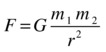
In this formula, m1 and m2 are the masses of the objects involved, and r is the distance between their centers. The symbol G is a universal constant with the value of approximately 6.67 × 10⁻¹¹ Nm2/kg2. It is called the gravitational constant. By universal, we mean that it has the same value irrespective of the properties of the interacting objects. Newton postulated that the same formula, with the same value of G, holds for any two objects—from tiny particles to planets and stars. Hence, we call it Newton’s universal law of gravitation.
Let’s try to understand what this formula is telling us. First of all, the gravitational force F is proportional to the masses m1 and m2 of the two objects. Therefore, the larger those masses are, the larger the force will be. Second, the force is inversely proportional to the square of their distance apart; that means we are dividing by r2. Therefore, the greater the distance between the two objects, the smaller the force will be (because we’ll be dividing a number by the square of a very large number). Third, because we are multiplying by a small number G (6.67 × 10⁻¹¹ is equal to 0.0000000000667), the force will be tiny except when very large masses are involved. So, gravity is a very weak force, except when at least one of the objects has a very large mass.
To give you an idea of what we mean, let’s calculate the gravitational force between two persons (whom we’ll call Joe1 and Joe2) of mass 80 kg each standing a distance of 1 m apart, and compare it with the gravitational force that the Earth exerts on each of them.
Using the previous formula, the force between Joe1 and Joe2 is given by F = 6.67 × 10-11 × 80 × 80 / 12 N = 4.3 × 10⁻⁷ N (approximately). That’s 0.43 millionth of a newton.
The force that the Earth exerts on each is, of course, equal to their weight: mg = 80 × 9.81 N = 785 N (approximately). You can also work it out using the previous formula and the mass (5.97 × 1024 kg) and radius (6.37 × 10⁶ m) of the Earth as F = 6.67 × 10-11 × 5.97 × 1024 × 80 / (6.37 × 10⁶)2 N = 785 N. That’s nearly 2 billion times larger!
We haven’t said anything about the direction of the force yet. Newton said that the force always acts along the line that joins the centers of the two objects (see Figure 6-1).
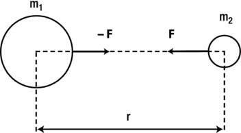
Figure 6-1. Newton’s law of universal gravitation
Also note that the forces on Joe1 and Joe2 form an action-reaction pair. So Joe1 exerts a force of 4.3 × 10⁻⁷ N on Joe2, and vice versa, with the two forces being equal and opposite—and similarly for the force between each of the two Joes and the Earth.
Creating the gravity function
We’ll now create a static method of the Forces object that will implement gravity in the form of Newton’s law of gravitation. The method will take as input the variables that go into the force law for gravity, namely G, m1, m2, and r. It must return a vector force. Therefore, we need a vector form for Newton’s law of gravitation that implements the fact that the force points along the line joining the two objects. Let’s just give the formula and explain it afterward:
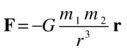
Comparing that with the previous formula for the force law for gravity, what we’ve done is write the force as a vector; then we multiplied the force magnitude by –r/r. Recall from Chapter 3 that r/r is a unit vector in the direction of r, where r here is the position vector of one of the objects relative to the location of the other object.
As shown in Figure 6-2, r is the difference in the position vectors of the two objects, and r is its magnitude, which is simply the distance between the two objects. Recall that there are two forces, not one: the force on object 1 due to object 2, and vice versa. These two forces have the same magnitude but the opposite direction. We always define r to be the position vector of the object on which the force is acting, relative to the object that is exerting the force. We need the minus sign because that force is directed in the opposite direction to r.
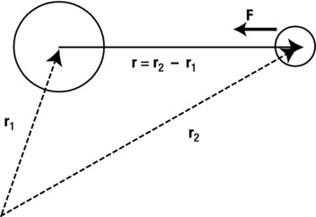
Figure 6-2. Vector form of Newton’s law of universal gravitation
Here is the static method to implement the gravity force:
Forces.gravity = function(G,m1,m2,r){
     return r.multiply(-G*m1*m2/(r.lengthSquared()*r.length()));
}
We just use the multiply() method of the Vector2D object to return a new vector that multiplies r by (-G m1m2/r3). Let’s now use this gravity() method in the next few examples.
Before we can apply the gravity function, we have to choose suitable values for G, m1, m2, and r. Remember that we are modeling motion on a computer screen. Therefore we have to scale physical values appropriately so that we get the right amount of motion on the screen in a sensible time. For example, if we were simulating the motion of the Earth around the Sun, we wouldn’t want to use the real values of all the variables, such as the mass of the Sun, and so on. Doing that would mean we’d have to wait for a year to see the Earth go once around the Sun!
In Part IV, we’ll show you how to create a scaled computer model properly. For now, we’ll simplify the approach and make some suitable choices just to make the motion look roughly right on the screen. To do this, we’ll choose our own units for all the variables of the model.
Let’s start with the distance r. That’s an easy one—the natural unit to use here is pixels. This leaves us with mass and G. We can give G any value we like, so let’s choose G = 1. Having made these two choices, we now need to choose suitable values for the masses so that the right amount of motion is produced to be noticeable on the screen. Let’s look at an example: orbits!
With our gravity function, it’s very easy to create a realistic-looking orbital simulation. Figure 6-3 shows a screenshot of what we’ll create: a planet orbiting a sun, against a background of fixed stars. For simplicity, we assume that the sun remains fixed. In reality, as we saw previously, both the sun and the planet will experience a gravitational force of the same magnitude but in opposite directions (with the force on each one pointing toward the other). So both the planet and the sun will move. But if the mass of the sun is much larger than that of the planet, the motion of the sun will be so small it will hardly be perceivable, anyway. That’s because F = maagain, so that the acceleration a = F/m. Thus, if the mass m is very large, the acceleration a will be very small. So to save coding and CPU time, we can neglect the motion of the sun altogether.

Figure 6-3. A planet orbiting a stationary sun
The orbits code
The code to achieve a basic orbit simulation is simpler than you think. The file orbits.js contains the code, shown here in its entirety:
var canvas = document.getElementById('canvas'),
var context = canvas.getContext('2d'),
var canvas_bg = document.getElementById('canvas_bg'),
var context_bg = canvas_bg.getContext('2d'),

var planet;
var sun;
var m = 1; // planet's mass
var M = 1000000; // sun's mass
var G = 1;
var t0,dt;

window.onload = init;

function init() {
     // create 100 stars randomly positioned
     for (var i=0; i<100; i++){
          var star = new Ball(Math.random()*2,'#ffff00'),
          star.pos2D= new Vector2D(Math.random()*canvas_bg.width,Math.random()*canvas_bg.height);
          star.draw(context_bg);
     }
     // create a stationary sun
     sun = new Ball(70,'#ff9900',M,0,true);
     sun.pos2D = new Vector2D(275,200);
     sun.draw(context_bg);
     // create a moving planet
     planet = new Ball(10,'#0000ff',m,0,true);
     planet.pos2D = new Vector2D(200,50);
     planet.velo2D = new Vector2D(70,-40);
     planet.draw(context);
     // make the planet orbit the sun
     t0 = new Date().getTime();
     animFrame();
};

function animFrame(){
     animId = requestAnimationFrame(animFrame,canvas);
     onTimer();
}
function onTimer(){
     var t1 = new Date().getTime();
     dt = 0.001*(t1-t0);
     t0 = t1;
     if (dt>0.1) {dt=0;};
     move();
}
function move(){
     moveObject(planet);
     calcForce();
     updateAccel();
     updateVelo(planet);
}

function moveObject(obj){
     obj.pos2D = obj.pos2D.addScaled(obj.velo2D,dt);
     context.clearRect(0, 0, canvas.width, canvas.height);
     obj.draw(context);
}
function calcForce(){
     force = Forces.gravity(G,M,m,planet.pos2D.subtract(sun.pos2D));
}
function updateAccel(){
     acc = force.multiply(1/m);
}
function updateVelo(obj){
     obj.velo2D = obj.velo2D.addScaled(acc,dt);
}
The code is very straightforward. First, we create a group of 100 stars as Ball instances and place them randomly on the stage. This is, of course, purely for aesthetic reasons. If you don’t like stars, go ahead and get rid of them. Next we create a sun as another Ball instance, setting its radius to 70 pixels and its mass to 1,000,000. We position the sun at (275, 200). By default, the velocity of the sun is zero. Then we create a planet as a Ball instance, set its radius to 10, and set its mass to 1. The initial position and velocity of the planet are then set.
The animation loop is similar to previous examples; the only difference is that we’ve chosen to pass the planet as a parameter in moveObject() and updateVelo(), just for some variety. Remember that updateAccel() implements Newton’s second law, F = ma, to make a particle move under forces specified in the calcForce() method. In the calcForce() function we specify the gravity force exerted by the sun on the planet as the only force. In the Forces.gravity() method, we pass the values of G (set to 1), the masses of the two objects, and the position vector of the planet relative to that of the sun: planet.pos2D.subtract(sun.pos2D).
Go ahead and run the code—it really works!
Observe that the planet tries to move away at its initial velocity, but is pulled back by the sun’s gravity. You might wonder why the planet does not fall into the sun. Well, in fact it is “falling” toward the sun all the time but, because of its initial position and velocity, it “misses” the sun every time. Notice also that the planet travels faster when it’s near the sun. This happens because the force of gravity is larger and therefore its acceleration is larger closer to the sun.
This code produces a realistic orbit simulation because it has basically all the physics governing orbital motion under gravity. And the physics really boils down to just four equations:

![]()


In these equations, m is the mass of the planet, and M is the mass of the sun. The first two equations are laws, and the last two are just definitions. To recap, this is what our code is doing at each timestep: From the first law, you compute the gravitational force. You then use the second law to compute the acceleration. Knowing the acceleration, you integrate the third equation to compute the velocity. Finally, knowing the velocity, you integrate the fourth equation to give the displacement. This tells you where you must move your particle at each timestep.
Try changing the parameters in the code to see their effect. For example, you can change the masses of the planet and the sun, or the initial position and velocity of the planet. We’ve chosen the mass of the sun to be 1,000,000 times that of the planet. This is a realistic ratio; for example, the mass of the Sun is 330,000 times that of the Earth and 6,100,000 times that of Mercury.
Change the mass of the sun to 2,000,000. The planet is pulled closer to the sun because the force of gravity is proportional to the mass of the sun. Doubling the sun’s mass doubles the force of gravity and therefore the acceleration toward the sun. Conversely, if you decrease the mass of the sun to 900,000, you’ll see that the sun’s pull on the planet is weaker, so that the planet wanders farther away.
Now change the mass of the planet instead. Make it 0.001 and then 1000. You’ll see that the mass of the planet has no effect on its motion. What’s going on is that you are increasing the force on the planet by increasing its mass, but then you must divide the larger force by its larger mass. Take a look at the first two equations above. In the first one, you multiply by the mass of the planet to calculate the gravitational force. In the second one, you then need to divide that force by the same mass to calculate the acceleration. The net result is that the acceleration is independent of the mass of the planet. This is just as it should be. It’s the astronomical equivalent of the hammer-and-feather experiment we mentioned at the beginning of this chapter.
Does this mean that the motion is unchanged even if the planet’s mass is comparable to that of the sun? No, not really. Remember the approximation we made at the beginning? We assumed that the mass of the sun was much larger than that of the planet, so that we could neglect the sun’s motion under the gravitational force exerted on it by the planet. If the planet’s mass is a sizeable fraction of the sun’s mass, we’ll need to model the motion of the sun too, even if we are just interested in the planet’s motion! That’s because as the sun moves around, its distance from the planet will change, which will modify the force on the planet. What we’ve done so far is to model one-body motion. To deal with this problem, we’ll need to model two-body motion. It’s not really that much more difficult, and we’ll do that later. We’ll even look at the motion of a large number of particles under mutual gravitational forces in a later chapter.
Next, experiment with different initial velocities for the planet. For example, changing the velocity vector to (70, –40) gives a more circular orbit, similar to the Earth’s orbit. A velocity of (85, –40) gives a highly elongated orbit like that of a comet. Later in the book we’ll show you how to work out the exact velocity you need to produce a circular orbit.
If the velocity of the planet is small, it will get sucked into the sun. For example, change the velocity to (0,0). The planet accelerates toward the sun’s center, as it should do, but then something weird happens when it actually gets there. For example, it might bounce back or fly off at high speed. This is an unphysical behavior, and it happens because we have not accounted for the finite size of the objects in the code. Because Newton’s law of gravitation is proportional to 1/r2, the force becomes larger as the distance r becomes smaller. For example, when r is 10 pixels, 1/r2 has the value of 0.01; when r is 1, 1/r2 is 1; and when r is 0.1, 1/r2 is 100. So when r approaches zero (when the centers of the two particles nearly coincide), the gravitational force becomes indefinitely large. At the same time, the vector r, which is the position vector pointing from the sun to the planet, becomes so small that numerical errors make its direction unpredictable. Therefore, the planet suffers a large acceleration in some apparently random direction at the center of the sun.
This is a general problem that you’ll encounter with a force law like Newton’s law of gravitation. The way you deal with it depends on precisely what you want to model. If something is falling into the sun, chances are you’d want to make it disappear when it does so—that’s simple enough to code up, and you don’t need any special physics. If something is colliding with a solid planet like the Earth, it will burn up in the Earth’s atmosphere, create a crater, or smash up the Earth, depending on its size. Any of this would be rather tricky to model in a precise way, although you could conceivably create some movie-style special effects! If something is falling into one of the gas giants like Jupiter or Saturn, you might want to model how gravity varies inside the planet. We’ll see an example of how you might be able to do that later in this chapter.
It turns out that if the velocity magnitude of a planet is less than a certain critical value, it will always be “caught” by the gravitational attraction of the sun, either orbiting or ending up in a collision with the sun. The critical value above which a planet would escape the sun’s gravity is called the escape velocity. The formula for the escape velocity is given by the following, where M is the mass of the sun and r is the distance from its center:

So the escape velocity is a function of distance from the center of the attracting body.
Note that whatever we said about a planet orbiting the sun applies more generally to any object orbiting another object under the force of gravity—for example, a satellite (natural or artificial) orbiting a planet. Hence, using the preceding formula, the escape velocity of any object at the Earth’s surface is given by the following, where Me and re are the mass and radius of the Earth, respectively:

Putting in the values for G, Me, and re into the above formula gives v = 11.2 km/s. This is the escape velocity at the Earth’s surface: if you could throw a projectile with a velocity at least equal to this velocity, it would escape the Earth’s gravity. For comparison, the escape velocity from the surface of the Sun is 618 km/s. By contrast, the escape velocity from the surface of Eros (a near-Earth asteroid with dimensions of approximately 34 km × 11 km × 11 km) is a mere 10 m/s. You could drive off the asteroid in a car!
Going back to the Orbits simulation, G = 1, the mass of the sun is 1,000,000, and the planet is initially at a distance of ![]() pixels from the sun. So the escape velocity at the initial location of the planet is
pixels from the sun. So the escape velocity at the initial location of the planet is ![]() pixels per second. You can check this with the simulation. First, change the initial velocity of the planet to (80, 0), so that its magnitude is 80. The planet will orbit the sun. Now increase the initial velocity magnitude to 100 by changing the velocity to (100, 0). The planet will move farther from the Sun but will still orbit it. Even if you change the velocity to (105, 0) and wait long enough (about five minutes or so), the planet will disappear from the edge of the canvas, but will eventually come back to complete an orbit. But if you increase the velocity magnitude beyond 109.2, it will never come back. We don’t advise you to wait!
pixels per second. You can check this with the simulation. First, change the initial velocity of the planet to (80, 0), so that its magnitude is 80. The planet will orbit the sun. Now increase the initial velocity magnitude to 100 by changing the velocity to (100, 0). The planet will move farther from the Sun but will still orbit it. Even if you change the velocity to (105, 0) and wait long enough (about five minutes or so), the planet will disappear from the edge of the canvas, but will eventually come back to complete an orbit. But if you increase the velocity magnitude beyond 109.2, it will never come back. We don’t advise you to wait!
So far, we’ve made a single object move under the gravitational attraction of another object. But we know that gravitational forces come as an action-reaction pair, so the other object must also experience an equal and opposite force. The result is that the other object will also move. It is fairly straightforward to modify the orbits.js code to implement this. The resulting code is in the file two-masses.js:
var canvas = document.getElementById('canvas'),
var context = canvas.getContext('2d'),
var canvas_bg = document.getElementById('canvas_bg'),
var context_bg = canvas_bg.getContext('2d'),

var ball1;
var ball2;
var r1 = 10;
var r2 = 40;
var m1 = 1;
var m2 = 60;
var G = 100000;
var t0, dt;

window.onload = init;

function init() {
     var ball1Init = new Ball(r1,'#9999ff',m1,0,true);
     ball1Init.pos2D = new Vector2D(150,200);
     ball1Init.draw(context_bg);

     var ball2Init = new Ball(r2,'#ff9999',m2,0,true);
     ball2Init.pos2D = new Vector2D(350,200);
     ball2Init.draw(context_bg);

     ball1 = new Ball(r1,'#0000ff',m1,0,true);
     ball1.pos2D = ball1Init.pos2D;
     ball1.velo2D = new Vector2D(0,150);
     ball1.draw(context);

     ball2 = new Ball(r2,'#ff0000',m2,0,true);
     ball2.pos2D = ball2Init.pos2D;
     ball2.velo2D = new Vector2D(0,0);
     ball2.draw(context);

     t0 = new Date().getTime();
     animFrame();
};

function animFrame(){
     animId = requestAnimationFrame(animFrame,canvas);
     onTimer();
}
function onTimer(){
     var t1 = new Date().getTime();
     dt = 0.001*(t1-t0);
     t0 = t1;
     if (dt>0.1) {dt=0;};
     move();
}
function move(){
     context.clearRect(0, 0, canvas.width, canvas.height);
     moveObject(ball1);
     moveObject(ball2);
     calcForce(ball1,ball2); // calc force on ball1 due to ball2
     update(ball1);
     calcForce(ball2,ball1); // calc force on ball2 due to ball1
     update(ball2);
}

function update(obj){
     updateAccel(obj.mass);
     updateVelo(obj);
}

function moveObject(obj){
     obj.pos2D = obj.pos2D.addScaled(obj.velo2D,dt);
     obj.draw(context);
}
function calcForce(obj1,obj2){
     force = Forces.gravity(G,obj1.mass,obj2.mass,obj1.pos2D.subtract(obj2.pos2D));
}
function updateAccel(m){
     acc = force.multiply(1/m);
}
function updateVelo(obj){
     obj.velo2D = obj.velo2D.addScaled(acc,dt);
}
What we’ve done here is basically simple. We create a couple of Ball instances, ball1 and ball2, and then make each ball move under the gravity exerted by the other. From the values specified previously, ball2 has a radius 4 times larger than ball1 and a mass 60 times larger. Also, ball1 has an initial velocity of (0, 150), whereas ball2 is initially stationary. We also create two more Ball instances, ball1Init and ball2Init, to indicate the initial positions of their respective counterparts in a lighter color.
Comparing two-masses.js with orbits.js, you’ll see that we have restructured some of the animation loop and physics code. To begin with, the calcForce() method now takes two arguments: the first argument is the ball that experiences the force; the second argument is the ball that exerts the force. The updateAccel() method now also takes an argument, the mass of the object whose acceleration is being calculated. For convenience we’ve also introduced a new function update(), which groups together calls to updateAccel() and updateVelo(). The move() method makes successive calls to moveObject(), calcForce() and update() for each ball. Note carefully the order in which these function calls are made—the order is important! We leave it as an exercise for you to figure out why and to experiment with what happens if you change the order of the function calls.
The other thing we’ve done here is to change the value of G to 100,000. You can give G any value you want if you compensate by using appropriate values for the masses to create the desired effect.
If you run the code, you’ll see that ball1 orbits ball2, while the latter appears to wobble. This makes sense. Both ball1 and ball2 experience the same force at any given time, but because ball2 is 60 times larger than ball1, its acceleration is 60 times less (applying a = F/m). Therefore, ball2 moves much less than ball1, as the screenshot in Figure 6-4 suggests. Note that the two balls experience a net slow drift vertically downward. This is due to conservation of momentum (see Chapter 5): the total initial momentum is nonzero (ball1 is initially moving vertically downward while ball2 is initially at rest), so this vertically downward momentum must be conserved at all times, even as ball2 moves. You can easily eliminate this drift by imparting to ball2 an initial velocity such that the total initial momentum of the system is zero, that is, m1 × u1 + m2 × u2 = 0. Hence, the initial vertical velocity of ball2 is u2 = –m1 × u1/m2 = –1 × 150/60 = –2.5 px/s. Implement this by adding the following line of code after ball2 is created:
ball2.velo2D = new Vector2D(0,-2.5);

Figure 6-4. Two-body motion (lighter images show initial positions of respective balls)
If you now rerun the code, you will find that the residual drift has disappeared, and that ball2 experiences only a slight wobble as a result of the gravitational force exerted by ball1.
Now make the mass and size of ball2 the same as those of ball1 by modifying the appropriate line so that it reads thus:
ball2 = new Ball(r1,'#ff0000',m1,0,true);
Then change the initial velocities of the two balls by making the following changes to the code:
ball1.velo2D = new Vector2D(0,10);
ball2.velo2D = new Vector2D(0,-10);
If you now run the code, you’ll find that the two balls orbit each other in a strange sort of dance, alternately coming together and then moving farther away. What is happening is that they are orbiting a common center, known as their center of mass. In fact, this was also happening when the balls had different masses; but the center of mass then was within the large ball, so that it appeared to wobble.
We are most familiar with gravity close up. How does local, near-Earth gravity relate to what you’ve learned so far? In this section, we establish the connection between Newton’s universal law of gravitation and the formula F = mg that we previously used for gravity. This will lead us to clarify the significance of the acceleration due to gravity g. We’ll then discuss how g varies with distance from the center of the Earth, and how it differs on other celestial bodies.
The force of gravity near the Earth’s surface
Time to come back to Earth! At the beginning of this chapter (as well as in previous chapters), we said that the force of gravity near the Earth on an object of mass m is given by F = mg, with g being approximately 9.81 m/s2. Then, for most of this chapter so far, we’ve been using Newton’s law of universal gravitation, which says that the gravitational force is given by F = Gm1m2/r2. How do we reconcile those two different formulas?
The answer is that they are both correct. If M is the mass of the Earth (or any other planet or celestial body we’re considering), and m is the mass of an object on or near it, the second formula gives this:

This has to give the same force as F = mg. Therefore, this must be true:
Now we can divide both sides of this equation by m to get rid of it. We are then left with this:

This formula shows that g is related to the mass M of the Earth and the distance r from its center. It tells us that g is actually a “nickname” for GM/r2.
If an object is sitting on the Earth’s surface, its distance from the Earth’s center is equal to the radius of the Earth. The mass of the Earth is 5.974 × 1024 kg and its radius is 6.375 × 10⁶ m.
Therefore, using the last formula, the value of g at the Earth’s surface is given by this, which is the exact value that was quoted before:
g = 6.67 × 10-11 × 5.974 × 1024 / (6.374 × 10⁶)2 = 9.81 m/s2
Therefore, F = mg is consistent with Newton’s law of universal gravitation.
Because it is always pointing toward the Earth’s center, gravity acts vertically downward wherever we are on or near the Earth’s surface (see Figure 6-5).
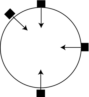
Figure 6-5. Near-Earth gravity
Variation of gravity with height
The formula g = GM/r2 tells us that we can use F = mg to calculate the force of gravity at any distance from the Earth, provided that we account for the variation of g with distance from the center of the Earth.
If an object is at a height h above the surface of the Earth, its distance from the Earth’s center is given by the following, where R is the radius of the Earth:
![]()
Therefore, the value of g at a height h above the Earth’s surface is given by this:
Because the value of g at the Earth’s surface is 9.81 m/s2, a little bit of algebra gives the two equivalent formulas:


Using this formula, you can show that the value of g at the height of the International Space Station, which is 350 km above the Earth’s surface, is about 8.8 m/s2. The value of g at the distance of the Moon (384,000 km away) is approximately 0.0026 m/s2. Remember that g gives you the acceleration of an object under gravity, and this acceleration is independent of the mass of the object. So, if the Moon were replaced with a football, it would experience the same acceleration.
You might be curious to know how g varies within the Earth. A simple model shows that g decreases approximately linearly from the surface of the Earth down to zero at the Earth’s center. The formula is as follows, where R is the radius of the Earth:
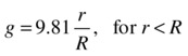
Figure 6-6 shows the variation of g with normalized distance r/R from the Earth’s center. As you can see, g increases linearly from the center of the Earth up to its surface (where r/R = 1 and g = 9.81). It then decreases rapidly with the inverse square of distance from the Earth’s center.
Figure 6-6. Variation of g with distance from the center of the Earth
Gravity on other celestial bodies
The formula g = GM/r2 allows you to calculate the value of g on other celestial bodies such as planets and stars, if you know their mass and radius.
Table 6-1 shows the approximate value of g on the surface of a few celestial bodies. These values show that the Sun’s gravity is about 28 times that of Earth, while the Moon’s is about one-sixth that of Earth. The value of g on the surface of Jupiter, the largest planet in the solar system, is about 2.5 times that of Earth. Ceres and Eros are asteroids, and their gravity is extremely weak: Earth’s gravity is about 36 times that of Ceres and more than 1660 times that of Eros.
Table 6-1. Gravity on Selected Celestial Bodies
Celestial Body |
Value of g in m/s2 |
|---|---|
Earth |
9.81 |
Sun |
274 |
Moon |
1.6 |
Jupiter |
25 |
Ceres |
0.27 |
Eros |
0.0059 |
Rockets are used for a variety of purposes, including launching spacecraft and missiles or as fireworks. In all rocket types, the rocket is propelled by exhaust formed from burning propellants within the rocket. In what follows, we give a very simplified account of the physics involved in rocket motion and show you how to put together a simple rocket simulation that can be incorporated in your games.
It is rocket science!
Without going into engineering details on the operation of various types of rocket engines, let’s just say that hot gases at high pressure are produced and pushed through a nozzle at high velocity. By Newton’s third law, the exhaust gases push back upon the rocket, propelling it forward. The forward force generated is called the thrust.
Apart from the thrust, there may be other forces on the rocket, depending on where it is and how it’s moving. Gravity is one of them. If the rocket is traveling through the Earth’s atmosphere, it will also experience a retarding drag force as well as a lift force (see the next chapter). We’ll neglect the effects of drag and lift here.
On Earth, there will also be effects due to the variation of pressure with altitude, which will affect the thrust, drag, and lift. We’ll neglect those effects, too.
As the rocket rises, the strength of the gravity that it experiences decreases in the manner described earlier in this chapter. We will account for this effect.
Rockets generally carry a substantial proportion of their mass as fuel. Therefore, the mass of a rocket will vary substantially as the fuel gets used up. This decrease in mass will affect the acceleration of the rocket and must therefore be included in the modeling.
Modeling the thrust of a rocket
To model the thrust on a rocket, we make use of the alternate form of Newton’s second law given in Chapter 5.
Remember that the force needed to move a substance at the rate of dm/dt at a velocity v is given by the formula F = vdm/dt. The exhaust gases from a rocket exit at an effective exhaust velocity ve and at a mass rate dm/dt that can be controlled. Therefore, the force on the gases is given by this:

Using Newton’s third law, the thrust on the rocket is therefore given by this:

The minus sign in the preceding vector equation means that the thrust generated is in the opposite direction to the exhaust velocity.
There may also be side thrusters on a rocket to provide a sideways thrust as needed. These work on the same principle as the main engine.
Building a rocket simulation
Okay, let’s build a rocket simulation! But before you jump up and down in glee, please note that we’ll just focus on the physics here; we leave it as an exercise for you to come up with the nice graphics and special effects.
Once again we’ll start with the orbits.js file, make some modifications, and save the new file as rocket-test.js. Here’s what it should look like:
var canvas = document.getElementById('canvas'),
var context = canvas.getContext('2d'),
var canvas_bg = document.getElementById('canvas_bg'),
var context_bg = canvas_bg.getContext('2d'),

var rocket;
var massPlanet;
var centerPlanet;
var radiusPlanetSquared;
var G = 0.1;
var dmdt = 0.5;
var dmdtSide= 0.1;
var fuelMass = 3.5;
var fuelSideMass = 3.5;
var fuelUsed = 0;
var fuelSideUsed = 0;
var ve = new Vector2D(0,200);
var veSide = new Vector2D(-100,0);
var applySideThrust = false;
var showExhaust = true;
var orientation = 1;
var animId;
var t0, dt;

window.onload = init;

function init() {
     // create 100 stars randomly positioned
     for (var i=0; i<100; i++){
          var star = new Ball(1,'#ffff00'),
          star.pos2D= new Vector2D(Math.random()*canvas_bg.width,Math.random()*canvas_bg.height);
          star.draw(context_bg);
     }
     // create a stationary planet planet
     planet = new Ball(100,'#0033ff',1000000);
     planet.pos2D = new Vector2D(400,400);
     planet.draw(context_bg);
     massPlanet = planet.mass;
     centerPlanet = planet.pos2D;
     radiusPlanetSquared = planet.radius*planet.radius;
     // create a rocket
     rocket = new Rocket(12,12,'#cccccc',10);
     rocket.pos2D = new Vector2D(400,300);
     rocket.draw(context,showExhaust);
     // set up event listeners
     window.addEventListener('keydown',startSideThrust,false);
     window.addEventListener('keyup',stopSideThrust,false);
     // launch the rocket
     t0 = new Date().getTime();
     animFrame();
};

function animFrame(){
     animId = requestAnimationFrame(animFrame,canvas);
     onTimer();
}
function onTimer(){
     var t1 = new Date().getTime();
     dt = 0.001*(t1-t0);
     t0 = t1;
     if (dt>0.1) {dt=0;};
     move();
}
function move(){
     moveObject();
     calcForce();
     updateAccel();
     updateVelo();
     updateMass();
     monitor();
}

function moveObject(){
     rocket.pos2D = rocket.pos2D.addScaled(rocket.velo2D,dt);
     context.clearRect(0, 0, canvas.width, canvas.height);
     rocket.draw(context,showExhaust);
}
function calcForce(){
     var gravity = Forces.gravity(G,massPlanet,rocket.mass,rocket.pos2D.subtract(centerPlanet));
     var thrust = new Vector2D(0,0);
     var thrustSide = new Vector2D(0,0);
     if (fuelUsed < fuelMass){
          thrust = ve.multiply(-dmdt);
     }
     if (fuelSideUsed < fuelSideMass && applySideThrust){
          thrustSide = veSide.multiply(-dmdtSide*orientation);
     }
     force = Forces.add([gravity, thrust, thrustSide]);
}
function updateAccel(){
     acc = force.multiply(1/rocket.mass);
}
function updateVelo(){
     rocket.velo2D = rocket.velo2D.addScaled(acc,dt);
}
function updateMass(){
     if (fuelUsed < fuelMass){
          fuelUsed += dmdt*dt;
          rocket.mass += -dmdt*dt;
     }
     if (fuelSideUsed < fuelSideMass && applySideThrust){
          fuelSideUsed += dmdtSide*dt;
          rocket.mass += -dmdtSide*dt;
     }
}
function monitor(){
     if (showExhaust && fuelUsed >= fuelMass){
          showExhaust = false;
     }
     if (rocket.pos2D.subtract(centerPlanet).lengthSquared() < radiusPlanetSquared){
          stop();
     }
}
function startSideThrust(evt){
     if (evt.keyCode==39){ // right arrow
          applySideThrust = true;
          orientation = 1;
     }
     if (evt.keyCode==37){ // left arrow
          applySideThrust = true;
          orientation = -1;
     }
}
function stopSideThrust(evt){
     applySideThrust = false;
}
function stop(){
     cancelAnimationFrame(animId);
}
The initial setup in init() is pretty similar to that in orbits.js, except that we now have a stationary planet in place of the sun and a rocket in place of the planet. Note that the rocket is an instance of the Rocket object, which we will look at a little later. We have introduced a couple of event listeners in init(). These listen for keydown and keyup events respectively. The corresponding event handlers startSideThrust() and stopSideThrust() set the value of a Boolean parameter applySideThrust. Whenever the right or left arrow key is pressed and held down, the applySideThrust Boolean variable is set to true; applySideThrust reverts to false when the keys are released. This variable will control the thrust applied by the side thrusters. The variable orientation is given an integer value of +1 or –1 to distinguish between right and left key presses. This variable determines the direction of the applied thrust.
In calcForce(), we specify the forces on the rocket and add them up as usual. The first force is the force of gravity that the planet exerts on it. Then there is the main thrust and side thrust. The main thrust is applied as long as there is fuel; the amount of fuel is set in the variable fuelMass. The side thrust is applied if there is fuel and if applySideThrust is true. In either case, the thrust is calculated using the formula F = –vedm/dt. The amount of fuel, exhaust velocity, and mass rate are set independently for the main thrusters and the side thrusters. (In reality, the exhaust velocity and mass rates can be varied to control the thrust, but for simplicity we’ve taken them to be fixed here.)
There are a couple of new function calls in the move() method. First, it calls a new method updateMass(). It needs to do this because the mass of the rocket is changing. The code in updateMass() checks whether there is any fuel left in the main and side thrusters; if so, it increments the mass of fuel used and decrements the mass of the rocket by the same amount. For the side thrusters, it also checks whether applySideThrust is true.
The second new function called in move() is monitor(). This method does two checks. First, it checks whether all the fuel in the main tank has been used up and, if so, it sets the value of the showExhaust Boolean variable to false, so that the exhaust will no longer be displayed at the next drawing update. The drawing of the rocket, with or without the exhaust, is done by the function call rocket.draw(context,showExhaust) in moveObject().
The second thing monitor() does is check whether the rocket collides with the planet; if so, it simply invokes the stop() method, which stops the timestepping, freezing all motion.
If you run the simulation, you’ll see that the rocket is launched automatically. It moves very slowly at first; then both its velocity and its acceleration increase until its fuel is used up. It then slows down under the gravitational pull of the planet. If you don’t do anything, it will fall back to the planet. If you press the right or left arrow keys, a side thrust will be applied to the right or left, respectively. If you apply too much or too little side thrust, the rocket will either escape the planet’s gravity or be pulled back into a collision course with the planet. See if you can make the rocket orbit the planet (Figure 6-7)! This involves applying the right amount of side thrust at the right time.
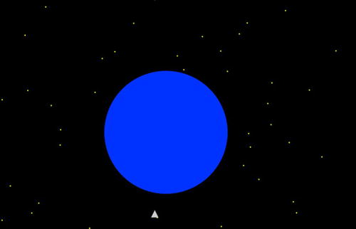
Figure 6-7. A rocket orbiting a planet!
The Rocket object
Finally, let’s take a quick look at the Rocket object that creates a visible rocket. Embarrassingly, our “rocket” is simply a triangle, with another (transparent) triangle attached at the end to represent gases from the exhaust. But please go ahead and create a better-looking version if you feel the urge to exercise your artistic skills at this point.
Here is the full source code in rocket.js:
function Rocket(width,height,color,mass){
     if(typeof(width)==='undefined') width = 20;
     if(typeof(height)==='undefined') height = 40;
     if(typeof(color)==='undefined') color = '#0000ff';
     if(typeof(mass)==='undefined') mass = 1;
     this.width = width;
     this.height = height;
     this.color = color;
     this.mass = mass;
     this.x = 0;
     this.y = 0;
     this.vx = 0;
     this.vy = 0;
}
Rocket.prototype = {
     get pos2D (){
          return new Vector2D(this.x,this.y);
     },
     set pos2D (pos){
          this.x = pos.x;
          this.y = pos.y;
     },
     get velo2D (){
          return new Vector2D(this.vx,this.vy);
     },
     set velo2D (velo){
          this.vx = velo.x;
          this.vy = velo.y;
     },
     draw: function (context,firing) {  // firing is a Boolean
          if (firing){
               var exhaust=new Triangle(this.x,this.y+0.5*this.height,this.width,this.height,'#ffff00',0.8);
               exhaust.draw(context);
          }
          var capsule = new Triangle(this.x,this.y,this.width,this.height,this.color);
          capsule.draw(context);
     }
};
Rocket draws a rocket using parameter values for width, height and color, supplied as arguments in the constructor. The code looks very similar to that for the Ball object, but with a different draw() method, which takes two parameters: context and firing. The Boolean parameter firing determines whether the ‘exhaust’ is drawn or not. Both the rocket body and the exhaust are drawn as triangles using a convenient Triangle object, which you can find in our growing objects library. Feel free to take a look at the code in triangle.js.
It’s easy to see how this simple simulation can be developed into an interesting game. Besides improved graphics and special effects, you could add extra features and controls for greater realism. With this in mind, we need to point out that there are several limitations in the way we implemented some of the operational features of the rocket. For a simple online game, these limitations probably won’t be a big deal, but they might well matter if you are trying to build a realistic simulator. In any case, it’s worth knowing about them.
We’ve already mentioned that we have fixed the thrust of the rocket in this demonstration, although in reality it can be controlled by varying the speed of exhaust and the mass rate of the ejected gases. More importantly, the directions of the main and side thrusts have been implemented in a way that is, strictly speaking, incorrect. The main thrust of a rocket acts along its axis no matter what the angle of the rocket is, and its side thrust will be at some specified angle relative to the rocket’s angle. What we did in this simplified simulation is to fix the main and side thrust to act in the vertical (y) and horizontal (x) directions, regardless of the inclination of the rocket. We also neglected the effects of air pressure, drag, and lift when the rocket is moving in an atmosphere.
Another obvious simplification we made is to put the whole rocket into orbit. In reality, space-borne rockets include one or more disposable tanks that are dropped when their fuel is used up. We leave this as an exercise for you. The Rocket class could be enhanced functionally, too. For example, it might make sense to include the amount of fuel, fuel used, exhaust velocity, and mass rate as properties of Rocket instead of hard-coding them into rocket-test.js.
Finally, the examples we coded in this chapter are realistic in that they contain the correct physics equations, but the values chosen for the various parameters are not necessarily to scale. For example, in the orbits simulation, the sizes of the planet and the sun are grossly exaggerated in comparison with their distances. This was necessary in order to see both the objects and their motion on a computer screen. Scaling issues are discussed in detail in Part IV of the book.
Summary
This chapter showed you the richness and variety that the gravitational force can exhibit, and the different types of motion it can produce. In a fairly short chapter, you’ve been able to code up orbits, two objects moving in interesting ways under their mutual gravity, and a rocket simulation from launch to orbit.
It’s amazing how much fun can be had with a just a few physics formulas and a little bit of code. You now have a taste of what can be done, even with a single force such as gravity. We’ll play more with gravity in later chapters. Meanwhile, we’ll introduce a lot of other forces in the next chapter.