![]()
Centripetal Forces: Rotational Motion
Circular and rotational motions are widespread both in nature and in man-made machines, from merry-go-rounds to the orbits and spins of planets. To analyze and model such types of motion, we need some special tools: the linear kinematics and dynamics presented in Chapter 5 need to be extended to rotational motion. In a nutshell, that is what the present chapter will begin to look into.
Topics covered in this chapter include the following:
- Kinematics of uniform circular motion: The kinematics of rotational motion can be developed in analogy with linear kinematics.
- Centripetal acceleration and centripetal force: An object in uniform circular motion still experiences acceleration and therefore a force directed toward the center of rotation.
- Non-uniform circular motion: This happens if there is a tangential component of force in addition to a centripetal component.
The material covered in this chapter will also be relevant for handling rigid body motion in Chapter 13.
Kinematics of uniform circular motion
In Chapter 4, we laid out the framework for describing motion using concepts such as displacement, velocity, and acceleration. As we said there, this framework is technically called kinematics. Those concepts sufficed to describe so-called linear or translational motion. But for analyzing circular or rotational motion, we need to introduce additional concepts.
In fact, the concepts of rotational kinematics can be developed in complete analogy with those of linear kinematics. For starters, we have rotational analogs of displacement, velocity, and acceleration that are called angular displacement, angular velocity, and angular acceleration, respectively. So let’s start by looking at them.
Recall that displacement was defined in Chapter 4 as distance moved in a specified direction. So what is the equivalent definition for angular displacement?
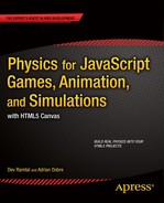
First, we need to figure out what concepts are equivalent to distance and direction in rotational motion. Take a look at Figure 9-1, which compares translational motion with rotational motion. On the left, an object moves along a distance d in a given direction. On the right, an object rotates through an angle θ about some center, in a given sense (clockwise in this case). So it’s clear that in rotational kinematics, angle takes the place of distance, and rotation sense (clockwise or counterclockwise) takes the place of direction.
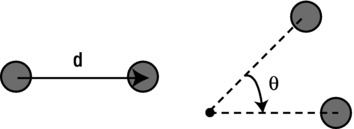
Figure 9-1. Translation and rotation compared for particle motion
Another context in which angular displacement arises is when a rigid body rotates about a fixed axis, as shown in Figure 9-2. In this case, each point on the rigid body moves through the same angle θ about the axis of rotation.
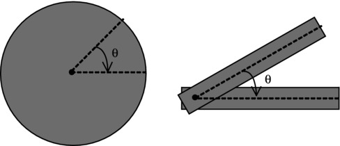
Figure 9-2. Rotation of a rigid body about an axis
In either case (particle rotation about a center or rigid body rotation about an axis), the idea is therefore the same. Hence, we define angular displacement as the angle through which an object moves about a specified center and in a specified sense.
This definition implies that the magnitude of angular displacement is an angle. The usual convention is to use radians for the angle, so we’ll do that for angular displacement.
In analogy with linear velocity, angular velocity is defined as the rate of change of angular displacement with time. The usual symbol for angular velocity is ω (the Greek letter omega), so its defining equation in calculus notation is this:

For a small time interval Δt and angle change Δθ, it can be expressed in this discrete form:

The latter equation can also be written in the following form:
![]()
This last form of the equation is what we’ll use most frequently in code to calculate the angular displacement due to an angular velocity ω in a time interval Δt.
Angular velocity is measured in radians per second (rad/s) because we divide angle by time to calculate it.
You’ll frequently deal with situations where the angular velocity is constant. For example, a particle in uniform circular motion has a constant angular velocity, although its linear velocity is not constant (because its direction of motion changes). Another example is that of an object spinning at a constant rate, such as the Earth.
Angular acceleration is the rate of change of angular velocity. It is denoted by the Greek letter α (alpha), and its defining equation is this:

The definition of angular acceleration implies that it is zero if the angular velocity is constant. Therefore, an object in uniform circular motion has zero angular acceleration. That does not mean that its linear acceleration is zero. In fact, the linear acceleration cannot be zero, because the direction of motion (and therefore the linear velocity) is constantly changing. We’ll come back to this point a little later in the chapter.
Period, frequency, and angular velocity
Uniform circular motion or rotation is a type of periodic motion (see “Basic Trigonometry” in Chapter 3) because the object returns to the same position at regular intervals. In fact, as discussed in Chapter 3, circular motion is related to oscillatory, sinusoidal motion. Back then, we defined the angular frequency, frequency, and period of an oscillation and showed that they were related by these equations:

The same relationships hold for circular motion, as should be evident by considering Figure 3-16, which illustrated them for both types of motion. For circular motion ω is now the angular velocity; it’s the same as the angular frequency of the corresponding sinusoidal oscillation. Similarly, f is the frequency of rotation (the number of revolutions per second). Finally, T is the period of revolution (the time it takes to perform one complete revolution).
As an example, let’s calculate the angular velocity of the Earth as it orbits the Sun using the formula ω = 2π/T. We know that the period T is approximately 365 days. In seconds, it has the following value:
T = 365 × 24 × 60 × 60 s ≈ 3.15 × 10⁷ s
Therefore the angular velocity has the following value:
ω = 2π/T = 2π/(3.15 × 107) ≈ 2.0 × 10⁻⁷ rad/s
This is the angle, in radians, through which the Earth moves around the Sun every second.
Let’s now calculate the angular velocity of the Earth as it revolves around its axis using the same formula. In this case, the period of revolution is 24 hours, and so T has the following value:
T = 24 × 60 × 60 s = 86400 s
Therefore, the angular velocity is the following:
ω = 2π/T = 2π/86400 = 7.3 × 10⁻⁵ rad/s
Note that this is the angular velocity of every point on the Earth, both on its surface and within it. That’s because the Earth is a rigid body so that, as it revolves about its axis, every point rotates through the same angle in the same time. However, different points have different linear velocities. How is the angular velocity related to the linear velocity? Time to find out!
The relationship between angular velocity and linear velocity
There is a simple relationship between the linear velocity and angular velocity for an object moving in uniform circular motion. To arrive at this relationship, we first note that the displacement Δs of an object moving through an angle Δθ around a circle of radius r is the length of arc that subtends that angle at the center of rotation. It is therefore given by the following:
![]()
This follows from the definition of the radian given in Chapter 3: one radian is the angle subtended at the center of a circle by an arc of length equal to the radius of the circle. So, by proportion, an arc that makes an angle of Δθ radians at the center must be of length r Δθ (see Figure 9-3).
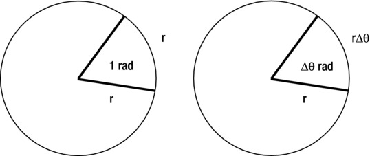
Figure 9-3. Relationship between length of arc and angle at center
Now we can divide this equation on both sides by the time interval Δt for the object to move through that angle:

But Δs/Δt = v and Δθ/Δt = ω, by definition. Hence, we have the following:
![]()
This formula gives us the linear velocity of an object moving in a circle of radius r at angular velocity ω.
It also applies to a rigid body undergoing rotation about an axis. In that case, it gives the linear velocity at a distance r from the axis of rotation. For a given angular velocity ω, the formula then tells us that the velocity is proportional to the distance from the axis (the farther away you are, the faster is the linear velocity).
Let’s apply this formula to the examples discussed in the previous section. First, we’ll calculate the linear velocity of the Earth in its orbit around the Sun. To work this out, we need to know the radius of Earth’s orbit (the distance of the Earth from the Sun): 1.5 × 10¹¹ m. We’ve already worked out the angular velocity of the Earth in its orbit. It is 2.0 × 10⁻⁷ rad/s.
Therefore, the orbital velocity of the Earth is given by the following:
v = r ω = 1.5 × 1011 × 2.0 × 10–7 = 3 × 10⁴ m/s
This is 30 km/s, or 100 000 km/hr. That’s about 100 times the typical speed of an airplane!
As a second example, because the Earth’s radius is 6.4 × 10⁶ m, and its angular velocity about its own axis is 7.3 × 10⁻⁵ rad/s (as we worked out in the previous section) the speed of any point on the Earth’s surface at the equator due to Earth’s rotation has the following value:
v = r ω = 6.4 × 106 × 7.3 × 10–5 m/s ≈ 470 m/s
This is about 1500 km/hr, or about one and a half times the typical speed of an airplane.
We now know enough to be able to put together some simple examples. Our first example will be to create rolling wheels. Unlike most of the examples in the previous few chapters, this one will not involve any dynamics, but only kinematics. So we will not compute motion using forces, but simply tell the objects how to move by specifying the velocity directly.
To begin with, let’s create a wheel. We’d like the wheel to look like that shown in Figure 9-4, with an inner and outer rim, and a number of equally spaced spokes (so that we can see it rotating).

Figure 9-4. A rolling wheel
Here is a Wheel object that does the job:
function Wheel(innerRadius,outerRadius,numSpokes){
     this.ir = innerRadius;
     this.or = outerRadius;
     this.nums = numSpokes;
     this.x = 0;
     this.y = 0;
     this.vx = 0;
     this.vy = 0;
}
Wheel.prototype = {
     get pos2D (){
          return new Vector2D(this.x,this.y);
     },
     set pos2D (pos){
          this.x = pos.x;
          this.y = pos.y;
     },
     get velo2D (){
          return new Vector2D(this.vx,this.vy);
     },
     set velo2D (velo){
          this.vx = velo.x;
          this.vy = velo.y;
     },
     draw: function (context) {
          var ir = this.ir;
          var or = this.or;
          var nums = this.nums;
          context.save();
          context.fillStyle = '#000000';
          context.beginPath();
          context.arc(this.x, this.y, or, 0, 2*Math.PI, true);
          context.closePath();
          context.fill();
          context.fillStyle = '#ffffaa';
          context.beginPath();
          context.arc(this.x, this.y, ir, 0, 2*Math.PI, true);
          context.closePath();
          context.fill();
          context.strokeStyle = '#000000';
          context.lineWidth = 4;
          context.beginPath();
          for (var n=0; n<nums; n++){
               context.moveTo(this.x,this.y);
          context.lineTo(this.x+ir*Math.cos(2*Math.PI*n/nums),this.y+ir*Math.sin(2*Math.PI*n/nums));
          }
          context.closePath();
          context.stroke();
          context.restore();
     }
}
The constructor of Wheel takes three arguments: the inner radius, the outer radius, and the number of spokes.
Now we’ll create a Wheel instance and make it roll. Take a look at the code in wheel-demo.js, from the book’s downloadable files:
var canvas = document.getElementById('canvas'),
var context = canvas.getContext('2d'),
var r = 50;       // outer radius
var w = 1;        // angular velocity in radians per second
var dt = 30/1000; // timestep = 1/FPS
var fac = 1;      // slipping/sliding factor

var wheel = new Wheel(r-10,r,12);
wheel.x = 100;
wheel.y = 200;
wheel.draw(context);

var v = fac*r*w;     // v = r w
var angle = 0;
setInterval(onTimer, 1/dt);

function onTimer(evt){
     wheel.x += v*dt;
     angle += w*dt;
     context.clearRect(0, 0, canvas.width, canvas.height);
     context.save();
     context.translate(wheel.x,wheel.y);
     context.rotate(angle);
     context.translate(-wheel.x,-wheel.y);
     wheel.draw(context);
     context.restore();
}
We create a Wheel instance and then set up a setInterval() loop that calls an onTimer() function, which increments the position and angular orientation of the wheel at each timestep. This is done using the linear velocity v and angular velocity w by using these formulas:
wheel.x += v*dt;
angle += w*dt;
The first formula uses the value of velocity v that is precalculated using this formula:
v = fac*r*w*;
This is basically the formula v = rω, but with an additional factor fac included to model the effect of slipping or sliding (skidding), with pure rolling if fac = 1.
The second formula comes from the definition of the angular velocity. The variable angle denotes the angle through which the wheel needs to be turned. The actual turning is handled by the rest of the code in onTimer(). The problem is that there is no way to rotate individual objects on a canvas element—you have to rotate the entire canvas! We do this using the context.rotate() method in the following line:
context.rotate(angle);
However, doing only this would rotate the canvas around the canvas origin (0,0), which is the top-left corner of the canvas element. We want to rotate the object around its center. To achieve this, we first use the context.translate() method to shift the canvas so that its origin is at the object’s center before the rotation. After rotating the canvas, we then translate the canvas back to its original location before drawing the wheel:
context.translate(wheel.x,wheel.y);
context.rotate(angle);
context.translate(-wheel.x,-wheel.y);
wheel.draw(context);
Note that this whole block of code is enclosed within a pair of context.save() and context.restore() commands, in order to prevent the canvas transformations from affecting other objects that may subsequently be drawn on the same canvas.
Finally, dt is the timestep, which is given a value of 0.03. This is an estimate of the time interval between successive calls of onTimer(). We expect dt to be approximately equal to 1/FPS, where FPS is the frame rate generated by the setInterval() function, which we set at 30. We reiterate that this is just approximate (refer to the discussion of setInterval() in Chapter 2), but it is good enough for this simple demo.
Run the code with fac = 1, and you’ll see the wheel move so that its translational velocity is consistent with its rotation rate. This gives the appearance of pure rolling without slipping or skidding. If you change the value of fac to less than 1, say 0.2, the wheel does not move forward fast enough in relation to its rotation; it looks like it’s stuck in the mud and is slipping. If you give fac a value greater than 1, say 5, the wheel moves forward faster than it would do purely as a result of its rotation: it appears to be skidding on ice.
Example: Satellite around a rotating Earth
What we want to achieve in this example is in essence quite simple: an animation of a satellite in a circular orbit around a rotating Earth. The twist is that we want the satellite to orbit so that it is always over the same spot on Earth. This is called a geostationary orbit; as you might guess, it’s very useful for telecommunications as well as spying.
Once again, this example will involve only kinematics and no dynamics (no forces). Later on in the chapter, we’ll add in the forces.
The full code is in the file satellite-demo.js and is reproduced here:
var canvas = document.getElementById('canvas'),
var context = canvas.getContext('2d'),

var earth;
var satellite;

var r, x0, y0, omega;
var angle = 0;

window.onload = init;

function init() {
     // create a stationary earth
     earth = new Ball(70,'#0099ff',1000000,0,true,true);
     earth.pos2D = new Vector2D(400,300);
     earth.angVelo = 0.4;
     earth.draw(context);
     // create a moving satellite
     satellite = new Satellite(8,'#0000ff',1);
     satellite.pos2D = new Vector2D(600,300);
     satellite.angVelo = earth.angVelo;
     satellite.draw(context);
     // set params
     r = satellite.pos2D.subtract(earth.pos2D).length();
     omega = earth.angVelo;
     x0 = earth.x;
     y0 = earth.y;
     // make the satellite orbit the earth
     t0 = new Date().getTime();
     t = 0;
     animFrame();
};
function animFrame(){
     animId = requestAnimationFrame(animFrame,canvas);
     onTimer();
}
function onTimer(){
     var t1 = new Date().getTime();
     dt = 0.001*(t1-t0);
     t0 = t1;
     if (dt>0.2) {dt=0;};
     t += dt;
     move();
}
function move(){
     satellite.pos2D = new Vector2D(r*Math.cos(omega*t)+x0,r*Math.sin(omega*t)+y0);
     angle += omega*dt;
     context.clearRect(0, 0, canvas.width, canvas.height);
     rotateObject(earth);
     rotateObject(satellite);
}
function rotateObject(obj){
     context.save();
     context.translate(obj.x,obj.y);
     context.rotate(angle);
     context.translate(-obj.x,-obj.y);
     obj.draw(context);
     context.restore();
}
Most of the code is straightforward, but with some noteworthy new features. We create an Earth and a satellite object. The masses that are given to these objects are irrelevant here as there is no dynamics. You can use any value you want, and the animation will behave in exactly the same way. Note that Earth is an instance of Ball, whereas satellite is an instance of Satellite. The latter object is basically like Ball, with the addition of code that draws three lines on the satellite to give it a nice old-fashioned, Sputnik-like appearance. Both the Ball and Satellite objects have a new property called angVelo, which stores the value of the angular velocity of their instances. We have also introduced an optional Boolean parameter line in Ball that, if set to true, draws a pair of crossed lines on the Ball instance. This is so that the rotation of the ball can be observed.
We give the Earth a non-zero angular velocity. Then we assign the same angular velocity to the satellite. The distance of the satellite from the Earth is computed and stored in the variable r. This distance does not change because the orbit will be circular. Then the angular velocity and x and y position of the Earth are stored in the variables omega, x0, and y0, respectively.
The action takes place in the move() method. All we are doing here is telling the satellite where it must be at any time, using these formulas:
![]()
![]()
You might recall from Chapter 3 that using cos and sin in this way produces circular motion with angular frequency ω at a radius r. Adding x0 and y0 (the coordinates of the center of the Earth) makes the satellite orbit the Earth. The other important thing is that ω is chosen to be equal to the angular velocity of the Earth. This makes the satellite orbit the Earth at exactly the same rate as the Earth spins on its axis. Run the simulation, and you’ll see that this is indeed the case.
Also, because the satellite has the same angular velocity around its axis as the Earth, its antennae always point toward the Earth (see Figure 9-5).
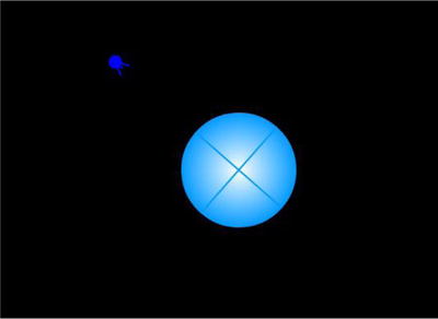
Figure 9-5. A spy satellite orbiting the Earth
The code that produces the rotation of the Earth and the satellite is in the rotateObject() method and should look familiar from the previous example. Note that here a single variable angle is used to compute the angle through which both objects must rotate at each time step. This is because they have the same angular velocity.
The alert reader will have noticed that we’ve called this example an animation rather than a simulation. That’s because we basically told the satellite how to move, rather than prescribing the forces that act on it and letting them determine the motion of the satellite. Although the animation does have some physics realism, it is not completely realistic. One reason is that we have forced the satellite to orbit the Earth at the same rate (the same angular velocity) as the Earth spins around its axis. You can change the distance of the satellite from the Earth’s center and it will still orbit at the same rate. In reality, satellites can only do so at a specific distance from the Earth’s center; in other words, all geostationary satellites must be at the same distance from the Earth! It is not obvious why that should be so, but the next section will help clarify that and help you to build this feature into the animation.
Centripetal acceleration and centripetal force
Now that we’ve covered the basics, it’s time to move on to some slightly more difficult concepts: centripetal acceleration and centripetal force. Actually they are not really difficult, but they are frequently misunderstood. Hence, we’ll try to clear up some of the possible confusion as we go along.
As we pointed out in the section on angular velocity, an object moving in a circle (or in a curved path in general) has a linear velocity that is changing with time because its direction is changing all the time. Therefore, from the definition of acceleration as rate of change of velocity, that means it has a non-zero acceleration—we never said that acceleration means just a change in the magnitude of velocity (speed); it could mean a change in direction as well.
It may not be obvious at all, but for an object moving in a circle, this acceleration actually points toward the center of the circle. Therefore, it is called centripetal acceleration (from the Latin: centr = “center,” and petere = “to seek”). One way to appreciate this is to think of the center as pulling the object, thereby changing its direction constantly (see Figure 9-6). We’ll see in a moment how to calculate the centripetal acceleration.
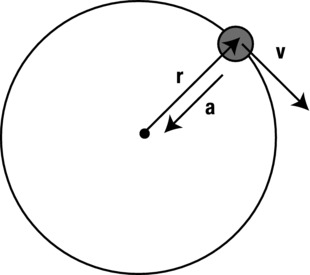
Figure 9-6. Centripetal acceleration
Centripetal acceleration must not be confused with angular acceleration. As explained earlier in this chapter, angular acceleration refers to the rate of change of angular velocity. In the case of uniform circular motion, the angular acceleration is zero because the angular velocity is constant (that’s what “uniform” means), but the centripetal acceleration is not zero. The centripetal acceleration is a measure of the rate of change of linear velocity, when the latter is only changing in direction while its magnitude remains constant.
Centripetal acceleration, velocity, and angular velocity
How do we calculate the centripetal acceleration? Well, there is a simple formula for it. It’s not easy to prove, so the best thing is just to believe us! Here is one form of the formula:

Referring to Figure 9-6, this formula tells us the centripetal acceleration for an object moving with velocity v in a circle or arc of radius r. From this we deduce that if the velocity is large, the acceleration is large (for the same radius); and if the radius is small, the acceleration is large (for the same velocity magnitude).
Remembering that v = rω, you can replace v in the preceding formula to come up with an alternative form for the formula in terms of r and ω:
![]()
This formula now tells us that the centripetal acceleration is greater when the angular velocity is greater (for the same radius). But it also tells us that the centripetal acceleration is greater when the radius is greater, for the same angular velocity. This does not contradict what we said previously about the other form of the formula, but can seem confusing at first! The key point is that here the linear velocity magnitude is not assumed to be constant for different radii. In fact, if the angular velocity is constant, then the linear velocity magnitude must increase with radius because v = rω.
One consequence of the previous formula is that for a rigid body spinning about its axis, points farther away from the axis have a greater acceleration (because all points on the rigid body have the same angular velocity) as well as a greater velocity (because v = rω).
Centripetal force
We’ve just seen that any object in uniform circular motion must experience an acceleration toward the center of the circular trajectory. Therefore, by Newton’s second law, there must be a resultant force on it that is also directed toward the center. This is known as the centripetal force.
The centripetal force is the force that is needed to keep an object in circular motion. It needs to be provided continuously by some physical agent; otherwise, the object cannot maintain circular motion.
As an example, an object whirled around by a string gets its centripetal force from the tension in the string. A car moving around a circular track gets centripetal force from friction exerted by the ground on the tires. Planets orbiting the Sun experience a centripetal force due to the Sun’s gravitational attraction.
It’s very easy to work out the formula for centripetal force. Because F = ma, you just need to multiply the formulas for centripetal acceleration by m (the mass of the moving object) to obtain this:

And to get this:
![]()
In vector form, the first formula can be written as follows:
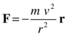
Or it can be written like this, where ru is a unit vector in the direction of the position vector r of the moving object with respect to the center:
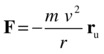
The minus sign arises because the force points toward the center (opposite to the vector r). Similar vector forms also hold for the formula F = mrω2.
Common misconceptions about centripetal force
Centripetal force is probably one of the most misunderstood concepts in physics. Let’s clear up some of the confusion.
- Centripetal force is not a distinct “type” of force in the same sense that gravity and friction are types of forces. It is simply the force that must be present to make an object move in a circle. Different forces can act as centripetal forces, including gravity and friction.
- Sometimes people mistakenly talk about the need to “balance” the centripetal force. For example, a common misunderstanding is that the gravitational force on a planet in orbit around the Sun balances the centripetal force. That does not make sense for several reasons. First, the centripetal force must point toward the Sun, and so does the gravitational force, so they are both in the same direction. Second, if the two forces did balance, the resultant force on the planet would be zero; its acceleration would therefore be zero and so it would have to move in a straight line at constant velocity (by Newton’s first law of motion). Third, centripetal force is not even a “type” of force. The correct thinking is that the gravitational force provides the centripetal force necessary for the planet to orbit the Sun.
- You may also hear about something called centrifugal force, which has the same magnitude as the centripetal force but acts in the opposite direction (away from the center of rotation). Centrifugal force is not a real force but a so-called pseudo force. It arises out of the attempt to analyze motion within the framework of Newton’s laws but from the point of view of a rotating frame of reference. An example is the description of atmospheric motion from a reference frame on the Earth (which is, of course, rotating). Although centrifugal force certainly has its place in physics in analyzing problems like this, it can cause a lot of confusion, too. Our recommendation is therefore to avoid thinking in terms of centrifugal forces. In the section ”Example: Car moving around a bend” later in the chapter we give a centripetal-force account of an example commonly thought of in terms of centrifugal force.
Example: Revisiting the satellite animation
As a first example of the application of the centripetal force concept, let’s go back to the satellite animation and inject some more realism into it as promised.
Here the centripetal force is provided by the force of gravity on the satellite. Therefore we can equate the expression for centripetal force with that for the gravitational force to obtain the following equation, where m is the satellite mass, M is the Earth mass, r is the distance of the satellite from the Earth’s center, and ω is the angular velocity of the satellite:
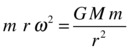
It is easy to rearrange this equation to give the following:

This formula tells us the radius at which the satellite must be in order to orbit at an angular velocity ω. In other words, the satellite cannot have just any angular velocity at any distance; the centripetal force dictates that it has to rotate at a fixed angular velocity for any given distance from the Earth! In particular, we can use the formula to calculate the distance at which it must be to rotate at the same angular velocity as the Earth’s spin. If you substitute the values for G, M (the mass of the Earth), and ω (the Earth’s angular velocity as we worked out before), you’ll find that the radius of a geostationary orbit is 42,400 km, or approximately 6.6 times the radius of the Earth.
Going back to our animation, we need to make the satellite aware of the constraint between its distance from the Earth and its angular velocity around the Earth, as expressed by the previous equation. In fact, in the animation we’ll specify the position of the satellite, and therefore the distance r from the Earth, and want to work out its resulting angular velocity ω instead of setting it to be equal to that of the Earth.
Therefore, we want a formula for ω in terms of r. It’s easy enough to manipulate the previous equation to give the following:

That’s all we need. We copied satellite-demo.js to create satellite-demo2.js. If you look at the latter file, you’ll see that the main change we’ve made is to replace this line:
omega = earth.angVelo;
with the following line:
omega = Math.sqrt(G*M/(r*r*r));
where M is the mass of the Earth (here set at 1000000), and the value of the gravitational constant G is set to 1. We now also have separate variables omegaE and angleE to store the angular velocity and angular displacement of the Earth.
If you now run the code with the previous positions and masses of the satellite and Earth and angular velocity of the Earth, you’ll see that the satellite is no longer in a geostationary orbit. In fact, by the time it completes one orbit, its antennae are already pointing the wrong way. If you use the previous formula to calculate the value of r for a geostationary orbit with the given values of G = 1, M = 1000000, and ω = 0.4, you will get r = 184.2. This is the distance that the satellite should be from the Earth’s center. Given that the Earth is located at (400,300), you just need to change the position of the satellite to a location 184.2 units away, such as (584.2,300) in satellite-demo2.js:
satellite.pos2D = new Vector2D(584.2,300);
Do this and then run the code. You’ll see that the satellite does orbit at the same angular velocity as the Earth.
Example: Circular orbits with gravitational force
In this example, we go back to a full dynamic simulation. In fact, we already did that in the orbits simulation in Chapter 6, in which we simulated the motion of a planet round the Sun. The simulation already “knows” that gravity is a centripetal force, so there is nothing else to add. But if we want circular orbits, we can use the centripetal force formula to work out exactly what velocity we need to give the planet.
Again, this is simply a matter of equating the expressions for centripetal force and gravitational force. This time, we use the form F = mv2/r for the centripetal force:
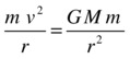
A little algebra then gives us the following, which is the velocity magnitude that the planet must have in order to have a circular orbit around the Sun at a distance r from its center:

Let’s code this into a modified version of the orbits simulation. The new source file is called circular-orbits.js, and the code is shown in full here:
var canvas = document.getElementById('canvas'),
var context = canvas.getContext('2d'),
var canvas_bg = document.getElementById('canvas_bg'),
var context_bg = canvas_bg.getContext('2d'),

var planet;
var sun;
var m = 1;       // planet's mass
var M = 1000000; // sun's mass
var G = 1;
var t0,dt;
var acc, force;

window.onload = init;
function init() {
     // create a stationary sun
     sun = new Ball(70,'#ff9900',M,0,true);
     sun.pos2D = new Vector2D(400,300);
     sun.draw(context_bg);
     // create a moving planet
     planet = new Ball(10,'#0000ff',m);
     planet.pos2D = new Vector2D(400,50);
     var r = planet.pos2D.subtract(sun.pos2D).length();
     var v = Math.sqrt(G*M*m/r);
     planet.velo2D = new Vector2D(v,0);
     planet.draw(context);
     // make the planet orbit the sun
     t0 = new Date().getTime();
     animFrame();
};

function animFrame(){
     animId = requestAnimationFrame(animFrame,canvas);
     onTimer();
}
function onTimer(){
     var t1 = new Date().getTime();
     dt = 0.001*(t1-t0);
     t0 = t1;
     if (dt>0.2) {dt=0;};
     move();
}
function move(){
     moveObject(planet);
     calcForce();
     updateAccel();
     updateVelo(planet);
}
function moveObject(obj){
     obj.pos2D = obj.pos2D.addScaled(obj.velo2D,dt);
     context.clearRect(0, 0, canvas.width, canvas.height);
     obj.draw(context);
}
function calcForce(){
     force = Forces.gravity(G,M,m,planet.pos2D.subtract(sun.pos2D));
}
function updateAccel(){
     acc = force.multiply(1/m);
}
function updateVelo(obj){
     obj.velo2D = obj.velo2D.addScaled(acc,dt);
}
Most of the code should be very familiar. The new feature in this simulation is that we give the planet exactly the initial velocity it needs to move in a circular orbit. This is done in the two lines highlighted in bold, using the formula ![]() that we just derived.
that we just derived.
Run the simulation with the initial values as given in the previous code listing, and you’ll find that the planet indeed describes a circular orbit around the Sun. To convince yourself that this works at any distance from the Sun, change the initial position of the planet to the following:
planet.pos2D = new Vector2D(400,150);
This positions the planet closer to the Sun. If you now run the code, you’ll see that the planet orbits the Sun at a faster rate, but the orbit is still circular.
Note that the velocity must be tangential with no radial component (see Figure 9-7). If there is any radial velocity component, the planet will either approach or recede from the Sun (its orbit won’t be circular). For example, with the initial position of the planet at (400, 50), try the following:
planet.velo2D = new Vector2D(v/Math.sqrt(2), v/Math.sqrt(2));
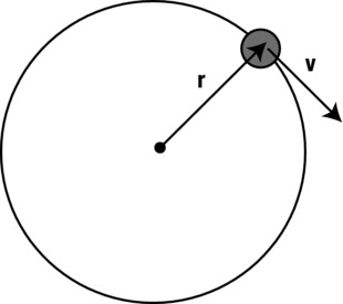
Figure 9-7. Tangential velocity
This gives the planet an initial velocity of the same magnitude v as before, but in a different direction, so that it has a radial component toward the Sun as well as a tangential component. You will find that the planet’s orbit is now highly elliptical, with the planet getting very close to the Sun and then receding away from it.
You are encouraged to try different initial positions and velocities to see the types of orbits you get. You should find that, without using the formula ![]() , it is rather hard to get the initial conditions just right to produce even approximately circular orbits by simple trial and error!
, it is rather hard to get the initial conditions just right to produce even approximately circular orbits by simple trial and error!
Example: Car moving around a bend
In the next example, we simulate the motion of a car around a circular track and use it to demonstrate skidding if the car goes too fast.
The basic physics here is that when a car moves around a curve or bend, the centripetal force it needs to do so is provided by the frictional force on the tires in contact with the road surface (see Figure 9-8).
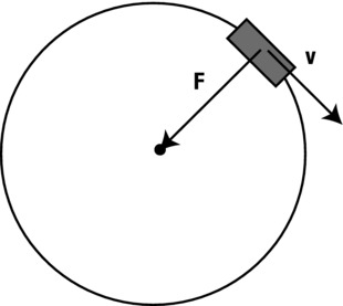
Figure 9-8. Friction provides the centripetal force for a car to negotiate a bend
Going back to the formula for centripetal force, the faster the car moves, the greater the centripetal force needed to keep it moving around the bend:

Incidentally, the formula also shows that the centripetal force is greater for sharper bends, which curve with a smaller radius.
The frictional force is the static frictional force and, as discussed in Chapter 7, it has a maximum value given by f = CsN, where N is the normal force (which here is equal to the car’s weight mg), and Cs is the coefficient of static friction between the tires and the road surface. Therefore, if the centripetal force needed to negotiate a bend exceeds the maximum static friction, the car won’t be able to follow the curvature of the bend—it will skid.
We now build a simulation that can handle this scenario in a natural way. The setup is shown in Figure 9-9.
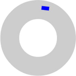
Figure 9-9. The skidding car simulation
And here is the code that does it (in the file car-demo.js):
var canvas = document.getElementById('canvas'),
var context = canvas.getContext('2d'),
var canvas_bg = document.getElementById('canvas_bg'),
var context_bg = canvas_bg.getContext('2d'),
var center = new Vector2D(canvas.width/2,canvas.height/2);
var car;
var mass = 90; // car mass
var g = 10;
var Cs = 1;
var angle = 0;
var omega;
var t0,dt;
var acc, force;
window.onload = init;
function init() {
     // create a circular track, e.g. a roundabout
     context_bg.fillStyle = '#cccccc';
     context_bg.beginPath();
     context_bg.arc(canvas.width/2, canvas.height/2, 100, 0, 2*Math.PI, true);
     context_bg.closePath();
     context_bg.fill();
     context_bg.fillStyle = '#ffffff';
     context_bg.beginPath();
     context_bg.arc(canvas.width/2, canvas.height/2, 50, 0, 2*Math.PI, true);
     context_bg.closePath();
     context_bg.fill();
     // create a car
     car = new Box(10,20,'#0000ff',mass);
     car.pos2D = new Vector2D(center.x+75,center.y);
     car.velo2D = new Vector2D(0,-10);
     car.angVelo = -car.velo2D.length()/(car.pos2D.subtract(center).length());
     omega = car.angVelo;
     car.draw(context);
     // make the car move
     t0 = new Date().getTime();
     animFrame();
};
function animFrame(){
     animId = requestAnimationFrame(animFrame,canvas);
     onTimer();
}
function onTimer(){
     var t1 = new Date().getTime();
     dt = 0.001*(t1-t0);
     t0 = t1;
     if (dt>0.2) {dt=0;};
     move();
}
function move(){
     moveObject(car);
     calcForce();
     updateAccel();
     updateVelo(car);
}
function moveObject(obj){
     obj.pos2D = obj.pos2D.addScaled(obj.velo2D,dt);
     angle += omega*dt;
     context.clearRect(0, 0, canvas.width, canvas.height);
     rotateObject(obj);
}
function rotateObject(obj){
     context.save();
     context.translate(obj.x,obj.y);
     context.rotate(angle);
     context.translate(-obj.x,-obj.y);
     obj.draw(context);
     context.restore();
}
function calcForce(){
     var dist = car.pos2D.subtract(center);
     var velo = car.velo2D.length();
     var centripetalForce = dist.unit().multiply(-mass*velo*velo/dist.length());
     var radialFriction = dist.unit().multiply(-Cs*mass*g);
     if(radialFriction.length() > centripetalForce.length()) {
          force = centripetalForce;
     }
     else{
          force = radialFriction;
     }
}
function updateAccel(){
     acc = force.multiply(1/mass);
}
function updateVelo(obj){
     obj.velo2D = obj.velo2D.addScaled(acc,dt);
}
As shown in the figure, we begin in the init() method by drawing a circular track. The next step introduces a bit of artistic novelty. Because we are dealing with a car, a Ball instance simply won’t do. Instead, our car is a Box instance. Box is a class that is essentially similar to Ball except that it draws a filled rectangle instead of a filled circle. Box takes four parameters (width, height, color, and mass), all of which have default values and are therefore optional. After creating the car as a Box instance, we position it on the track and give it an initial tangential velocity. The next line then gives the car a spin angular velocity equal to its “orbital” angular velocity by using the formula ω = v/r, where v is the car’s speed, and r is its distance from the center.
The rest of the code should be easy to follow. In calcForce(), we calculate the centripetal force using the formula F = mv2/r in vector form and the maximum frictional force on the car using the formula F = Csmg (see Chapter 7), where m is the mass of the car. For simplicity, we assume that static and dynamic friction are the same. Also, we assume that the resultant force on the car is friction in the radial direction. The if block checks whether the maximum friction is sufficient to provide the centripetal force. If so, the resultant force is taken to be equal to the centripetal force; if not, the resultant force is equal to the maximum friction.
If you run the simulation with an initial velocity of 10 or 20 px/s, you’ll find that the car moves around the track without problem. However, if you increase the velocity beyond about 30, the car will skid!
So far in this chapter we’ve dealt only with uniform circular motion. How do we handle rotation when the angular velocity is not constant? In this last section, we’ll begin to look at this problem and illustrate it with an example. A fuller treatment of non-uniform rotation will involve delving into concepts such as angular momentum and torque. For that, you’ll have to await Chapter 13.
Tangential force and acceleration
The underlying difference between uniform and non-uniform circular motion is that in the former, centripetal force is the only force; whereas in the latter there is a tangential as well as a centripetal force (see Figure 9-10). Tangential literally means “along a tangent” to the circle. The centripetal force in non-uniform circular motion is given by the same formulas as for the uniform case. As with centripetal force, the tangential force can be due to any number of factors such as gravity or friction.

Figure 9-10. Tangential (Ft ) and centripetal (Fc ) forces
Note that centripetal force changes only the direction of motion, which is why uniform circular motion is uniform. But because tangential forces act in the direction of the velocity vector, they cause a change in the speed of the rotating object. This also means there is a non-zero angular acceleration when a tangential force is present.
The bottom line: to simulate non-uniform circular motion, we need forces that will provide both centripetal and tangential force components, as demonstrated in our next and final example.
A so-called simple pendulum consists of a heavy bob suspended by a cord to a fixed pivot. The pendulum is set into oscillation by displacing the bob slightly and releasing it. Simulating a simple pendulum is not totally straightforward and does require a bit of thinking to get the physics right.
Figure 9-11 shows the force diagram for a simple pendulum. The cord will usually be inclined at some angle θ to the vertical. We assume that the cord has negligible mass and that there is no friction or drag. Let m denote the mass of the bob. There are then two forces acting on the bob: gravity acting vertically downward with magnitude mg; and the tension in the cord acting toward the fixed pivot with magnitude T.
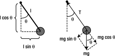
Figure 9-11. Geometrical and force diagram for a pendulum
Obviously, the bob moves in a circular arc with the pivot as its center. But the angular velocity of the bob is non-uniform. In fact, it is zero when the bob is in its uppermost position and maximum when the bob is at its lowest point. Therefore, there is an angular acceleration because of a tangential force component. Because the tension is in the radial direction (which is perpendicular to the tangential direction), it has no tangential component. But the force of gravity in general does have a tangential component given by mg sin(θ). This is the force that causes the angular acceleration. Note that because the angle θ changes with time, the tangential force and therefore the angular acceleration are not constant.
What is the radial force component that provides the centripetal force? From Figure 9-11, it’s clear that gravity has a component mg cos(θ) that acts away from the pivot. Hence, the net radial force component is T – mg cos(θ), and this must be equal to the centripetal force:
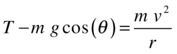
Therefore, this implies that the magnitude of the tension T is given by the following:

As is clear from Figure 9-11, the direction of the tension force is opposite to the position vector r of the bob relative to the pivot.
Now comes the clever part. All we need to do is to specify the forces of gravity mg and tension T, as given by the last equation. Then, once we give it an initial position, the bob ought to know how to move under those two forces. Let’s go ahead and code it up.
The code is in the file pendulum.js:
var canvas = document.getElementById('canvas'),
var context = canvas.getContext('2d'),

var bob;
var pivot;
var displ = new Vector2D(0,0);
var center = new Vector2D(0.5*canvas.width,50);
var mass = 1;
var g = 100;
var lengthP = 200;
var initAngle = 30;
var t0, t, dt;
var acc, force;
var animId;

window.onload = init;
function init() {
     // create a pivot
     pivot = new Ball(2,'#000000'),
     pivot.pos2D = center;
     pivot.draw(context);
     // create a bob
     bob = new Ball(10,'#333333',mass);
     bob.mass = mass;
     var relativePos = new Vector2D(lengthP*Math.sin(initAngle*Math.PI/180),lengthP*Math.cos(initAngle*Math.PI/180));
     bob.pos2D = pivot.pos2D.add(relativePos);
     bob.draw(context);
     // make the bob move
     t0 = new Date().getTime();
     t = 0;
     animFrame();
};
function animFrame(){
     animId = requestAnimationFrame(animFrame,canvas);
     onTimer();
}
function onTimer(){
     var t1 = new Date().getTime();
     dt = 0.001*(t1-t0);
     t0 = t1;
     if (dt>0.2) {dt=0;};
     t += dt;
     move();
}
function move(){
     context.clearRect(0, 0, canvas.width, canvas.height);
     drawSpring(bob);
     moveObject(bob);
     calcForce(bob);
     updateAccel();
     updateVelo(bob);
}
function drawSpring(obj){
     pivot.draw(context);
     context.save();
     context.strokeStyle = '#999999';
     context.lineWidth = 2;
     context.moveTo(center.x,center.y);
     context.lineTo(obj.x,obj.y);
     context.stroke();
     context.restore();
}
function moveObject(obj){
     obj.pos2D = obj.pos2D.addScaled(obj.velo2D,dt);
     obj.draw(context);
}
function calcForce(obj){
     displ = obj.pos2D.subtract(center);
     var gravity = Forces.constantGravity(mass,g);
     var tension;
     if (displ.length() >= lengthP) {
          tension = displ.unit().multiply(-(gravity.projection(displ)+mass*bob.velo2D.lengthSquared()/lengthP));
     }else{
          tension = new Vector2D(0,0);
     }
     force = Forces.add([gravity, tension]);
}
function updateAccel(){
     acc = force.multiply(1/mass);
}
function updateVelo(obj){
     obj.velo2D = obj.velo2D.addScaled(acc,dt);
}
We begin by creating a pivot and a pendulum bob. The bob is positioned so that the cord makes an initial angle of 30 degrees with the vertical. To see this, refer to Figure 9-11, which shows that the x and y coordinates of the bob relative to the pivot are given by the following, where l is the “length” of the pendulum, defined as the distance of the center of the bob to the fixed pivot:
![]()
![]()
Physically, l is equal to the sum of the length of the cord and the radius of the bob. In the code, we denote this by the variable lengthP. This relative position vector is calculated and stored in the variable relativePos, which is then added to the pivot’s pos2D property to set the position of the bob. The initial inclination angle (in degrees) is set by the parameter initAngle.
The novelty in the animation part of the code is basically what’s in the calcForce() method. We calculate gravity in the usual way. The if block of code checks to see if the distance of the bob from the pivot is greater than or equal to the cord length. If so, that means the cord is taut and therefore the tension is non-zero; it is calculated using the formula T = mg cos(θ) + mv2/r. Otherwise, the cord is not taut, so the tension is zero. In the current setup, it is not strictly necessary to check whether the cord is taut, because the simulation starts with a taut cord and it remains so all the time. But implementing this check makes the code more robust to possible future modifications. Note that the radial component of gravity mg cos(θ) is computed using the nifty projection() method, which we introduced into the Vector2D object so that vec1.projection(vec2) gives the projection of vector vec1 in the direction of vector vec2. Here is the definition of projection():
function projection(vec){
     var length = this.length();
     var lengthVec = vec.length();
     var proj;
     if( (length == 0) || ( lengthVec == 0) ){
          proj = 0;
     }else {
          proj = (this.x*vec.x + this.y*vec.y)/lengthVec;
     }
     return proj;
}
If you run the code and play with the parameters, you’ll see that the pendulum oscillates faster if the cord length is shorter and if the value of g is greater. This is just as it should be in reality. In fact you can test how good your simulated pendulum is by comparing the period of the oscillations with the theoretical value.
Physics theory says that for oscillations of small amplitude, the period of a simple pendulum is given approximately by the following, where l is the length of the pendulum:

The values we used in the simulation are l = 200 and g = 100. This gives you T = 2π, which is approximately 8.9 seconds. Check whether the simulation gives this value, by outputting the time to the console and timing to ten oscillations, for example, and then dividing the total time by ten. To make this easier, the file pendulum2.js includes some additional code to allow you to stop the simulation by clicking the mouse. You should get a value very close to 8.9 s. As you can see in Figure 9-12, it works almost like the real thing!.
Figure 9-12. The pendulum simulation
Summary
This chapter introduced some of the physics needed to handle circular and rotational motion, focusing on particle and simple rigid body rotation. This chapter has laid the foundations for a more detailed look at rigid body rotation, which we’ll present in Chapter 13. Some of the concepts introduced here will also be applied and developed further in the next chapter, on long-range forces.