![]()
Extended Objects
In much of this book, we have focused on the motion of particles. In this chapter, we will explore the physics governing the motion of extended objects. This topic is important for obvious reasons: objects in everyday life are extended in space and have all sorts of shapes, sizes and behavior. To model the motion of extended objects, we need to cover some additional physics and methods. This is a big subject that could easily have filled several chapters, or even an entire book. We have therefore been selective in our coverage, focusing on two topics that we can cover in sufficient depth to provide a good introduction, instead of giving a wider but more superficial presentation.
Topics covered in this chapter include the following:
- Rigid bodies: A rigid body is an extended object with a fixed shape and size. In addition to changing its position, such an object can also rotate to change its orientation. We will cover rigid body dynamics, rolling, and rigid body collisions, and illustrate them with a number of different examples.
- Deformable bodies: Objects such as ropes and clothes can change their shapes. We can model such deformable bodies by means of mass-spring systems, building upon the principles discussed in Chapter 8.
Most of the chapter is devoted to rigid bodies, with a much shorter discussion of deformable bodies.
Rigid bodies
A rigid body is defined as an object that maintains its shape and size when a force is applied to it. In other words, rigid bodies do not deform under the action of forces. The rigid body concept is an idealization because in reality, nearly all objects suffer some deformation when subjected to forces, even if it is by a minute amount. However, when modeling the motion of many objects, it is frequently possible to ignore any such deformation and still obtain good results. This is the approach we’ll adopt in this section.
Basic concepts of rigid body modeling
Before we can model the motion of rigid bodies, we need to review some relevant concepts from earlier chapters and introduce some new ones. These concepts will then be brought together in the next section to formulate the laws governing rigid body rotational motion.
Rigid body motion versus particle motion
The key difference in the motion of rigid bodies compared to that of particles is that they can undergo rotation as well as translation. The translational motion of a rigid body obeys the same laws as that of particles (as described in Chapter 5). We must now discuss how the rotational motion can be analyzed.
In Chapter 9, we looked at the kinematics of rotational motion, introducing concepts such as angular displacement θ, angular velocity ω, and angular acceleration α. As a brief recap, here are the defining equations for some of these quantities:
Angular velocity:

Angular acceleration:

These rotational kinematics variables are related to the corresponding linear variables, for example:
Linear and angular displacements:
![]()
Linear and angular velocities:
![]()
Linear (tangential) and angular accelerations:
![]()
In the context of rigid body rotation, these formulas give the displacement, velocity, and tangential acceleration of a point on a rigid body at a distance r from the center of rotation in the absence of translational motion—or in addition to those due to translational motion.
In addition to the tangential acceleration, there is a centripetal (radial) acceleration given by this formula:
![]()
Note that all points on a rigid body must have the same angular displacement, angular velocity, and angular acceleration, whereas the linear counterparts of these quantities depend on the distance r from the center of rotation.
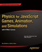
We shall also use vector equivalents of the preceding quantities and formulas. For example, the angular velocity is really a vector ω with a direction perpendicular to the plane of rotation and with an orientation as shown in Figure 13-1. The angular acceleration, as the derivative of the angular velocity, is therefore also a vector α.
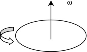
Figure 13-1. Angular velocity as a vector
Rotating rigid body objects on a canvas element
How do you rotate objects on a canvas element? In Chapter 9 we did it by rotating the whole canvas. Recall that we first have to shift the canvas so that its origin is at the object’s center before doing the rotation. After rotating the canvas, we then translate the canvas back to its original location before drawing the object. If there are many objects being animated, this process has to be repeated for each object at each timestep. Surely there has to be a better way to do this.
Although you cannot rotate individual objects on a canvas element after they are drawn, you can control the orientation with which to draw them in the first place. In an animation, if you keep track of the orientation of the object, then you can redraw it with a slightly different orientation at each timestep.
To illustrate the application of this idea, let us dig out the wheel-demo.js simulation and Wheel object from Chapter 9 and make some small modifications to them. In wheel.js we add a rotation property in the constructor to keep track of the orientation of a wheel instance. The value of rotation will represent an angle in radians, with an initial value of 0:
this.rotation = 0;
Then, in the draw() method of Wheel, we modify the code that draws the spokes, as shown here in bold:
for (var n=0; n<nums; n++){
     context.moveTo(this.x,this.y);
     context.lineTo(this.x + ir*Math.cos(2*Math.PI*n/nums + this.rotation), this.y + ir*Math.sin(2*Math.PI*n/nums + this.rotation));
}
With this modification, the draw() method adds the rotation of the wheel instance to the angle at which it draws each spoke.
Next we modify wheel-demo.js from Chapter 9, calling the new file wheel-rotate.js. In that file we get rid of the lines of code in onTimer() that perform the canvas transformations:
context.save();
context.translate(wheel.x,wheel.y);
context.rotate(angle);
context.translate(-wheel.x,-wheel.y);
context.restore();
We replace these five lines with the single line:
wheel.rotation = angle;
Run the code and you’ll find it produces exactly the same animation as the one in Chapter 9. But this code is simpler, more elegant and more efficient. The performance gains may not be noticeable in this simple example, but they can be considerable if lots of rotating objects are being animated.
The Polygon object and rotating polygons
The method we used in the previous section can be adapted to rotate other types of objects besides wheels. We’ll be dealing with polygons a lot in this chapter, so let’s create a Polygon object and apply the method to it:
function Polygon(vertices,color,mass){
     if(typeof(color)==='undefined') color = '#0000ff';
     if(typeof(mass)==='undefined') mass = 1;
     this.vertices = vertices;
     this.color = color;
     this.mass = mass;
     this.x = 0;
     this.y = 0;
     this.vx = 0;
     this.vy = 0;
     this.angVelo = 0;
}

Polygon.prototype = {
     get pos2D (){
          return new Vector2D(this.x,this.y);
     },
     set pos2D (pos){
          this.x = pos.x;
          this.y = pos.y;
     },
     get velo2D (){
          return new Vector2D(this.vx,this.vy);
     },
     set velo2D (velo){
          this.vx = velo.x;
          this.vy = velo.y;
     },
     set rotation (angle){
          for (var i=0; i<this.vertices.length; i++){
               this.vertices[i] = this.vertices[i].rotate(angle);
          }
     },
     draw: function (ctx) {
          var v = new Array();
          for (var i=0; i<this.vertices.length; i++){
               v[i] = this.vertices[i].add(this.pos2D);
          }
          ctx.save();
          ctx.fillStyle = this.color;
          ctx.beginPath();
          ctx.moveTo(v[0].x,v[0].y);
          for (var i=1; i<v.length; i++){
               ctx.lineTo(v[i].x,v[i].y);
          }
          ctx.lineTo(v[0].x,v[0].y);
          ctx.closePath();
          ctx.fill();
          ctx.restore();
     }
}
The Polygon object takes three arguments: vertices, color, and mass. It is the first of those, vertices, that is of interest here. This is an array of Vector2D objects that specify the position vectors of the vertices of the polygon instance to be created. These position vectors are relative to the position of the polygon object, as specified by the x and y values. For a regular polygon, that would be at the position of its geometrical center. The draw() method draws a polygon by joining these vertices. The way the rotation property works here is different than in the Wheel object. Here a setter is used to rotate the vertices of the polygon by an angle assigned as the value of rotation. This is done using the newly created rotate() method of the Vector2D object, which rotates a vector through the angle specified as its argument (in radians). It is defined as follows:
function rotate(angle){
     return new Vector2D(this.x*Math.cos(angle) - this.y*Math.sin(angle), this.x*Math.sin(angle) + this.y*Math.cos(angle));
}
It uses some trigonometry to do that, which you can try to figure out as an exercise.
The polygon-rotate.js file gives an example of how to use the Polygon object to create a polygon and make it rotate:
var canvas = document.getElementById('canvas'),
var context = canvas.getContext('2d'),
var v = 10;       // linear velocity in pixels per second
var w = 1;        // angular velocity in radians per second
var angDispl = 0; // initial angular displacement in radians
var dt = 30/1000; // time step in seconds = 1/FPS
// create a polygon
v1 = new Vector2D(-100,100);
v2 = new Vector2D(100,100);
v3 = new Vector2D(150,0);
v4 = new Vector2D(100,-100);
v5 = new Vector2D(-100,-100);
var vertices = new Array(v1,v2,v3,v4,v5);
var polygon = new Polygon(vertices);
polygon.x = 300;
polygon.y = 300;
polygon.draw(context);
setInterval(onTimer, 1/dt);
function onTimer(evt){
     polygon.x += v*dt;
     angDispl = w*dt;
     polygon.rotation = angDispl;
     context.clearRect(0, 0, canvas.width, canvas.height);
     polygon.draw(context);
}
As you can see, this code works in the same way as the modified wheel example in the previous section, simply by updating the value of the rotation property of the polygon instance inside the time loop, without needing to invoke canvas transformations.
As pointed out at the beginning of this section, you can adapt this method to deal with other types of objects. We have implemented a variation of it in the Ball object by defining “vertices” corresponding to the end-points of the lines drawn on a Ball instance when its line property is specified as true. Take a look at the modified ball.js file in the source code for this chapter. Ball instances can then be made to rotate simply by changing their rotation property prior to drawing them, as illustrated in the ball-rotate.js example file.
The turning effect of a force: torque
Suppose a rigid body is at rest and we want to translate it (give it some linear velocity). How do we do that? We need to apply a force. But what must we do if we want to rotate it about a given axis? Again we need to apply a force. But the line of action of the force must not pass through the axis. The turning effect of a force is known as a moment or torque, and is defined as the product of the force and the perpendicular distance of its line of action from the axis (see Figure 13-2):
![]()

Figure 13-2. Definition of torque due to a force
Here, θ is the angle between the force F and the vector r from the center of rotation to the point of application of the force.
In vector form, it is the following:
![]()
Note that the vector product is not commutative, so the order in which the product is performed matters. Because the vector product of two vectors gives a vector that is perpendicular to both, if r and F are in the plane of the paper, the torque will point either into or out of the paper (see the section “Multiplying vectors: Vector or cross product” in Chapter 3 for how to work out the direction of the resulting vector).
From this definition, it is clear that the torque is zero if the line of action of the force passes through the axis. In general, a force will produce both a linear acceleration and a turning effect.
From what we have said in the previous section, you can see that if an object is free to move (without any constraints) and you apply a force on it, it will undergo both a translation and a rotation. An exception arises if the line of action of the force passes through a special point known as the center of mass of the object. In that case, the applied force produces only translation, but no rotation.
Center of mass is a general concept that applies to collections of point particles as well as to extended objects. In both cases, it represents the location at which the overall mass of the system appears to act. For a collection of point particles of mass m1, m2, … located at positions r1, r2, …, the position vector of the center of mass is given by the following formula:
So we add the products mr of the particles vectorally and divide the sum by their total mass. Using the symbol Σ, which stands for sum, we can write this formula in the following shorthand form:

For a rigid body, a generalization of this formula is used by considering the body as being composed of a continuous distribution of particles. The center of mass of a rigid body can then be computed using the calculus formula:

The denominator of this formula is simply equal to the total mass of the rigid body. The location of the center of mass will depend on the shape of the body as well as on how its mass is distributed. For objects that are symmetrical and with a uniform mass distribution, the center of mass is located at their geometrical center. For example, the center of mass of a sphere is located at its center. It is similar for other objects such as cuboids, discs, and rectangles.
The center of mass is important for two reasons. First, it provides a connection between particle dynamics and rigid body dynamics: in terms of its translational motion, a rigid body can be thought of as a particle located at its center of mass. Second, the analysis of rigid body motion is much simpler if expressed in terms of a coordinate system with the center of mass as the origin.
We said that torque is the analog of force for rotational motion: torque is the cause of angular acceleration. What is the rotational analog of mass (inertia)? This may not be obvious, but, as will be demonstrated in the next section, it is a quantity known as the moment of inertia. The moment of inertia is defined as the sum of mr2 for all the particles comprising the particle system or rigid body, where m is the mass of the particle and r is its distance from the axis of rotation. For a discrete system of particles, the definition of the moment of inertia (denoted by the symbol I) is therefore the following:
![]()
This formula tells us that the larger the mass of the particles or the greater their distance from the axis, the larger the moment of inertia.
For a continuous distribution of mass such as a rigid body, the corresponding calculus definition is the following:
![]()
Both of these formulas tell us that the moment of inertia is a property that quantifies the mass distribution in a rigid body. Using the calculus formula, one can work out the moment of inertia of a variety of regular rigid bodies in both 2D and 3D. The result is a formula in terms of the total mass and some linear dimensions of the rigid body.
For example, the moment of inertia of a hollow sphere of mass m and radius r about an axis through its center is given by the following formula:

Because the moment of inertia depends on the mass distribution, a solid sphere of the same mass m and radius r has a different moment of inertia, being given by this formula:

So a hollow sphere has a larger moment of inertia (and is therefore harder to rotate) than a solid sphere of the same mass and radius.
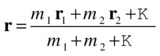
The moment of inertia also depends on the axis around which the rotation takes place. For example, the solid cylinder shown in Figure 13-3 has a moment of inertia around the x-axis and y-axis given by the following formula (where m is its mass, r is the radius of its circular cross-section and h is its height):
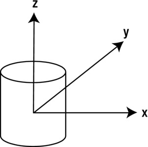
Figure 13-3. Rotation of a solid cylinder about different axes
The corresponding moment of inertia of the same cylinder around the z-axis is given by a different formula:

You can find the moments of inertia of a wide variety of 2D and 3D objects in physics or engineering textbooks and web sites.
Another important concept is that of angular momentum, which is the rotational analog of linear momentum. For a particle rotating about a center at a distance r from it, the angular momentum (denoted by the symbol L) is defined as the product of its linear momentum and the distance r:
![]()
In vector form, the angular momentum vector is the vector product of the position and momentum vectors:
![]()
Using the relationship between linear and angular velocity v = rω, gives this:
![]()
Therefore, for a collection of particles all rotating with the same angular velocity ω, the total angular momentum is given by the following:
![]()
Using the definition of moment of inertia, this gives the following result:
![]()
In vector form, it is this:
![]()
This result also applies to rigid bodies, with the appropriate calculus definition of moment of inertia.
Modeling rigid bodies
Armed with our knowledge of rigid body concepts, we can now build some basic JavaScript objects that will help us create rigid bodies.
Creating a RigidBody object
The first object we’ll create is the RigidBody object. Because a rigid body has all the properties of a particle plus more, it might make sense to “extend” the Particle object using the method emulating classical inheritance described in Chapter 4. This would be the recommended approach if you were to develop a large library with numerous objects inheriting properties from other objects. But in the interest of clarity we’ll just modify the code for the Particle object in particle.js and save it as rigidbody.js.
In fact, our RigidBody object will just replace the charge property of the Particle object by the im property, which represents moment of inertia (with a default value of 1). So here is the RigidBody object code:
function RigidBody(mass,momentOfInertia){
     if(typeof(mass)==='undefined') mass = 1;
     if(typeof(momentOfInertia)==='undefined') momentOfInertia = 1;
     this.mass = mass;
     this.im = momentOfInertia;
     this.x = 0;
     this.y = 0;
     this.vx = 0;
     this.vy = 0;
}

RigidBody.prototype = {
     get pos2D (){
          return new Vector2D(this.x,this.y);
     },
     set pos2D (pos){
          this.x = pos.x;
          this.y = pos.y;
     },
     get velo2D (){
          return new Vector2D(this.vx,this.vy);
     },
     set velo2D (velo){
          this.vx = velo.x;
          this.vy = velo.y;
     }
}
The position of a rigid body instance will always be taken to be that of its center of mass, and is specified by the x and y properties or equivalently by the pos2D property.
Extending the RigidBody object
Like Particle, the RigidBody object has no graphics. To do anything with it in practice, you need to “extend” it and include some graphics. Let’s create a couple of examples that we will use later in this chapter.
Just as RigidBody replaced the charge property in Particle by the im (moment of inertia) property, we do the same with the Ball object and call the new object BallRB. So the constructor of BallRB looks like this:
function BallRB(radius,color,mass,momentOfInertia,gradient,line){}
All the parameters are optional, with default values of 20, '#0000ff', 1, 1, false, and false respectively.
Next we create a PolygonRB object in a similar way to the BallRB class, essentially by just adding a moment of inertia property to Polygon. The parameters in the constructor of this object are therefore as follows:
function PolygonRB(vertices,color,mass,momentOfInertia){}
As with the Polygon object, vertices is an array of Vector2D values that corresponds to the locations of the vertices relative to the position of the PolygonRB instance, hence relative to the center of mass of the polygon.
Like Polygon, the PolygonRB object draws a polygon with a fill of the specified color. The order in which the vertices are specified is important. The code draws the polygon by joining the vertices in the specified order, so that different shapes result from different orderings of the vertices.
Using the rigid body objects
The file rigid-body-test.js contains code that demonstrates the use of these rigid body classes. This code produces a BallRB object rotated by 45° and a square PolygonRB object and makes them rotate at different rates and in opposite senses. The square is also made to move slowly to the right as it rotates. Comparing this example with the earlier rotating polygon in polygon-rotate.js shows that we haven’t done anything substantially new yet— we haven’t made use of the moment of inertia property of either BallRB or PolygonRB. To do this we need to implement rotational dynamics into our simulations. But before we can do that we need a bit more theory.
Rotational dynamics of rigid bodies
Having developed relevant rotational motion concepts in analogy with their linear counterparts, we are now in a position to formulate the laws of rotational dynamics. Let’s start with the most important one: the rotational equivalent of Newton’s second law of motion.
Newton’s second law for rotational motion
Consider a rigid body that is rotating about an axis under the action of a force F (which produces a torque T), as shown in Figure 13-4.
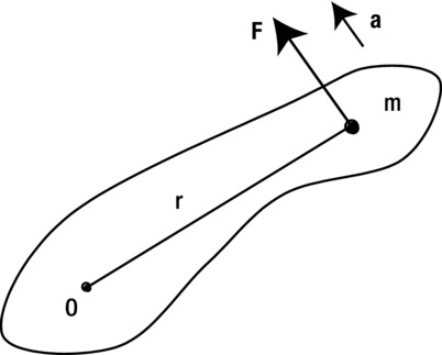
Figure 13-4. A rotating rigid body
Let’s think of the rigid body as being composed of little particles, each of mass m, each undergoing a tangential acceleration a (ignore any radial acceleration, which does not contribute to rotation). Then, applying Newton’s second law to such a particle gives the following:
![]()
Recalling the formula relating the tangential acceleration to the angular acceleration, a = rα, we can write the previous formula as follows:
![]()
Therefore, the torque T = Fr on the particle is obtained by multiplying the previous formula by r to give this:
![]()
To get the total torque on the rigid body, we sum the torques on each particle to give the following formula:
![]()
Strictly speaking, we should use an integral rather than a discrete sum for a rigid body, but the reasoning and final answer are the same because an integral is nothing but a continuous sum. So we’ll use the simpler discrete summation notation here.
Because all points on a rigid body have the same angular acceleration, α is a constant, and we can take it out of the sum. Recognizing Σ mr2 as the moment of inertia I, we then obtain the following final result:
![]()
In vector form, it is this:
![]()
This formula is the equivalent of Newton’s second law F = ma for rotational motion, with torque, moment of inertia, and angular acceleration replacing force, mass, and linear acceleration, respectively. The formula enables us to calculate the angular acceleration of a rigid body from the torque exerted on it.
As a special case, if the torque T is zero, the formula implies that the angular acceleration is also zero. This is the analog of Newton’s first law of motion.
Just as in linear motion, you can have retarding torques as well as accelerating torques. For example, you apply an accelerating torque to make a merry-go-round spin. It then slows down and stops because of the action of a retarding torque applied by friction.
Rigid bodies in equilibrium
In Chapter 4, we discussed the situation of an object in equilibrium under the action of multiple forces. For example, an airplane moving at constant velocity is in equilibrium under the action of four main forces (gravity, thrust, drag, and lift). The condition for equilibrium is that the forces balance (the resultant force is zero). But for an extended object, such as a rigid body, this condition is not enough. The resultant torque must also be zero; otherwise, the object will undergo rotational acceleration.
This concept of rotational equilibrium is well illustrated with the example of a balance (see Figure 13-5).
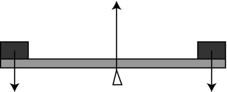
Figure 13-5. Rotational equilibrium illustrated by a balance
Assuming that the balance is in equilibrium, the downward force exerted by the combined weights on either side of the pivot is balanced by the upward contact force exerted by the pivot. Also, the clockwise torque or moment generated by one weight is balanced by the counterclockwise torque generated by the other weight: this is known as the principle of moments. In vector terms, one of the torques points out of the paper and the other points into the paper.
An example of a situation in which the resultant force may be zero and the resultant torque is not is when you turn a knob (see Figure 13-6). In that case, there are two opposite forces applied to either side of the knob. If their magnitudes are equal, they will give a zero resultant force. However, their torques will be in the same direction (into the paper) because they both generate clockwise rotations. This is an example of a couple: a pair of equal and opposite forces that have parallel non-coincident lines of action that therefore generate a resultant torque.
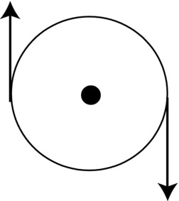
Figure 13-6. A couple
Conservation of angular momentum
Just as there is a rotational analog of Newton’s second law, rotational analogs of other laws exist, too. We shall now state these laws without proof, starting with the principle of conservation of angular momentum.
This principle states that the angular momentum of a rigid body or a system of particles is conserved if no external torque acts on it. For example, if an object is spinning at constant angular velocity, it will continue to do so unless an external torque is applied to it. That’s the reason the Earth continues to spin on its axis. On the other hand, a spinning top soon stops spinning because of opposing frictional torque.
Angular impulse-momentum theorem
The conservation of angular momentum is a special case of the angular impulse-momentum theorem. Recall the linear impulse-momentum theorem from Chapter 5. The formula expressing that theorem looks like this:
![]()
This formula tells us that the impulse applied to an object is equal to the change in momentum produced.
The rotational analog of the previous equation is obtained by taking the vector product of r with each side of the equation to give the following (because T = r × F and L = r × p):
![]()
In other words, the angular impulse applied to an object is equal to the change in angular momentum it produces. Recall that, for a rigid body, angular momentum L = I w. This result will be useful when we consider collisions between rigid bodies.
If the torque T = 0, the theorem gives ΔL = 0, angular momentum conservation. Therefore, the principle of angular momentum conservation is a special case of the angular impulse-momentum theorem as stated earlier.
Because a rigid body can rotate as well as translate, there is kinetic energy associated with rotational motion in addition to the kinetic energy associated with linear motion. Recall that the linear kinetic energy is given by the following formula:

We said that the moment of inertia is analogous to mass, and angular velocity is analogous to linear velocity. Therefore, you might not be surprised to learn that rotational kinetic energy is given by the following formula:

Therefore, the total kinetic energy of a rigid body is the sum of these two kinetic energies.
Work-energy theorem for rotational motion
In an analogy of the work done by a force, the work done by a torque is equal to the product of the torque and the angular displacement it produces:
![]()
We can then apply the work-energy theorem (see Chapter 4) to the case of rotational motion, concluding that the work done by a torque is equal to the change in rotational kinetic energy that it produces:
![]()
In that case, the kinetic energy is given by Ek = ½ Iω2.
Simulating rigid body dynamics
We are now ready to implement rigid body dynamics in code. To do this, we will need to modify relevant bits of the animation loop code that we have so far been using in this book.
Modifying the animation loop to include rotational dynamics
The animation code needs to be modified in a straightforward way to include torque and angular acceleration, in exact analogy to force and linear acceleration. The following listing shows typical code to achieve this, with the added bits highlighted in bold:
function moveObject(obj){
     obj.pos2D = obj.pos2D.addScaled(obj.velo2D,dt);
     obj.rotation = obj.angVelo*dt;
     context.clearRect(0, 0, canvas.width, canvas.height);
     obj.draw(context);
}
function calcForce(obj){
     force = Forces.zeroForce();
     torque = 0;
}
function updateAccel(obj){
     acc = force.multiply(1/obj.mass);
     alp = torque/obj.im;
}
function updateVelo(obj){
     obj.velo2D = obj.velo2D.addScaled(acc,dt);
     obj.angVelo += alp*dt;
}
In this code, torque represents the magnitude of the torque and alp represents the magnitude of the angular acceleration. Hence, they are both numbers rather than Vector2D objects like the corresponding force and acc variables. The reason we only represent the magnitudes of the torque and angular acceleration is that in the 2D examples that we’ll consider, the rotation can only take place in the x–y plane (there is only one plane), so the direction of any associated angular velocity, angular acceleration, and torque will always be in a hypothetical third dimension that sticks either into or out of that plane. The sign of the relevant quantity will determine which way it points.
A simple test
Let’s test the new rotational dynamics code with a simple example. In rigid-body-dynamics.js, we create a square rigid body using the PolygonRB object and then subject it to an imposed torque. The setup code in the init() method looks like this:
function init() {
     var v1 = new Vector2D(-100,100);
     var v2 = new Vector2D(100,100);
     var v3 = new Vector2D(100,-100);
     var v4 = new Vector2D(-100,-100);
     var vertices = new Array(v1,v2,v3,v4);
     rigidBody = new PolygonRB(vertices);
     rigidBody.mass = 1;
     rigidBody.im = 5;
     rigidBody.pos2D = new Vector2D(200,200);
     rigidBody.velo2D = new Vector2D(10,0);
     rigidBody.angVelo = 0;
     rigidBody.draw(context);
     t0 = new Date().getTime();
     animFrame();
}
The body’s mass and moment of inertia are set and its velocity and angular velocity are initialized. The subsequent animation code looks like this:
function animFrame(){
     animId = requestAnimationFrame(animFrame,canvas);
     onTimer();
}
function onTimer(){
     var t1 = new Date().getTime();
     dt = 0.001*(t1-t0);
     t0 = t1;
     if (dt>0.2) {dt=0;};
     move();
}
function move(){
     moveObject(rigidBody);
     calcForce(rigidBody);
     updateAccel(rigidBody);
     updateVelo(rigidBody);
}
function moveObject(obj){
     obj.pos2D = obj.pos2D.addScaled(obj.velo2D,dt);
     obj.rotation = obj.angVelo*dt;
     context.clearRect(0, 0, canvas.width, canvas.height);
     obj.draw(context);
}
function calcForce(obj){
     force = Forces.zeroForce();
     force = force.addScaled(obj.velo2D,-kLin); // linear damping
     torque = 1;
     torque += -kAng*obj.angVelo; // angular damping
}
function updateAccel(obj){
     acc = force.multiply(1/obj.mass);
     alp = torque/obj.im;
}
function updateVelo(obj){
     obj.velo2D = obj.velo2D.addScaled(acc,dt);
     obj.angVelo += alp*dt;
}
As you can see in the calcForce() method, a torque of magnitude 1 unit is applied at each timestep. If that was all that was done, the square would undergo continuous angular acceleration, rotating faster and faster. Therefore, an angular damping term proportional to the angular velocity is also applied to limit its angular velocity. A linear damping term is also added to the force. The values of the corresponding damping factors kLin and kAng are set to 0.05 and 0.5 respectively.
If you run the simulation, you will find that the square translates to the right while rotating in a clockwise sense. As time progresses, its linear velocity decreases until it stops (because there is no driving force but a retarding force proportional to its velocity), whereas its angular velocity increases to a constant value (you can check this by tracing the angular velocity at each timestep). The latter happens because the applied torque of 1 unit tends to increase the angular velocity whereas the angular damping term grows as the angular velocity increases. Therefore, at some point the damping term balances the applied torque and rotational equilibrium is achieved (as well as linear equilibrium). It’s the equivalent of terminal velocity for rotational motion. You can calculate the “terminal angular velocity” in the following way.
Start with the equation of angular motion relating torque and angular acceleration:
![]()
In the present simulation, because there is a driving torque of 1 unit and a retarding torque proportional to the angular velocity, the resultant torque T is given by this:
![]()
Using the previous equation of motion then gives the following:
![]()
At equilibrium, the angular acceleration α is zero. Therefore, the left side of this equation is zero. Rearranging gives the following result:
![]()
This is the “terminal” angular velocity. Using the value of k = 0.5 in the code gives a value of 2 for this angular velocity. If you trace the body’s angular velocity at each timestep in the simulation you will find that it indeed converges to this value.
Experiment by changing the mass and moment of inertia of the body. You will find that they affect the time it takes to achieve linear and rotational equilibrium respectively, but do not affect the final linear velocity (0) or final angular velocity (2).
We can now simulate rotational dynamics! Let’s build some more interesting examples.
Example: a simple wind turbine simulation
In this example we’ll simulate the motion of more than one rigid body. The objects we’ll simulate are wind turbines. So we start by creating a turbine function that makes use of PolygonRB to draw a filled polygon consisting of six vertices. Three of the vertices lie equidistant along the circumference of an inner circle, and the other three lie on an outer circle. The vertices on the inner and outer circle alternate so that the resulting Polygon looks like a wind turbine. The turbine function takes five parameters corresponding to the radius of the inner and outer circles (ri and ro), the turbine color (col), its mass (m) and moment of inertia (im), and it looks like this:
function turbine(ri,ro,col,m,im){
     var vertices = new Array();
     for (var i=0; i<3; i++){
          var vertex = getVertex(ro,i*120);
          vertices.push(vertex);
          vertex = getVertex(ri,i*120+60);
          vertices.push(vertex);
     }
     return new PolygonRB(vertices,col,m,im);
}
The function getVertex() returns the vertex position as a Vector2D object given its distance from the turbine center and its angle from the horizontal:
function getVertex(r,a){
     a *= Math.PI/180;
     return new Vector2D(r*Math.cos(a),r*Math.sin(a));
}
In the file wind-turbines.js we use the turbine function to create three turbines of different sizes, as shown in Figure 13-7.
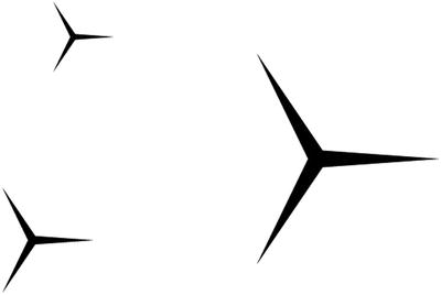
Figure 13-7. Creating wind turbines!
This is done in the init() method of wind-turbines.js:
function init() {
     turbines = new Array();
     var turbine1 = turbine(4,50,'#000000',1,1);
     turbine1.pos2D = new Vector2D(200,150);
     turbines.push(turbine1);
     var turbine2 = turbine(6,75,'#000000',2.25,5);
     turbine2.pos2D = new Vector2D(150,400);
     turbines.push(turbine2);
     var turbine3 = turbine(12,150,'#000000',9,81);
     turbine3.pos2D = new Vector2D(500,300);
     turbines.push(turbine3);
     addEventListener('mousedown',onDown,false);
     t0 = new Date().getTime();
     animFrame();
}
The code assigns different masses and moments of inertia to the turbines. The masses are assigned in proportion to the square of the outer radius of the turbines (treating them as two-dimensional), while the moments of inertia are in proportion to the fourth power of the outer radius (because I is proportional to mr2, and m is proportional to r2). The masses are really irrelevant because the turbines will only rotate. Changing their values to anything else won’t make any difference to the rotation. But we set appropriate values for physical consistency.
Part of the animation code is shown here:
function move(){
     context.clearRect(0, 0, canvas.width, canvas.height);
     for (var i=0; i<turbines.length; i++){
          var windTurbine = turbines[i];
          moveObject(windTurbine);
          calcForce(windTurbine);
          updateAccel(windTurbine);
          updateVelo(windTurbine);
     }
}
function moveObject(obj){
     obj.pos2D = obj.pos2D.addScaled(obj.velo2D,dt);
     obj.rotation = obj.angVelo*dt;
     obj.draw(context);
}
function calcForce(obj){
     force = Forces.zeroForce();
     torque = tq;
     torque += -k*obj.angVelo; // angular damping
}
function updateAccel(obj){
     acc = force.multiply(1/obj.mass);
     alp = torque/obj.im;
}
function updateVelo(obj){
     obj.velo2D = obj.velo2D.addScaled(acc,dt);
     obj.angVelo += alp*dt;
}
This code should look familiar from the previous example. In the calcForce() method, we specify a zero resultant force and a driving torque of magnitude tq as well as an angular damping term proportional to the angular velocity. The value of the torque magnitude tq is controlled by mouse-click event handlers: if the mouse is pressed, tq is given a value tqMax (which is 2 by default); if not, it has a value of 0. This means any time the mouse is clicked, a constant driving torque is applied to each turbine; otherwise, the driving torque is zero.
function onDown(evt){
     tq = tqMax;
     addEventListener('mouseup',onUp,false);
}
function onUp(evt){
     tq = 0;
     removeEventListener('mouseup',onUp,false);
}
Run the simulation and click anywhere on the canvas. What do you see? The smallest turbine starts turning almost immediately while the largest one only starts turning slowly. This illustrates the concept of rotational inertia: a rigid body with a larger moment of inertia will accelerate less than one with a smaller moment of inertia for the same torque. This is, of course, nothing but the consequence of T = Iα. Similarly, if you stop pressing the mouse, the smallest turbine will stop quickly; the largest one will stop only after a long time.
While this simulation captures the basic dynamics of a rotating turbine, more work is needed to make a more realistic simulation of how it operates in practice with wind forcing. For example, the torque and damping coefficient for each turbine will depend on characteristics such as its surface area. Wind modeling is another subject in its own right. We won’t dwell on these complicating factors; instead we'll move to another example!
Example: Rolling down an inclined plane
Rolling involves an interesting and particularly instructive application of rotational dynamics, but it can be fairly complex to understand. Therefore we’ll approach the subject through a specific example.
In Chapter 7, we simulated the motion of a ball sliding down an inclined plane. It was noted there that the ball would slide only if the incline were steeper than a certain critical angle that depends on the coefficient of static friction. The simulation worked well, but there was a major defect: the ball would not move if the angle was not high enough. This is hardly realistic; in reality balls roll down inclined planes whatever their angle of inclination!
From a particle to a rigid body simulation
We are now in a position to incorporate rolling into the ball sliding down an inclined plane simulation. But first we need to treat the ball as a rigid body instead of a particle. So let’s dig out that old code, sliding.js, and modify it to make use of our new rigid body object BallRB. The setup part of the file, rolling.js, initially looks like this:
var ball;
var r = 20; // radius of ball
var m = 1;  // mass of ball
var g = 10; // acceleration due to gravity
var ck = 0.2;  // coeff of kinetic friction
var cs = 0.25; // coeff of static friction
var vtol = 0.000001 // tolerance
// coordinates of end-points of inclined plane
var xtop = 50; var ytop = 150;
var xbot = 450; var ybot = 250;
var angle = Math.atan2(ybot-ytop,xbot-xtop); // angle of inclined plane
var acc, force;
var alp, torque;
var t0, dt;
var animId;

window.onload = init;

function init() {
     // create a ball
     ball = new BallRB(r,'#0000ff',m,0,true,true);
     ball.im = 0.4*m*r*r; // for solid sphere
     ball.pos2D = new Vector2D(50,130);
     ball.velo2D = new Vector2D(0,0);
     ball.draw(context);
     // create an inclined plane
     context_bg.strokeStyle = '#333333';
     context_bg.beginPath();
     context_bg.moveTo(xtop,ytop);
     context_bg.lineTo(xbot,ybot);
     context_bg.closePath();
     context_bg.stroke();
     // make the ball move
     t0 = new Date().getTime();
     t = 0;
     animFrame();
}
This is similar to the code in Chapter 7, and it produces the setup shown in Figure 13-8. In addition, we have specified the mass and moment of inertia of the ball. For the latter, we are using the formula for the moment of inertia of a solid sphere (I = 2mr2/5), assuming we are simulating a solid spherical ball.
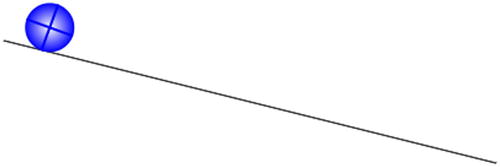
Figure 13-8. A ball rolling down an inclined plane
The animation part of the code is standard, except for the calcForce() method, which initially looks like this (we will soon modify it):
function calcForce(){
     var gravity = Forces.constantGravity(m,g);
     var normal = Vector2D.vector2D(m*g*Math.cos(angle),0.5*Math.PI-angle,false);
     var coeff;
     if (ball.velo2D.length() < vtol){  // static friction
          coeff = Math.min(cs*normal.length(),m*g*Math.sin(angle));
     }else{  // kinetic friction
          coeff = ck*normal.length();
     }
     var friction = normal.perp(coeff);
     force = Forces.add([gravity, normal, friction]);
}
If you compare this code with the corresponding calcForce() method for the sliding.js example from Chapter 7, you’ll find that it does the same thing, with identical forces and parameter values. All that we’ve done so far is to replace Ball with BallRB so that we can introduce rigid body dynamics. If you were to run the code in its current form, the ball would not move, just as in Chapter 7, unless you made the incline steeper (for example, by changing the value of ybot in the setup file to 260 or more). We know that in real life the ball would roll down the slope even if it can’t slide. So what’s missing?
Simulating rolling without slipping
You might be tempted to just add a torque to calcForce() and see whether that makes the ball roll. As you can see from the last line of code, there are three forces included in the simulation: gravity, the normal force, and friction (see the force diagram in Figure 13-9). Because both gravity and the normal force act through the center of mass, they do not have any associated torque about the center of mass. Only the frictional force has a torque about the center of mass of the ball, and the magnitude of that torque is fr, where f is the magnitude of the friction force, and r is the radius of the ball.
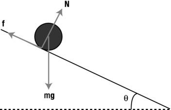
Figure 13-9. Force diagram for a ball rolling down an inclined plane
Add the following line of code after the last line in calcForce():
torque = r*friction.length();
Now run the code. What do you find? Sure the ball rotates faster and faster under the action of the torque generated by the frictional force, but it does not go anywhere! We are still missing something. Leave the torque code because it is correct. But we need to do a bit more thinking.
Let’s take another look at Figure 13-9. What else needs to change apart from accounting for the torque due to friction? The only other thing is whether the three forces are still the same with rolling. Now gravity is a fixed force that depends only on the mass of the object, so it will remain exactly the same, with magnitude mg and acting vertically downward; so will the normal force because it must still be equal and opposite to the component of gravity normal to the plane (there is no motion in that direction). Therefore, the normal force still has magnitude mg cos(θ) and acts normal to the plane, as implemented in the code.
The frictional force needs to change. Rolling friction is generally smaller than static or kinetic friction (that’s what makes the wheel such a useful invention!). At the moment, the frictional force is generally too large. So the problem really boils down to specifying the correct frictional force that will produce rolling without slipping.
The point is that the condition for rolling without slipping constrains the linear and rotational motion to “work together,” and this in turn constrains the magnitude of the frictional force. By formulating the constraint from first principles (that is, starting from basic physics laws) and working out its implications using the equations of linear and rotational motion, it is possible to deduce what the frictional force must be. Let’s do that now.
To make it easier to visualize (but without loss of generality) think of a ball or wheel of radius r that is rolling on flat ground with an angular velocity ω, as shown in Figure 13-10.
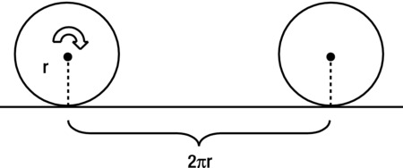
Figure 13-10. A ball or wheel rolling without slipping
If the ball or wheel rolls without slipping (let’s call this pure rolling), when it completes one revolution it has moved forward a distance equal to 2πr. It does that in a time equal to its period T, which is equal to 2π/ω (see Chapter 9). The velocity of its center of mass is given by the ratio of the distance moved to the time taken, which is therefore given by the following:
![]()
Recall that this is just the formula for the linear velocity of any point on the circumference of a circle; in pure rolling it also gives the velocity with which the whole object moves forward. This formula holds at any time, even if the angular velocity (and therefore the linear center of mass velocity) is changing. Differentiating with respect to time then gives the equivalent formula relating the linear center of mass acceleration to the angular acceleration:
![]()
This is the crucial constraint that will help us calculate the pure rolling frictional force (denoted by f). The way that force comes into play is of course through the equations of motion. Applying the linear equation of motion F = ma along the slope gives (see Figure 13-9):
![]()
Applying the angular equation of motion T = Iα gives the following:
![]()
We need to solve for the frictional force f, but we don’t know the acceleration a or the angular acceleration α. But we do have the constraint a = rα that relates them, so we can use that together with the previous equation to eliminate α and obtain the following relationship between the acceleration a and the frictional force f:
![]()
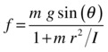
We can now substitute this into the previous equation that arose from the linear equation of motion and, after rearranging, obtain the following final result:
We can also then use the previous equation connecting a and f to deduce the following formula for the acceleration of the rolling object:
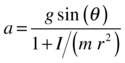
Comparing this with the acceleration of a freely falling object, g, we find that the acceleration of a rolling object is reduced by a factor that depends on the ratio I/mr2 for the body, as well as on the angle of inclination of the plane (the latter is just because we are looking at the acceleration component down the slope, rather than vertically downward).
Now that we have the formula for the frictional force for pure rolling, it’s a simple matter to include it in the code. Remove the if block of code that computes the magnitude of the friction coeff in calcForce() and replace it by the following line, which is exactly the formula for f:
coeff = m*g*Math.sin(angle)/(1+m*r*r/ball.im);
Now run the code, and you’ll have the ball rolling down the slope without slipping!
Allowing both slipping and rolling
Now increase the slope by changing the value of ybot to 850 and rerun the simulation. The slope is now very steep, but the ball will still roll down without slipping. Now we have the opposite problem: the ball does not know how to slip!
To make the simulation more realistic, we need to implement the possibility of both rolling and slipping in a simple way just by adding the following if block just after the line that computes coeff:
if (coeff > cs*normal.length()){
     coeff = ck*normal.length();
}
This imposes a limit on the maximum magnitude that the rolling friction can have; it resets the magnitude of the computed friction to the kinetic friction if it exceeds the static friction. Run the code and you’ll see that the ball now slips as it rolls down. If you change ybot back to 250 you will find that the ball undergoes pure rolling as before. In fact, you can add a console.log("slipping") line inside the if block and run the code for different values of ybot. This will tell you unequivocally when the ball is slipping. With the given parameter values, you should find that pure rolling occurs up to the value of ybot = 500, corresponding to a slope angle of approximately 41.2°.
More experiments with the simulation
A classic college physics problem is the following: suppose you release two solid cylinders, a light one and a heavy one, at the same height on a slope. Assuming that they both roll down the slope without slipping, which one will reach the bottom first? Well, you can use your simulation to find out!
First, change the value of ybot in rolling.js back to 250, so that you have pure rolling. Then change the moment of inertia formula to the following:
ball.im = 0.5*m*r*r;
This differs from the previous formula for a sphere only in the factor of 0.5; the moment of inertia of a cylinder is I = mr2/2.
Experiment with the simulation using different values for the mass and the radius of the cylinder and make a note of the time it takes for it to reach the bottom. What do you notice?
Well, counterintuitive as it may seem, you should find that the cylinder always takes the same time to reach the bottom of the slope, regardless of its mass or its radius. To see why that is so, refer to the formula for the acceleration derived in the previous subsection. Because the moment of inertia of a cylinder is given by I = mr2/2, the ratio I/mr2 that appears in that formula has the value of 0.5, giving the acceleration of a solid cylinder down the slope as
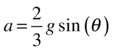
This interesting result tells us that the acceleration is completely independent of the properties of the cylinder such as mass and radius or moment of inertia: they’ve all cancelled out! So, as long as two cylinders are both solid, they should always roll down a slope at the same rate!
However, a hollow cylindrical tube has a moment of inertia given by approximately I = mr2. Going through the same calculation then gives the following acceleration:
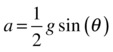
So a hollow cylindrical tube would accelerate more slowly and therefore take longer to reach the bottom of the slope.
Rigid body collisions and bouncing
In Chapter 11, we spent a considerable amount of time discussing particle collisions and bouncing. You might perhaps have felt that the math got a bit complicated then. Well, with rigid bodies, the math gets even more complicated! With rigid bodies you have to take into account both the linear motion and the rotation of the objects involved in the collision. Particles, spheres, and circular objects don’t rotate as a result of collisions (at least if we assume the collisions are frictionless). That’s because for such objects the line of collision is always through their center of mass (see Figure 13-11), so the impulsive force due to collision does not generate torque.
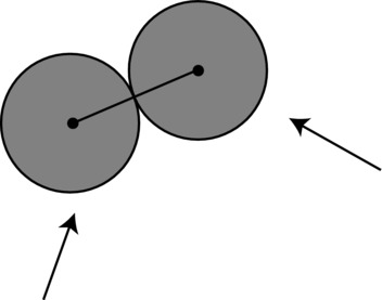
Figure 13-11. Colliding spheres
For an object with a more complicated shape, this won’t be true in general. As with a sphere, the line of collision is normal to the surface of an object, but it may not pass through the center of mass of the object (see Figure 13-12). Hence, a torque about the center of each of the colliding objects is generated in this case, causing them to rotate.

Figure 13-12. Collision between two rigid bodies of arbitrary shape
The task of collision resolution in this more general case is therefore to calculate the final linear velocities v1f and v2fand angular velocities ω1f and ω2f of the two objects, given their initial linear velocities v1i and v2i and angular velocities ω1i and ω2i (the objects could already be rotating before the collision) just before the impact. That is what we shall do in this section.
Linear impulse due to collision
The linear velocities v1i, v2i, v1f, and v2f are the initial and final linear velocities of the center of mass of the two colliding rigid bodies (denoted by the subscript 1 and 2, respectively). The angular velocities ω1i, ω2i, ω1f, and ω2f are the corresponding angular velocities about the respective center of mass of each rigid body.
The starting point is to apply the impulse-momentum theorem:
![]()
Let’s denote the impulse FΔt by the symbol J. Then, applying the impulse-momentum theorem to each rigid body and remembering that they experience equal and opposite impulse, we can write the following equations:
![]()
![]()
We note in passing that together these two equations imply the following equation:
![]()
This is nothing but conservation of momentum, as we saw in Chapter 11. We used this equation together with the one for the coefficient of restitution CR to obtain the final velocities v1f and v2f (denoted therein by v1 and v2) in terms of the initial velocities (denoted therein by u1 and u2). Refer to the section “Calculating velocities after an inelastic collision” in Chapter 11. Here the situation is more complicated because we also have the angular velocities to worry about, and we need to proceed via a slightly different route.
The approach we’ll adopt is to express the final velocities in terms of the impulse J and then to work out what J is. For the linear velocities, this is simply a matter of rearranging the previous equations involving J to obtain the following:
![]()
![]()
As with particle collisions, we can supplement these equations with one involving a coefficient of restitution. In the particle case, the coefficient of restitution was equal to the negative ratio of the relative normal velocities of the colliding particles before and after the collision. One might be tempted to assume the same here, using the linear velocities of the center of mass of each particle. But, in fact, the relevant velocities in this case are the linear velocities of the points of contact on each body normal to the contact surfaces. Referring again to Figure 13-12, these are the velocities at the point P where the two rigid bodies make contact. Let’s denote these velocities by vp1 and vp2. They are each given by the vector sum of the center of mass velocity and the velocity at the point P due to rotation about the center of mass.
So we have the following equations:
![]()
![]()
These equations are valid at any time and, in particular, just before and just after the collision. Hence, they can be written with the “i” and “f” superscripts we have used before. The vectors rp1 and rp2, which are the position vectors of the point P relative to the center of mass of each body, are the same during that brief interval, so they do not require these superscripts.
The relative velocities before and after the collision are given by the following:
![]()
![]()
The coefficient of restitution is then given by the negative ratio of the normal components of these relative velocities (where n is the unit normal vector):
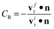
The problem is that this involves the final angular velocities as well, which we don’t know. So we need to solve for the angular velocities simultaneously. That means we need more equations. The extra equations come from applying the angular impulse-momentum theorem.
Angular impulse due to collision
Let’s now apply the angular impulse-momentum theorem:
![]()
Because T = r × F and L = Iω, this is equivalent to the following:
![]()
Applying this to each body and again remembering that they experience equal and opposite impulses gives us the following equations:
![]()
![]()
These equations can be rearranged to give the final angular velocities in terms of the initial angular velocities and the impulse:
![]()
![]()
The only thing we need now is the impulse J, and we can then obtain both the linear and angular velocities.
The final result
It is possible to solve all of the preceding equations together to obtain an expression for the impulse J. We’ll spare you the detailed algebra and just provide the final answer. Writing J = Jn, where J is the magnitude of the impulse, and n is the unit normal vector as before (because the impulse is along the direction of the normal), we obtain the following expression for the magnitude of the impulse:
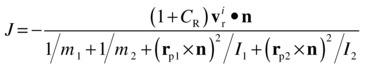
In the preceding equation, the square of each of the cross product terms (which are vector quantities) refers to taking the dot product with itself.
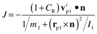
In the case in which the second rigid body is an immovable object, such as a wall, we can make m2 and I2 infinite in the previous equation (which eliminates the terms involving them). Note that the relative velocity vri in that case is just the velocity vip1 of point P on body 1. We then end up with the following:
For easy reference, let’s repeat the equations that allow you to then calculate the final linear and angular velocities:
![]()
![]()
![]()
![]()
In the case of the second object being an immovable wall, v2f and ω2f are zero.
Having been through that complex-looking math, you’ll be glad to know that the previous formulas are not actually very hard to code. In coding terms, the trickier aspects of simulating rigid body collisions are probably those of collision detection and repositioning, which are equally important and require careful consideration when creating realistic simulations.
Note that these equations are valid for collisions between rigid bodies of any shape. In the examples we will put together shortly, we are going to consider polygons. In that case, the most common collision event is the collision of a vertex of one polygon with an edge of another. The line of collision is then the normal to the relevant edge. But collisions between the vertices of two polygons are also quite common, and it is important to have a method to handle them. Other less-common collision scenarios include two vertices of an object hitting two different objects at the same time.
To avoid complications associated with these different collision scenarios and the collision detection and handling methods needed to deal with them, we will start with a simple example of a single polygon bouncing off a floor. This will allow us to focus on implementing the collision resolution method that was developed in the preceding sections. Afterward we will build a more complex simulation involving multiple colliding and bouncing objects, which will require us to confront some of the trickier issues mentioned here.
Example: Simulating a single bouncing block
We will now build a simple simulation of a rectangular block bouncing off a floor, so that we have a single movable object. The setup code for this simulation, rigid-body-bouncing.js, looks like this:
var block;
var wall;
var m = 1;
var im = 5000;
var g = 20;
var cr = 0.4;
var k = 1;
var acc, force;
var alp, torque;
var t0, dt;
var animId;

window.onload = init;

function init() {
     // create a block
     block = makeBlock(100,50,'#0000ff',m,im);
     block.rotation = Math.PI/4;
     block.pos2D = new Vector2D(400,50);
     block.draw(context);
     // create a wall
     wall = new Wall(new Vector2D(100,400),new Vector2D(700,400));
     wall.draw(context_bg);
     // make the block move
     t0 = new Date().getTime();
     animFrame();
}
function makeBlock(w,h,col,m,im){
     var vertices = new Array();
     var vertex = new Vector2D(-w/2,-h/2);
     vertices.push(vertex);
     vertex = new Vector2D(w/2,-h/2);
     vertices.push(vertex);
     vertex = new Vector2D(w/2,h/2);
     vertices.push(vertex);
     vertex = new Vector2D(-w/2,h/2);
     vertices.push(vertex);
     return new PolygonRB(vertices,col,m,im);
}
We create a rectangular block as a PolygonRB instance and a floor object using the Wall class in Chapter 11. The block is given a moment of inertia of 5000 and an initial orientation of π/4 radians (45°).
The animation part of the code is fairly standard, with an unremarkable looking calcForce() method:
function calcForce(obj){
     force = Forces.constantGravity(m,g);
     torque = 0; // no external torque since gravity is the only force
     torque += -k*obj.angVelo; // damping
}
The calcForce() method prescribes gravity as the only force on the block and specifies a zero external torque because gravity does not generate torque about its center of mass. We do include a damping torque, though, the magnitude of which is controlled by the damping parameter k (which you can set to zero if you wish).
The really new physics in the code is contained in the checkBounce() method, which is called from the move() method at each timestep, and looks like this:
function checkBounce(obj){
     // collision detection
     var testCollision = false;
     var j;
     for (var i=0; i<obj.vertices.length;i++){
          if (obj.pos2D.add(obj.vertices[i].rotate(obj.rotation)).y >= wall.p1.y){
               if (testCollision==false){
                    testCollision = true;
                    j = i;
               }else{ // that means one vertex is already touching
                    stop(); // block is lying flat on floor, so stop simulation
               }
          }
     }
     // collision resolution
     if (testCollision == true){
          obj.y += obj.pos2D.add(obj.vertices[j].rotate(obj.rotation)).y*(-1) + wall.p1.y;
          var normal = wall.normal;
          var rp1 = obj.vertices[j].rotate(obj.rotation);
          var vp1 = obj.velo2D.add(rp1.perp(-obj.angVelo*rp1.length()));
          var rp1Xnormal = rp1.crossProduct(normal);
          var impulse = -(1+cr)*vp1.dotProduct(normal)/(1/obj.mass + rp1Xnormal*rp1Xnormal/obj.im);
          obj.velo2D = obj.velo2D.add(normal.multiply(impulse/obj.mass));
          obj.angVelo += rp1.crossProduct(normal)*impulse/obj.im;
          testCollision = false;
     }
}
As you can see, the code looks surprisingly short given the apparent complexity of the preceding discussion of the theory. The code is split into two parts, one specifying the collision detection and the other the collision resolution. The collision detection code loops over the vertices of the block and tests to see whether any of them is lower than the floor using the following condition:
if (obj.pos2D.add(obj.vertices[i].rotate(obj.rotation)).y >= wall.p1.y){}
This line might look a bit complicated, so let’s break it down. First the easy bit: wall.p1.y just gives the y position of the wall. Next, obj.vertices[i] is the position vector of the vertex currently being tested relative to the center of mass of the block. You have already encountered the rotate() method of the Vector2D object earlier in this chapter.
We are therefore rotating the position vector of the current vertex through an angle equal to the angular displacement obj.rotation of the block to account for the block’s orientation. Then we add this to the block’s (center of mass) position. We do this because we need the position vector of the vertex in the canvas coordinate system, not in the center of mass coordinate system. Finally, we test whether the y component of this vector is greater than the y location of the wall. If it is, a collision is detected, and the Boolean parameter testCollision is set to true and the index of the vertex is stored in the variable j. But this is only done provided testCollision is currently false (another collision has not already been detected in the same timestep). If testCollision was already true, that means another vertex is already in collision with the floor. Physically, it means that the block is now lying flat on the floor. The reasonable thing to do then is to stop the simulation. We do this using the stop() method, which stops the animation loop:
function stop(){
     cancelAnimationFrame(animId);
}
The collision resolution code executes if a collision is detected (if testCollision is true). The first line repositions the block by simply moving it up by the amount that it fell below the wall. The next few lines of code simply implement the equations given at the end of the last section and should be straightforward to follow. The only subtlety is the use of the crossProduct() method, which is another newly created method of the Vector2D class defined as follows:
function crossProduct(vec) {
     return this.x*vec.y - this.y*vec.x;
}
This might confuse you if you recall that the cross product of two vectors is only supposed to exist in 3D and to be itself a vector. Because our simulation is in 2D, we’ve defined the analog of the cross product, but can only give its magnitude because the cross product of two vectors should be perpendicular to both and should therefore need a third dimension to exist. The bottom line is that this trick enables us to use the formulas involving vector products in the last section pretty much as they are, as long as we keep in mind that it will only give us the magnitude of the cross product (which, in fact, is all that we need in those formulas).
There is not much more to say about this simulation. Run it and enjoy! See Figure 13-13 for a screenshot. As usual, try out the effects of changing the parameters like the moment of inertia, the coefficient of restitution, and the angular damping factor. As an additional exercise, try replacing the rectangle with another polygon, such as a triangle or a pentagon.
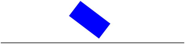
Figure 13-13. A falling block bouncing off a floor
As discussed earlier, with multiple blocks colliding together, care is needed to detect collisions between the objects and then keep them apart. So let’s spend some time discussing how they are applied in a specific example—a group of polygons with different sizes and orientations dropped from a height so that they fall onto and bounce off a floor, colliding with one another as they do so.
Figure 13-14 illustrates the most common scenario when a vertex P of one block (object 1) collides with an edge of another (object 2). At the moment of collision detection, P is inside the second polygon. If you consider the position vectors of the vertices of the second polygon relative to P, they should all have positive dot products with the normal from P to the side adjacent to them (by convention, we’ll consider the side that is in a counterclockwise direction from the relevant vertex). So if you test all these dot products and any one of them is negative, you know that no collision has taken place. You could also do a weaker test first by seeing whether the distance between the centers of mass of the two objects is larger than the distance to their farthest vertices. If so, you don’t have to bother doing the more detailed collision detection test.
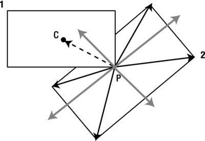
Figure 13-14. Vertex-edge collision between two polygons
To reposition an object after a vertex-edge collision, you simply move it back along the normal to the edge where the collision took place by an amount equal to the perpendicular distance from the point P to the relevant edge. The correct normal is determined by checking which one has the minimum angle with the position vector of P relative to the center of mass of object 1 (refer to Figure 13-14).
Another scenario is when a vertex of one object collides with a vertex of another. You might think that would be a rare event, but it tends to happen more often than you’d think. For example, a vertex of one polygon can slide along an edge of another until it hits the vertex at the end. In the case of vertex-vertex collisions, a simple collision detection method is to check for the distance between two vertices; if it’s smaller than a certain amount (let’s say 1 pixel), that’s counted as a collision.
We apply these methods in our example simulation. The code for the simulation is in the file rigid-body-collisions.js. This code produces a number of polygons of different sizes and orientations and assigns them masses proportional to their areas and moments of inertia based on their masses and dimensions. A Wall object is also produced to represent the floor. We won’t list all the code here, but only show the amended move() method so you get an idea of the main logic:
function move(){
     context.clearRect(0, 0, canvas.width, canvas.height);
     for (var i=0; i<blocks.length; i++){
          var block = blocks[i];
          checkWallBounce(block);
          for(var j=0;j<blocks.length;j++){
               if(j!==i){
                    checkObjectCollision(block,blocks[j]);
               }
          }
          moveObject(block);
          checkWallBounce(block);
          calcForce(block);
          updateAccel(block);
          updateVelo(block);
     }
}
As in the previous simulation, there is only gravity as an external force on each object and no external torque, so that calcForce() is the same as before. At each timestep, the checkWallBounce() method checks whether the current object is colliding with a wall and handles the collision if necessary. This method is in essence very similar to the code we saw in the previous example for detecting and resolving wall collisions. Then the checkObjectCollision() method sees whether the current object is colliding with any other object and resolves the collision if it takes place. The collision resolution code is along the same lines as that of the wall collision, but of course using the corresponding formulas for two-body collisions. The rest of the code in checkObjectCollision() detects any vertex-side or vertex-vertex collisions between two objects and repositions them according to the methods described previously. See the source code in the file rigid-body-collisions.js for the detailed implementation.
If you run the code you will find that the simulation generally works well, correctly handling the collision scenarios it is designed to detect. But because we kept the simulation simple, you may notice some problems every now and then, especially when objects get crowded and multiple collisions are involved. The problems can get worse if higher velocities are involved; for example, if g is increased. You could improve the simulation by devising methods to handle more of these possible collision scenarios. You could also introduce friction to make it look more realistic at the moment the blocks slide along the floor once they have settled due to the lack of friction. Figure 13-15 shows a screenshot of the simulation.
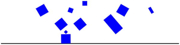
Figure 13-15. The multiple colliding blocks simulation
You now know how to simulate rigid body motion, but how do you simulate the motion of deformable bodies such as ropes and clothes, whose shapes can change? There are various ways to do that, but we’ll introduce one particular approach based on the spring physics that we covered in Chapter 8. Let’s begin with a brief recap of the main principles and formulas of spring physics and a discussion of how those principles can be applied to model deformable bodies.
The basic modeling approach is to represent a deformable extended object as a series of particles with mass joined together by virtual springs. Hence we generally refer to such models as mass-spring systems. As an illustration of the method, consider the simple one-dimensional chain of particles and springs shown in Figure 13-16.
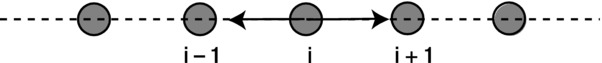
Figure 13-16. A 1D chain of particles connected by springs
Each particle experiences a spring force that depends on its distance from the adjacent particles. We can impose a certain equilibrium distance L between the particles. If two particles are closer together than the distance L, they repel; if they are farther apart than L, they attract. The length can be thought of as the natural unstretched length of the virtual spring connecting the two particles.
As described in Chapter 8, the spring force between any two particles is given by the following equation, in which k is the spring constant and x is the extension:
![]()
The magnitude of the extension x is the amount by which the spring is stretched beyond its unstretched length L. In the case of two adjacent particles connected by a spring, it is therefore equal to the distance d between the particles minus L:
![]()
In vector form, it is this:
Here d is the distance vector between the two particles. For example, the ith particle in the preceding 1D chain experiences a force due to the (i+1)th particle given by the following equation, where r is the position vector of the respective particle:
Similarly, the ith particle experiences a force due to the (i-1)th particle given by the following:
This 1D model can be extended to 2D or 3D, and each particle can then be subjected to a spring force due to more neighbors according to the previous formulas.
You also want to have damping in your mass-spring system; otherwise, the particles would just oscillate forever. The damping term is usually linear in the relative velocity with a constant coefficient c (which can be chosen to minimize the time it takes to reach equilibrium), as we discussed in Chapter 8:
![]()
In the specific context of our connected mass-spring system, the velocity vr is the velocity of the relevant particle relative to the particle exerting the force on it. Therefore, the damping force on the ith particle relative to the (i+1)th particle is given by this:
![]()
Similarly, the damping force on the ith particle relative to the (i+1)th particle is given by the following:
![]()
To get a mass-spring system to work properly, it is frequently necessary to adjust the mass, stiffness, and damping coefficient. Generally you’ll want the stiffness k to be high to reduce the stretchiness of your object. The problem is that the resulting spring system becomes more unstable, and it is not unusual to see a simulation explode before your very eyes! Let’s put together an example, and you’ll soon get to see what we mean!
Rope simulation
This example builds upon the last example in Chapter 8, where we simulated a chain of particles connected together by springs (see the “Coupled Oscillations” code). We will now make some small but significant changes to that simulation to make it behave more like a rope. The modified code is in the file rope.js and is reproduced here in full, with the most significant changes highlighted in bold:
var canvas = document.getElementById('canvas'),
var context = canvas.getContext('2d'),

var balls;
var support;
var center = new Vector2D(100,100);
var g = 10;
var kDamping = 20;
var kSpring = 500;
var springLength = 20;
var spacing = 20;
var numBalls = 15;
var drop = false;
var t0, dt;
var acc, force;
var animId;

window.onload = init;

function init() {
     // create a support
     support = new Ball(2,'#000000'),
     support.pos2D = center;
     support.draw(context);
     // create a bunch of balls
     balls = new Array();
     for (var i=0; i<numBalls; i++){
          var ball = new Ball(2,'#000000',10,0,true);
          ball.pos2D = new Vector2D(support.x+spacing*(i+1),support.y);
          ball.draw(context);
          balls.push(ball);
     }
     addEventListener('mousedown',onDown,false);
     t0 = new Date().getTime();
     animFrame();
}
function onDown(evt){
     drop = true;
     addEventListener('mouseup',onUp,false);
}
function onUp(evt){
     drop = false;
     removeEventListener('mouseup',onUp,false);
}
function animFrame(){
     animId = requestAnimationFrame(animFrame,canvas);
     onTimer();
}
function onTimer(){
     var t1 = new Date().getTime();
     dt = 0.001*(t1-t0);
     t0 = t1;
     if (dt>0.2) {dt=0;};
     move();
}
function move(){
     context.clearRect(0, 0, canvas.width, canvas.height);
     drawSpring();
     for (var i=0; i<numBalls; i++){
          var ball = balls[i];
          moveObject(ball);
          calcForce(ball,i);
          updateAccel(ball.mass);
          updateVelo(ball);
     }
}
function drawSpring(){
     support.draw(context);
     context.save();
     context.lineStyle = '#009999';
     context.lineWidth = 2;
     context.moveTo(center.x,center.y);
     for (var i=0; i<numBalls; i++){
          var X = balls[i].x;
          var Y = balls[i].y;
          context.lineTo(X,Y);
     }
     context.stroke();
     context.restore();
}
function moveObject(obj){
     obj.pos2D = obj.pos2D.addScaled(obj.velo2D,dt);
     obj.draw(context);
}
function calcForce(obj,num){
     var centerPrev;
     var centerNext;
     var veloPrev;
     var veloNext;
     if (num > 0){
          centerPrev = balls[num-1].pos2D;
          veloPrev = balls[num-1].velo2D;
     }else{
          centerPrev = center;
          veloPrev = new Vector2D(0,0);
     }
     if (num < balls.length-1){
          centerNext = balls[num+1].pos2D;
          veloNext = balls[num+1].velo2D;
     }else{
          centerNext = obj.pos2D;
          veloNext = obj.velo2D;
     }
     var gravity = Forces.constantGravity(obj.mass,g);
     var velo = obj.velo2D.multiply(2).subtract(veloPrev).subtract(veloNext);
     var damping = Forces.damping(kDamping,velo);
     var displPrev = obj.pos2D.subtract(centerPrev);
     var displNext = obj.pos2D.subtract(centerNext);
     var extensionPrev = displPrev.subtract(displPrev.unit().multiply(springLength));
     var extensionNext = displNext.subtract(displNext.unit().multiply(springLength));
     var restoringPrev = Forces.spring(kSpring,extensionPrev);
     var restoringNext = Forces.spring(kSpring,extensionNext);
     force = Forces.add([gravity, damping, restoringPrev, restoringNext]);
     if (num==balls.length-1&& drop==false){
          force = new Vector2D(0,0);
          obj.velo2D = new Vector2D(0,0);
     }
}
function updateAccel(mass){
     acc = force.multiply(1/mass);
}
function updateVelo(obj){
     obj.velo2D = obj.velo2D.addScaled(acc,dt);
}
Most of the code is unchanged from that in coupled-oscillations.js, and we therefore refer you to the relevant discussion in Chapter 8 if it is not completely obvious and you need a refresher of how it works. We’ll instead focus on the key changes.
First, notice that we are storing the velocities of the particles before and after the current one in the variables veloPrev and veloNext. They are then combined with the velocity of the current particle to give the parameter velo, which is used to compute the damping force using the Forces.damping() function. You might be wondering why we are combining the velocities in that way. Referring to the formulas for the damping force given in the previous subsection, we are adding up the damping force on the current particle relative to the two neighboring particles to give this:
![]()
The variable velo is just the combined effective velocity that results from that sum. Note that in coupled-oscillations.js we used the absolute velocity of the current particle (not the velocities relative to its neighbors) to compute the damping force on it. You might want to experiment by comparing the behavior of the simulation if you do the same here.
Another change is that we are fixing the last particle in the chain by setting the force on it and its velocity to zero, unless the Boolean parameter drop is true:
if (num==balls.length-1 && drop==false){
     force = new Vector2D(0,0);
     obj.velo2D = new Vector2D(0,0);
}
The parameter drop, initially set to false, is controlled by user interaction through the event handlers onDown() and onUp() that respond to a mousedown and mouseup event, respectively. As long as the user holds the mouse down, drop is true, and the last particle can move under the action of forces like the rest of the particles (except the first). If the mouse is released, the last particle stops wherever it is. There is a slightly modified version of the simulation in the source file rope2.js that responds in a different way to mouse clicks: when the mouse is held down, a force is applied toward the mouse with a magnitude proportional to the distance from the mouse to the last particle; the force is removed when the mouse is released. Although we refer to the first version of the simulation in the following discussion, much of it applies equally well to the modified version.
Note the values of the parameters that we specify in rope.js: gravity is 10 units, spring length is 20 pixels, and the mass of the particles is 10 units. Most importantly, note the high values used for the spring damping coefficient (20) and the spring constant (500) compared to what they were in the coupled oscillations simulation in Chapter 8, where these parameters had values of 0.5 and 10, respectively. As you experiment with this simulation, do try different values for these parameters to see how they change its behavior.
Run the simulation with the default values of these parameters. Notice how the particles fall from their initial positions under the effect of gravity, but are held together by the spring force. After some brief oscillations and slight stretching, they settle down into a curved shape that hangs down like a rope (see Figure 13-17). This is a characteristic mathematical curve known as a catenary: it’s the shape that a chain fixed at both ends naturally takes under the effect of its own weight. After it has settled down, click and hold down the mouse so that the end of the string falls down: see how the “rope” can readjust itself. Now release the mouse and notice that the rope again settles into a characteristic curve: this is a different section of the catenary.

Figure 13-17. A rope simulation
Experiment by changing the values of the parameters. First, increase the value of the spring constant kSpring to 1000. See how the rope now stretches less. You might be tempted to try a much larger value to see whether you can get an even tighter rope. Go ahead and increase kSpring to 10000 (just don’t say we didn’t warn you) and rerun the simulation. Whoops! Your rope just blew up! Welcome to numerical instability. Unfortunately, this is a common problem with mass-spring systems: they are prone to blow up, especially for high values of the spring constant. This arises because of an underlying issue with integration schemes known as numerical instability, which we’ll discuss in more detail in the next chapter.
You can similarly play with the damping coefficient kDamping and note that its value affects how quickly the oscillations stop. Problems can get nasty here, too. For example, keep kSpring at its initial value of 500 and decrease the value of kDamping to 1. The simulation seems to be well-behaved initially, apparently settling down as before. But wait a little longer and you soon start seeing little fluctuations growing and distorting the rope into something that you can’t call a rope any more.
To conclude: mass-spring systems are easy to create and fun to watch, but they can prove highly unstable in certain parameter regimes. Some steps can be taken to improve their stability, for example by using an improved integration scheme (see the next chapter), but they should be used with care.
It is fairly straightforward to extend our rope simulation to 2D to create a simple cloth simulation. Of course, to create a realistic simulation of a cloth that can bend we really need a 3D simulation, even if the cloth is 2D, to allow for movement and bending of the cloth in the third dimension. But we can quickly make a 2D version that will reproduce at least some elements of the behavior of a moving cloth. So let’s make some quick modifications to the rope simulation and create a 2D version of it. The new file is called cloth.js, the setup part of which is reproduced here:
var balls;
var rows = 10;
var cols = 15;
var refPoint = new Vector2D(120,50);
var fixedPoints = new Array(0,70,140);
var g = 10;
var kDamping = 10;
var kSpring = 100;
var kWind = 10;
var windMag = 10;
var springLength = 20;
var spacing = 20;
var w = 0;
var t0, dt;
var acc, force;
var animId;

window.onload = init;

function init() {
     // create the masses
     balls = new Array();
     for (var i=0; i<cols*rows; i++){
          var ball = new Ball(2,'#000000',10,0,true);
          var ncol = Math.floor(i/rows);
          ball.pos2D = new Vector2D(refPoint.x+ncol*spacing,refPoint.y+(i-ncol*rows-1)*spacing);
          ball.draw(context);
          balls.push(ball);
     }
     addEventListener('mousedown',onDown,false);
     t0 = new Date().getTime();
     animFrame();
}
function onDown(evt){
     w = windMag;
     addEventListener('mouseup',onUp,false);
}
function onUp(evt){
     w = 0;
     removeEventListener('mouseup',onUp,false);
}
Apart from the obvious generalization of the setup to 2D, note that we have also specified an array of points on the cloth that we want to remain fixed. In the listing, we are holding the cloth fixed at three points, giving the appearance of a piece of cloth that is hung on a line.
The calcForce() method that drives the simulation is fairly long, but it is an obvious generalization of that in the rope.js code and so we won’t list it here. Take a look at the code in the source file, though. Arguably some of the coding in that file could be done more concisely and elegantly by using arrays instead of different variables (such as extensionUp, extensionDown, and so on) that do the same thing in different directions. But the code is probably easier to understand in the current inelegant form, and the comments should also help. The main idea is that now each particle is experiencing a force due its four nearest neighbors to the left, right, up, and down, respectively. If a particle is on the edge of the cloth, it obviously does not have one or more of these forces. All the particles are subject to gravity. The other change is in terms of user interaction; clicking and holding down the mouse now applies a steady wind blowing to the right.
Run the simulation and you’ll have a hanging piece of cloth that you can blow the wind over by clicking the mouse (see Figure 13-18). Experiment with the parameters of the simulation to see what they do. For example, you can try and increase the number of particles, reduce their spacing, and so on. You might also want to increase the spring constant and see how far you can go before you tear the cloth to pieces!
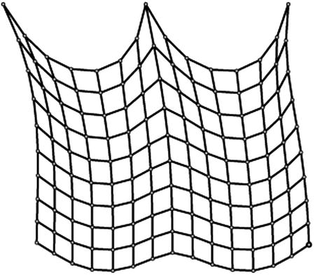
Figure 13-18. A simple cloth simulation
Needless to say, this is a very basic cloth simulation that can be enhanced in endless ways. Functionally, the most important improvement is probably to make the cloth move in 3D, but we haven’t talked about how to simulate physics in 3D yet. You could also connect each particle to more neighbors; for example, the four nearest diagonal neighbors and the next nearest neighbors up, down, left, and right. That would improve the way the cloth behaves. Visually, you could fill up the areas between the particles, as well as add texture, lighting, and so on. Over to you!
Summary
This chapter introduced rigid body dynamics and collisions, and showed you how to model deformable bodies using mass-spring systems. Needless to say, what we have covered in this chapter is only the tip of the iceberg. There are many more topics on the general subject of extended systems that we can only briefly mention here: constrained systems, forward and inverse kinematics, and Verlet systems. Some of them can provide alternative approaches to simulating both rigid bodies and deformable bodies, but we do not have the space to include a discussion of them in this book.
This chapter completes Part III. In the first chapter of Part IV, we will look at advanced numerical schemes and considerations of stability and accuracy involved in creating complex simulations.