![]()
In a nutshell, this chapter will show you how to create animated effects and simulations using systems of multiple particles. Particle systems are very popular, and a lot of creative work has been done in the animation community over the years using them. In a single chapter, we can only really scratch the surface of what is possible. Therefore, we shall content ourselves with giving you a few ideas and examples to play with and build upon.
Topics covered in this chapter include the following:
- Introduction to particle system modeling: This brief section will explain what we mean by a particle system and what is needed to set one up.
- Creating animated effects using particles: It is possible to produce some interesting animated effects such as smoke and fire using particles and some simple physics. We’ll walk you through some examples in this section.
- Particle animations with long-range forces: Particle animations don’t have to look realistic; they can be just for fun! We look at a couple of wacky examples using long-range forces such as gravity.
- Interacting particle systems: More complex particle systems include interactions between the particles. But this can get pretty computationally expensive with large numbers of particles. We give a couple of examples, discussing tricks to overcome this problem.
The approach in this chapter is to create animations that use some physics, but without necessarily being accurate simulations. Above all, this is a subject where experimentation and creativity pay dividends. Therefore, don’t be afraid to tinker and invent, even if that means breaking a few laws of physics!
Introduction to particle system modeling
Although a precise definition of a particle system probably does not exist, an attempt to define it will help to explain what we have in mind before we do anything else. In the sense in which we use the term, a particle system consists of the following elements:
- A group of particles
- Rules by which they move and change
- Rules by which they interact (if any)
This definition is very general: the said “rules” could be based on physics, artificial intelligence, biology, or any such system. It won’t come as a surprise that we’ll limit ourselves to particles moving and interacting under physical laws (with perhaps the odd tweak here and there). Therefore, the particle systems we’ll consider will animate particles according to Newton’s laws of motion under the action of a subset of the forces that we discussed in Part II of the book. The different categories of interaction between the particles can include the following:
- No mutual interaction: In this case, the particles are unaware of each other and move independently under the action of globally prescribed forces (such as external gravity). Even though this is the simplest case, quite impressive effects can be generated using non-interacting particles. We will look at several examples in the next two sections.
- Interaction by collision: Here the particles do not interact except very briefly when they collide. The collisions can be resolved using the methods given in Chapter 11. In fact, the last example in Chapter 11 showed just such a system of particles interacting via collisions.
- Short-range interactions: In this case, the particles interact only when they are close together but not necessarily touching. They can be modeled using short-range forces of a type that exists between molecules. Using such forces it is possible to model fluid effects such as the formation and fall of a liquid drop. But these simulations require more advanced methods and will not be covered in this book.
- Long-range interactions: This category involves mutual interactions between the particles at any distance, such as gravitational or electric forces between the particles. Typically, every particle experiences a force due to every other particle. Clearly the number of computations that need to be performed becomes very large pretty quickly as you increase the number of particles in the system. We look at some examples in the last section of this chapter.
- Local interactions: These interactions are intermediate between short-range and long-range; particles within a certain local neighborhood are linked and interact. Such interactions can give rise to organized systems and connected structures. Examples include mass-spring systems, which can be used to simulate deformable bodies like ropes and clothes. These particle systems are explored in Chapter 13.
So what do we need, in terms of physics and coding, to create a particle system? The answer might surprise you: not a lot beyond what we’ve already covered in the previous chapters. So there won’t be much theory in this chapter, but more on the application of principles that have already been discussed with a few extra tricks added in. That means you get to see code much sooner!
Creating animated effects using particles
One of the most common uses of particle systems is to create animated visual effects such as smoke and fire. In this section, we show you simple ways of producing some of these effects using physics-based animation. We start with a very simple example and then create a particle emitter that will allow us to create some more elaborate effects. The approach in this section is that we want to produce animations that look realistic, but that don’t have to be completely accurate.
A simple example: splash effect with particles
In this example, we will drop objects in water and then create a splash effect using particles. The objects will be balls of different sizes and will be dropped one at a time from the same height. The splash will be made from a group of Ball objects of smaller size. Let’s dive straight into the code that creates these objects. The file, downloadable from www.apress.com, is called splash.js. Here is a full listing of the code:
var canvas = document.getElementById('canvas'),
var context = canvas.getContext('2d'),
var canvas_bg = document.getElementById('canvas_bg'),
var context_bg = canvas_bg.getContext('2d'),

var drop;
var droplets;
var numDroplets = 20;
var m = 1;
var g = 20;
var vx = 20;
var vy = -15;
var wlevel = 510;
var fac = 1;
var t0,dt;
var acc, force;

window.onload = init;

function init() {
     makeBackground();
     makeDrop();
     makeDroplets();
     t0 = new Date().getTime();
     animFrame();
}
function makeBackground(){
     var horizon = 500;
     // the sea
     context_bg.fillStyle = '#7fffd4';
     context_bg.fillRect(0,horizon,canvas_bg.width,canvas_bg.height-horizon);
     // the sky
     gradient = context_bg.createLinearGradient(0,0,0,horizon);
     gradient.addColorStop(0,'#87ceeb'),
     gradient.addColorStop(1,'#ffffff'),
     context_bg.fillStyle = gradient;
     context_bg.fillRect(0,0,canvas_bg.width,horizon);
}
function makeDrop(){
     drop = new Ball(8,'#3399ff',1,0,true);
     drop.pos2D = new Vector2D(400,100);
     drop.velo2D = new Vector2D(0,100);
     drop.draw(context);
}
function makeDroplets(){
     droplets = new Array();
     for (var i=0; i<numDroplets; i++){
          var radius = Math.random()*2+1;
          var droplet = new Ball(radius,'#3399ff',m,0,true);
          droplets.push(droplet);
     }
}
function animFrame(){
     animId = requestAnimationFrame(animFrame,canvas);
     onTimer();
}
function onTimer(){
     var t1 = new Date().getTime();
     dt = 0.001*(t1-t0);
     t0 = t1;
     if (dt>0.2) {dt=0;};
     move();
}
function move(){
     context.clearRect(0, 0, canvas.width, canvas.height);
     moveObject(drop);
     checkDrop();
     for (var i=0; i<numDroplets; i++){
          var droplet = droplets[i];
          moveObject(droplet);
          calcForce(droplet);
          updateAccel();
          updateVelo(droplet);
     }
}
function moveObject(obj){
     obj.pos2D = obj.pos2D.addScaled(obj.velo2D,dt);
     if (obj.y < wlevel){// only show drops that are above water level
          obj.draw(context);
     }
}
function calcForce(obj){
     force = Forces.constantGravity(m,g);
}
function updateAccel(){
     acc = force.multiply(1/m);
}
function updateVelo(obj){
     obj.velo2D = obj.velo2D.addScaled(acc,dt);
}
function checkDrop(){
     if (drop.y > wlevel){
          for (var i=0; i<droplets.length; i++){
               var droplet = droplets[i];
               var posx = drop.x+(Math.random()-0.5)*drop.radius;
               var posy = wlevel-10+Math.random()*drop.radius;
               var velx = (Math.random()-0.5)*vx*fac;
               var vely = (Math.random()+0.5)*vy*fac;
               droplet.pos2D = new Vector2D(posx,posy);
               droplet.velo2D = new Vector2D(velx,vely);
          }
          drop.x = Math.random()*600+100;
          drop.y = 100;
          drop.radius = 4 + 8*Math.random();
          fac = Math.pow(drop.radius/8,1.5);
     }
}
Looking at the init() method first, we see that the initial setup code has been organized into three separate methods makeBackground(), makeDrop() and makeDroplets(), which respectively create the visual background, the Ball object to be dropped (named drop; think raindrop) and a group of 20 smaller Ball objects with random radii between 1 and 3 pixels. These will be the splash droplets, and they are not initially visible as they have not been drawn yet. They are put into an array called droplets. The drop is initially positioned above the water surface, at y = 100, and given a velocity of 100 px/s vertically downward.
The animation code is invoked by calling the animFrame() method from init() as usual. In the move() method the drop is animated first by invoking the moveObject() method passing drop as an argument. This makes it move at the constant downward velocity of 100 px/s specified earlier in the code. You may be wondering why we make the object fall at a constant velocity instead of making it accelerate under gravity. The answer is that if it is a raindrop, it would probably have reached terminal velocity anyway.
Next in move(), the checkDrop() method is called. This method checks whether the drop has fallen below the water level (set at 10 px below the top edge of the blue rectangle representing the body of water, to give a fake 3D effect). If that happens, the splash droplets are repositioned around the region of impact and given random velocities with an upward vertical component. The magnitude of the velocities depends on parameters vx and vy that are set initially in the code as well as on a factor fac, which is updated every time a splash occurs, as will be described shortly. The falling drop is repositioned at the initial height and at a new random horizontal location as soon as it hits the water level. Its radius is then changed to a random value between 4 and 12 pixels.
The velocity factor fac is updated according to the following formula, in which rm is the mean radius of the drop (8 pixels):

What is happening here? The idea is that the larger the drop is, the heavier its mass will be (its mass is proportional to its volume, or the cube of its radius, r3). Because the drop always has the same velocity, its kinetic energy (Ek = ½ mv2) will be proportional to its mass, and therefore to r3. A fraction of that energy will be imparted to the splash droplets, and one can therefore expect the average kinetic energy of those droplets to be proportional to r3. Because the masses of the droplets are constant, their kinetic energy is proportional to the square of their velocity. So we have the following:
![]()
Therefore, we can write the following:
![]()
This shows that we expect the droplets to have a mean velocity proportional to the radius of the falling drop raised to the power of 1.5. The previous formula for fac implements this assumption, with the value of fac being set to 1 when the radius is equal to the mean radius of 8 px.
Back in the move() method, the droplets are each animated in the for loop. They are made to fall under gravity by using the Forces.constantGravity() method in calcForce(). In moveObject() there is an if condition that draws them to the canvas only if they are below the water level; otherwise, they remain invisible.
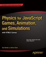
If you run the simulation, you will find that the larger the drop is, the higher the droplets will splash because of their greater initial velocities. Figure 12-1 shows a screenshot. As usual, feel free to experiment with different parameters. Of course, the visual aspects of the animation can be enhanced in many ways according to your imagination and artistic skills. We have focused on the physics and coding aspects; feel free to season the appearance to taste.
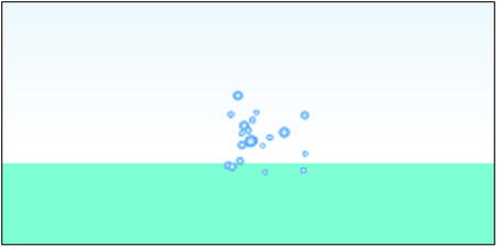
Figure 12-1. Producing a splash!
Many applications of particle systems require a continuous source of particles. This can be achieved using particle emitters. Creating a particle emitter is not difficult; essentially what you need is to create new particles over time. But it is also important to limit the total number of particles to avoid crashing your computer! This may mean fixing the total number of particles or recycling/removing them.
There are several approaches you could take to achieve each of these outcomes. We can only give an example here, without attempting to cover all the different approaches.
You’ll find an example of our approach in the particle-emitter.js file, the full listing of which is given here:
var canvas = document.getElementById('canvas'),
var context = canvas.getContext('2d'),

var particles;
var maxParticles = 120;
var m = 1;
var g = 20;
var k = 0.003;
var vx = 60;
var vy = -80;
var i = 0;    // only needed for fountain effect
var fps = 30; // controls rate of creation of particles
var t0,dt;
var acc, force;
var posEmitter;

window.onload = init;

function init() {
     particles = new Array();
     posEmitter = new Vector2D(0.5*canvas.width,0.5*canvas.height);
     addEventListener('mousemove',onMouseMove,false);
     t0 = new Date().getTime();
     animFrame();
}
function onMouseMove(evt){
     posEmitter = new Vector2D(evt.clientX,evt.clientY);
}
function animFrame(){
     setTimeout(function() {
          animId = requestAnimationFrame(animFrame,canvas);
          onTimer();
     }, 1000/fps);
}
function onTimer(){
     var t1 = new Date().getTime();
     dt = 0.001*(t1-t0);
     t0 = t1;
     if (dt>0.2) {dt=0;};
     move();
}
function move(){
     context.clearRect(0, 0, canvas.width, canvas.height);
     if (particles.length < maxParticles){
          createNewParticles(posEmitter);
     }else{
          recycleParticles(posEmitter);
     }
     for (var i=0; i<particles.length; i++){
          var particle = particles[i];
          moveObject(particle);
          calcForce(particle);
          updateAccel();
          updateVelo(particle);
     }
}
function createNewParticles(ppos){
     var newParticle = new Ball(2);
     setPosVelo(newParticle,ppos);
     particles.push(newParticle);
}
function recycleParticles(ppos){
     var firstParticle = particles[0];
     firstParticle.color = '#ff0000';
     setPosVelo(firstParticle,ppos);
     particles.shift();
     particles.push(firstParticle);
}
function setPosVelo(obj,pos){
     obj.pos2D = pos;
     obj.velo2D = new Vector2D((Math.random()-0.5)*vx,(Math.random()+0.5)*vy);
}
function moveObject(obj){
     obj.pos2D = obj.pos2D.addScaled(obj.velo2D,dt);
     obj.draw(context);
}
function calcForce(obj){
     var gravity = Forces.constantGravity(m,g);
     var drag = Forces.drag(k,obj.velo2D);
     force = Forces.add([gravity, drag]);
}
function updateAccel(){
     acc = force.multiply(1/m);
}
function updateVelo(obj){
     obj.velo2D = obj.velo2D.addScaled(acc,dt);
}
The particles are stored in an array named particles. In this example, the calcForce() method includes gravity and drag forces. The really new features appear in the two aptly named methods createNewParticles() and recycleParticles(), either of which is called from within the move() method depending on whether the specified maximum number of particles maxParticles have already been created or not.
The createNewParticles() method creates a new particle as a Ball object and then initializes its position and velocity by calling the setPosVelo() function with the location specified as a Vector2D input parameter. The location specified is here called posEmitter, initially set in the middle of the canvas in init(), but subsequently updated to the location of the mouse cursor location through use of a mousemove event listener/handler. The particle is given a random upward initial velocity. In createNewParticles() the particles are then pushed into the particles array.
This happens once per timestep, so that a new particle is created at each timestep. Note that we have nested the requestAnimationFrame() call into a setTimeout() function in animFrame(). As discussed in Chapter 2, this allows you to control the timestep of the animation. In the example listed, the parameter fps is set at 30. This means that the animation would run at (approximately) 30 frames per second, producing one particle per frame (timestep). Hence, fps indirectly specifies the rate at which new particles are created per second, 30 in this case. You can, of course, produce more than one particle per timestep, say N. In that case, the rate at which new particles are created would be N*fps.
If the createNewParticles() method were called unconditionally at each timestep, your animation would quickly fill up with particles until your computer couldn’t cope any more. Therefore, we instead call recycleParticles() if the number of particles exceeds the maximum allowed number maxParticles. In recycleParticles(), the first (and oldest) particle is identified. Its position is reset to the value of posEmitter and its velocity to a random vertical velocity as when it was created. Here we also change its color to red, but that is optional. Finally we remove the first particle’s reference position in the particles array from the first to the last by successively applying the particles.shift() and particles.push() methods.
You don’t want to set maxParticles too high. In the example file, a modest value of 120 is chosen. Although we have tested the animation successfully with thousands of particles, the performance on your own machine will depend of the capabilities of your hardware and browser and also on how many other processes are running on the machine.
Run the simulation and you’ll have a particle emitter! Little balls are projected upward and fall back under gravity and drag, looking a bit like a spray. The position of the emitter changes with the location of the mouse cursor, so that you can move the mouse around and watch the fun.
You can produce some interesting effects by changing the parameters and initial conditions. For example, instead of giving the particles a random velocity, you can introduce the following lines of code into setPosVelo():
var n = i%7;
var angle = -(60+10*n)*Math.PI/180;
var mag = 100;
newBall.velo2D = Vector2D.vector2D(mag,angle);
i++;
Here, the variable i is initially given the value of 0. This produces a fountain-like pattern, as shown in Figure 12-2. You may need to adjust the number of particles or frame rate to reproduce the pattern shown in the screenshot.
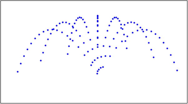
Figure 12-2. Creating a particle emitter
Creating a smoke effect
Let us now use our particle emitter to create a smoke effect. This is easier than you might think; in fact, you’ve already done most of the work. The code in the modified file, smoke-effect.js, is essentially the same as that in particle-emitter.js, except for a few relatively small changes.
function Spark(radius,r,g,b,alpha,mass){
     if(typeof(radius)==='undefined') radius = 2;
     if(typeof(r)==='undefined') r = 255;
     if(typeof(g)==='undefined') g = 255;
     if(typeof(b)==='undefined') b = 255;
     if(typeof(alpha)==='undefined') alpha = 1;
     if(typeof(mass)==='undefined') mass = 1;
     this.radius = radius;
     this.r = r;
     this.g = g;
     this.b = b;
     this.alpha = alpha;
     this.mass = mass;
     this.x = 0;
     this.y = 0;
     this.vx = 0;
     this.vy = 0;
}

Spark.prototype = {
     get pos2D (){
          return new Vector2D(this.x,this.y);
     },
     set pos2D (pos){
          this.x = pos.x;
          this.y = pos.y;
     },
     get velo2D (){
          return new Vector2D(this.vx,this.vy);
     },
     set velo2D (velo){
          this.vx = velo.x;
          this.vy = velo.y;
     },
     draw: function (context) {
          context.fillStyle = "rgba("+ this.r +","+ this.g +","+ this.b +","+ this.alpha +")";
          context.beginPath();
          context.arc(this.x, this.y, this.radius, 0, 2*Math.PI, true);
          context.closePath();
          context.fill();
     }
}
The first modification might appear a bit weird: we are giving the gravity constant g a negative value (–5)! What’s going on here? The thing is that smoke will tend to rise rather than fall because forces such as buoyancy (upthrust) will overcome the force of gravity. But instead of modeling buoyancy, it is simpler to modify gravity so that it acts upward because we are interested only in reproducing the visual effect of smoke approximately.
The second modification is that we are using a new object Spark, created especially for the next few animations. The Spark object looks similar to Ball in many respects, but it does away with extra properties like charge and gradient, which will not be needed here. More importantly, it introduces four new properties r, g, b, and alpha to replace the single property color of Ball. Spark also has a radius and a mass property.
The r, g, b, and alpha values are fed into the constructor (together with radius and mass) and have default values of 255, 255, 255 and 1 respectively. They are used in the draw() function to set the fillStyle when drawing a filled circle of the specified radius, with alpha representing transparency and r, g, b representing color in the RGB format. We specify the individual color and alpha channels separately so that we can manipulate them independently to produce visual effects (as you’ll see over the next several examples).
Armed with the new object Spark, we then modify the createNewParticles() method by creating new particles as instances of Spark rather than Ball, giving them radiuses between the values of 1 and 4 pixels. Modified lines are indicated in bold in the following code snippets.
function createNewParticles(ppos){
     var newParticle = new Spark(1+3*Math.random(),255,255,255,1,m);
     setPosVelo(newParticle,ppos);
     particles.push(newParticle);
}
The next modification is to introduce a new method, modifyObject(), which is called from within the for loop in move() and is therefore executed for each particle at each timestep.
function move(){
     context.clearRect(0, 0, canvas.width, canvas.height);
     if (particles.length < maxParticles){
          createNewParticles(posEmitter);
     }else{
          recycleParticles(posEmitter);
     }
     for (var i=0; i<particles.length; i++){
          var particle = particles[i];
          modifyObject(particle);
          moveObject(particle);
          calcForce(particle);
          updateAccel();
          updateVelo(particle);
     }
}
The modifyObject() method looks like this:
function modifyObject(obj){
     obj.radius *= 1.01;
     obj.alpha += -0.01;
}
All we are doing here is increasing the size of each particle by a constant factor and reducing its transparency by a fixed amount at each timestep.
The result of the previous additions and modifications is that the particles grow and fade as they rise, before disappearing altogether and being recycled. There is one more change that must be made to ensure that the recycling works properly. Because we have been modifying the radius and transparency of the particles, we need to reset those properties to their initial values when they are recycled. This is done by introducing a new method, resetObject() into the recycleParticles() method:
function recycleParticles(ppos){
     var firstParticle = particles[0];
     resetObject(firstParticle);
     setPosVelo(firstParticle,ppos);
     particles.shift();
     particles.push(firstParticle);
}
 function resetObject(obj){
     obj.radius = 1+3*Math.random();
     obj.alpha = 1;
}
If you were to run the code as shown here, you would get an interesting effect, but you couldn’t really call it smoke—see Figure 12-3.

Figure 12-3. An interesting effect, but not quite smoke yet!
Time to introduce filters! If you are not familiar with image filters, we encourage you to spend some time reading about them (you can find many tutorials on the Web) and playing around with them. The particular filter we want to use is the blur filter, which gives the edges of an image or HTML element a blurred appearance. There are several ways to achieve this. Since our interest here is on the physics rather than on filters per se, we’ll make do with what is probably the simplest approach: using CSS filters. Unfortunately the specification for this technology has not yet stabilized, so browser support is rather patchy at the time of writing. The following line added to the CSS file works in Chrome (and reportedly in Safari, too):
-webkit-filter: blur(3px);
This can also be set in the JavaScript file:
canvas.style.webkitFilter = "blur(3px)";
You can obviously change the degree of blurring by changing the number of pixels in the parentheses. Feel free to experiment with different values.
If you now run the code, you will see something that looks much more like smoke, as shown on screen in Figure 12-4.
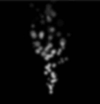
Figure 12-4. The smoke effect at last
This is a basic smoke effect that can be tweaked and enhanced in endless ways. Think of it as a starting point for further experimentation rather than as a final result. Moreover, there are lots of other ways to produce a smoke effect like this. The preceding method has been adapted from a tutorial in ActionScript by Seb Lee-Delisle that appeared in Computer Arts magazine (March 2008). It’s nice because of its simplicity and the fact that it can be done with pure code alone.
It is extremely easy to modify the smoke animation to produce something that looks like fire. The main changes are linked to the appearance of the particles; first we make them slightly bigger and orangey by modifying the first line in createNewParticles() to the following:
var newParticle = new Spark(3+3*Math.random(),255,100,0,1,m);
This makes particles with radiuses between 3 and 6 pixels. Subsequently, the particles are modified slightly differently than in the smoke simulation in modifyObject():
function modifyObject(obj){
     obj.radius *= 1.01;
     obj.alpha += -0.04;
     obj.g = Math.floor(100+Math.random()*150);
}
We now change the green color channel at every timestep to range between 100 and 250. We also increase the amount by which the alpha channel is incremented. Naturally, we need to modify the resetObject() method to restore the initial color and radius:
function resetObject(obj){
     obj.radius = 3+3*Math.random();
     obj.r = 255;
     obj.g = 100;
     obj.b = 0;
     obj.alpha = 1;
}
We have also tweaked the values of g and k, changing them to –2 and 0.003 respectively. Feel free to experiment by changing these parameter values. You might also look at the effect of changing the frame rate—perhaps changing fps dynamically, for example randomizing it or making it respond to user events.
The final change we made is to increase the brightness by modifying the canvas style using the following line of code in line 3 of the file:
canvas.style.webkitFilter = "blur(3px) brightness(2)";
If you run the code now you’ll see something like Figure 12-5. Of course, you need to see the actual animation to appreciate the effect and colors.

Figure 12-5. Creating a fire effect
Now that you have the basic tools at your fingertips, you can create more elaborate effects by applying the methods to different setups and by combining different techniques. For example, by attaching emitters to objects, you can create the illusion of the objects being on fire. You can also add wind, combine smoke with the fire, add sparks, and so on. Talking of sparks, let’s create some now.
The end result we want to achieve in this section is an animation that looks like fireworks: a series of little explosions, each generating colorful sparks that fall under gravity with drag. In order to get there, we will first add a couple of properties to our Spark instances and then create a sparks animation before finally adding extra features to make the fireworks.
Adding lifetime and age properties to sparks
Something like a spark exists for only a certain duration, after which it will need to be removed or recycled. It makes sense therefore to introduce a couple of new properties to represent the lifetime and age of a Spark instance. We have a choice of either adding the properties to the Spark object itself or adding them to instances of Spark. We choose the latter for the next couple of examples.
As you will recall from Chapter 2, it’s easy to add properties to object instances, as follows:
var spark = new Spark();
spark.lifetime = 10;
spark.age = 0;
This creates the two properties, lifetime and age, and assigns them values of 10 and 0, respectively. These represent the lifetime and age of spark in seconds. In subsequent code, you can then update its age as time progresses and to check and take the appropriate action if its age exceeds its lifetime.
Making sparks
Let us now apply the newly created lifetime and age properties to create sparks that exist for a specified duration. The code is in a file called sparks.js. We now have 200 particles and give them values of g, k, vx, and vy of 10, 0.005, 100, and –100, respectively (which you can change if you want). We have also changed the value of fps to 60 and specified a blur value of 1px and brightness factor of 2 in the corresponding CSS file. The methods that contain changes from the previous example (fire-effect.js) are reproduced here, with the modified lines highlighted in bold:
function move(){
     context.clearRect(0, 0, canvas.width, canvas.height);
     if (particles.length < maxParticles){
          createNewParticles(posEmitter);
     }else{
          recycleParticles(posEmitter);
     }
     for (var i=0; i<particles.length; i++){
          var particle = particles[i];
          modifyObject(particle,i);
          moveObject(particle);
          calcForce(particle);
          updateAccel();
          updateVelo(particle);
     }
}
function createNewParticles(ppos){
     var newParticle = new Spark(2,255,255,0,1,m);
     setProperties(newParticle,ppos);
     particles.push(newParticle);
}
function recycleParticles(ppos){
     var firstParticle = particles[0];
     resetObject(firstParticle);
     setProperties(firstParticle,ppos);
     particles.shift();
     particles.push(firstParticle);
}
function setProperties(obj,ppos){
     obj.pos2D = ppos;
     obj.velo2D = new Vector2D((Math.random()-0.5)*vx,(Math.random()-0.5)*vy);
     obj.lifetime = 6 + 2*Math.random();
     obj.age = 0;
}
function resetObject(obj){
     obj.alpha = 1;
}
function modifyObject(obj,i){
     obj.alpha += -0.01;
     obj.age += dt;
     if (obj.age > obj.lifetime){
          removeObject(i);
     }
}
function removeObject(num){
     particles.splice(num,1);
}
In createNewParticles(), each particle is given the same radius of 2 pixels and a yellowish color. The setPosVelo() method has been replaced by a setProperties() method that now does a bit more—it sets the lifetime and age of each particle in addition to its position and velocity. Because sparks can fly in any direction, each particle is given a random velocity in any direction. Then its lifetime is set to a random value between six and eight seconds. Its age is then initialized to zero.
The resetObject() method only needs to reset the transparency of each recycled particle to 1, since other properties (radius and color) are not changed during the animation.
The modifyObject() method decrements the alpha value of each spark as before, but additionally updates its age every timestep. The particle’s age is then checked against its lifetime: if it exceeds the lifetime, the removeParticle() method is called, which removes the particle from the particles array.
Run the simulation and you’ll see some nice sparks following the mouse (see Figure 12-6).

Figure 12-6. Making sparks
Making the fireworks animation
Now that we have sparks, we can use them to produce fireworks. Instead of producing the sparks continuously, we want to do that in a series of little explosions. We’ll have an initial explosion that will create a bunch of sparks with random velocities; these sparks will then fall under gravity with drag, fading with time. When each spark reaches the end of its lifetime, it will explode, producing further sparks. Obviously, we want to stop this process at some point. The easiest way to do that is to limit the duration of the animation by imposing a global cutoff time.
Following is the source code in the file fireworks.js in full, with modified parts highlighted in bold. Note that some code has also been removed compared to the previous sparks example, including the event listener/handler code.
var canvas = document.getElementById('canvas'),
var context = canvas.getContext('2d'),

var particles;
var m = 1;
var g = 10;
var k = 0.005;
var vx = 150;
var vy = -100;
var numSparks = 10;
var minLife = 2;
var maxLife = 4;
var duration = 6;
var fps = 30;
var t0, t, dt;
var acc, force;
var posEmitter;

window.onload = init;

function init() {
     particles = new Array();
     posEmitter = new Vector2D(0.5*canvas.width,200);
     createNewParticles(posEmitter,255,255,0);
     t0 = new Date().getTime();
     t = 0;
     animFrame();
}
function animFrame(){
     setTimeout(function() {
          animId = requestAnimationFrame(animFrame,canvas);
          onTimer();
    }, 1000/fps);
}
function onTimer(){
     var t1 = new Date().getTime();
     dt = 0.001*(t1-t0);
     t0 = t1;
     if (dt>0.2) {dt=0;};
     t += dt;
     move();
}
function move(){
     context.clearRect(0, 0, canvas.width, canvas.height);
     for (var i=0; i<particles.length; i++){
          var particle = particles[i];
          modifyObject(particle,i);
          moveObject(particle);
          calcForce(particle);
          updateAccel();
          updateVelo(particle);
     }
}
function createNewParticles(ppos,r,g,b){
     for (var i=0; i<numSparks; i++){
          var newParticle = new Spark(2,r,g,b,1,m);
          setProperties(newParticle,ppos);
          particles.push(newParticle);
     }
}
function setProperties(obj,ppos){
     obj.pos2D = ppos;
     obj.velo2D = new Vector2D((Math.random()-0.5)*vx,(Math.random()-0.5)*vy);
     obj.lifetime = minLife + (maxLife-minLife)*Math.random();
     obj.age = 0;
}
function modifyObject(obj,i){
     obj.alpha += -0.01;
     obj.age += dt;
     if (obj.age > obj.lifetime){
          if (t < duration){
               explode(obj);
          }
          removeObject(i);
     }
}
function explode(obj){
     createNewParticles(obj.pos2D,0,255,0);
}
function removeObject(num){
     particles.splice(num,1);
}
function moveObject(obj){
     obj.pos2D = obj.pos2D.addScaled(obj.velo2D,dt);
     obj.draw(context);
}
function calcForce(obj){
     var gravity = Forces.constantGravity(m,g);
     var drag = Forces.drag(k,obj.velo2D);
     force = Forces.add([gravity, drag]);
}
function updateAccel(){
     acc = force.multiply(1/m);
}
function updateVelo(obj){
     obj.velo2D = obj.velo2D.addScaled(acc,dt);
}
First note that we’ve changed the value of vx from 100 to 150. This is just so that the sparks spread horizontally more than vertically. We have also added four new variables: numSparks, minLife, maxLife, and duration to store the number of sparks, their minimum and maximum lifetimes, and the duration of the animation, respectively. The next change is that the createNewParticles() method is now called from within the init() method, not from within moveObject(). This means that the particles are created initially, not at every timestep. The createNewParticles() method is modified to accept new arguments that specify the RGB color of the sparks, to create a number numSparks of particles at each timestep instead of just one, and to assign to those particles the specified RGB color. The setProperties() method called from createNewParticles() then assigns each particle a random lifetime between minLife and maxLife.
The modifyObject() method is modified so that, as long as duration has not been exceeded, any particle that exceeds its lifetime explodes before being removed. The explosion is handled by the explode() method, which simply calls the createNewParticles() method and specifies the position of the dying particle as the location for the explosion and gives a new color for the next generation of sparks.
Run the code and you will be treated to a fireworks display (see Figure 12-7). Needless to say, you can tweak the animation endlessly to improve the appearance and add further effects such as trailing sparks, smoke, and even sound effects. We’ve done our job of showing you how to implement the basic physics. Now go for it!

Figure 12-7. Fireworks!
In the source code, we have also included a modified version of the simulation in a file named fireworks2.js. This is an interactive version where you click and hold down the mouse anywhere on the canvas. The number of sparks numSparks will be set to equal to twice the duration in seconds for which you hold down the mouse, so the longer you press the mouse the greater the number of sparks that will be produced per explosion. When you release the mouse, the initial explosion will take place at the location of the mouse. The colors of the sparks are also randomized in this version. Try it out!
Particle animations with long-range forces
It’s now time to transcend reality and start playing around with particles and physics. In this section, we’ll be moving lots of particles around under the action of long-range forces to create some interesting patterns and animations.
In this section and the next, we’ll generally be dealing with large numbers of particles and lots of calculations. To reduce any unnecessary overheads, we shall therefore make use of a slightly lighter version of the Ball object that we’ll call Star. The Star object is similar to the Ball object, but it does not draw a gradient fill and so does away with the extra code needed to do that. It also dispenses with the charge, gradient and angVelo properties. The remaining examples in this chapter will make use of the Star object.
Particle paths in a force field
Particle trajectories are commonly used in generative art projects. We’ll now set up a simple example using multiple particles that can be used as a basis for further explorations.
The idea of this animation is very simple, and it is similar in principle to the gravity field example in Chapter 10. We set up a number of stars randomly around a central attractor and give them small random velocities. The stars are subjected to a gravitational force toward the attractor and move around it, tracing trajectories.
The source file is called long-range.js and contains the following code:
var canvas = document.getElementById('canvas'),
var context = canvas.getContext('2d'),
var canvas_bg = document.getElementById('canvas_bg'),
var context_bg = canvas_bg.getContext('2d'),

var G = 10;
var attractors;
var orbiters;
var t0;
var dt;
var force;
var acc;
var numOrbiters = 20;
var numAttractors = 5;
var graph;

window.onload = init;

function init() {
     // create attractors
     attractors = new Array();
     for (var i=0; i<numAttractors; i++){
          var attractor = new Ball(20,'#333333',10000,0,false);
          attractor.pos2D = new Vector2D(Math.random()*canvas.width,Math.random()*canvas.height);
          attractor.draw(context_bg);
          attractors.push(attractor);
     }
     // create orbiters
     orbiters = new Array();
     for (var i=0; i<numOrbiters; i++){
          var orbiter = new Star(5,'ffff00',1);
          orbiter.pos2D = new Vector2D(Math.random()*canvas.width,Math.random()*canvas.height);
          orbiter.velo2D = new Vector2D((Math.random()-0.5)*50,(Math.random()-0.5)*50);
          orbiter.draw(context);
          orbiters.push(orbiter);
     }
     setupGraph();
     t0 = new Date().getTime();
     animFrame();
}

function animFrame(){
     requestAnimationFrame(animFrame,canvas);
     onTimer();
}
function onTimer(){
     var t1 = new Date().getTime();
     dt = 0.001*(t1-t0);
     t0 = t1;
     if (dt>0.2) {dt=0;};
     move();
}
function move(){
     context.clearRect(0, 0, canvas.width, canvas.height);
     for (var i=0; i<numOrbiters; i++){
          var orbiter = orbiters[i];
          plotGraph(orbiter);
          moveObject(orbiter);
          calcForce(orbiter);
          updateAccel(orbiter.mass);
          updateVelo(orbiter);
     }
}
function moveObject(obj){
     obj.pos2D = obj.pos2D.addScaled(obj.velo2D,dt);
     if (obj.x < 0 || obj.x > canvas.width || obj.y < 0 || obj.y > canvas.height){
          recycleOrbiter(obj);
     }
     obj.draw(context);
}
function updateAccel(mass){
     acc = force.multiply(1/mass);
}
function updateVelo(obj){
     obj.velo2D = obj.velo2D.addScaled(acc,dt);
}
function calcForce(obj){
     var gravity;
     force = Forces.zeroForce();
     for (var i=0; i<numAttractors; i++){
          var attractor = attractors[i];
          var dist = obj.pos2D.subtract(attractor.pos2D);
          if (dist.length() > attractor.radius+obj.radius){
               gravity = Forces.gravity(G,attractor.mass,obj.mass,dist);
               force = Forces.add([force, gravity]);
          }
     }
}
function recycleOrbiter(obj){
     obj.pos2D = new Vector2D(Math.random()*canvas.width,Math.random()*canvas.height);
     obj.velo2D = new Vector2D((Math.random()-0.5)*100,(Math.random()-0.5)*100);
}
function setupGraph(){
     graph = new Graph(context_bg,0,canvas.width,0,canvas.height,0,0,canvas.width,canvas.height);
}
function plotGraph(obj){
     graph.plot([obj.x], [-obj.y], '#cccccc', false, true);
}
There is little that you have not seen before in this code, and we’ll focus on the few new elements. In init() we create multiple attractors as Ball instances and multiple orbiters as Star instances. In calcForce(), we are subjecting each star to the gravitational force due to the attractors using the Forces.gravity() function, but note that if the star happens to be within a particular attractor we do not include the force that it exerts, effectively setting that force to zero. As in the gravity field example in Chapter 10, we use a graph object to plot the trajectory of each orbiter.
Run the simulation and play around by changing the parameters and modifying it in any way you can think of. For example, you could add a finite particle lifetime. If you have a slow machine, you might want to reduce the number of particles. You can come up with some interesting patterns (see, for example, Figure 12-8).
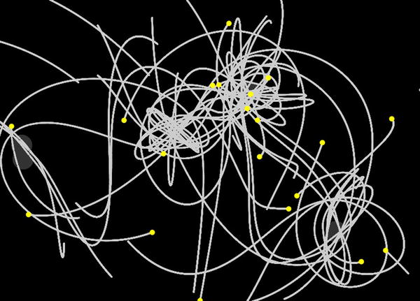
Figure 12-8. An example of particle trajectories under a central gravitational force
In this wacky example we are going to create something that does not reflect any real physics but is nevertheless interesting to watch!
A wormhole is a hypothetical object in which you enter a black hole and emerge at some other location in space. In our animation, we’ll have a wormhole made up of a black hole that sucks in stars and a white hole that spews them out again. To make the animation more visually interesting, the stars coming out of the black hole will be increased in size and given a randomized velocity back toward the black hole, creating a cycling system. What do you expect to happen eventually? Let’s find out. First we’ll show the simulation variables and parameter values and the init() function in the file wormhole.js:
var stars;
var numStars = 1000;
var massStar = 1;
var massAttractor = 10000;
var radiusAttractor = 20;
var posAttractor = new Vector2D(400,400);
var posEmitter = new Vector2D(400,100);
var G = 10;
var t0, dt;
var acc, force;

window.onload = init;

function init() {
     // create a stationary black hole
     var blackHole = new Star(radiusAttractor,'#222222',massAttractor);
     blackHole.pos2D = posAttractor;
     blackHole.draw(context_bg);
     // create a stationary white hole
     var whiteHole = new Star(10,'#ffffff'),
     whiteHole.pos2D = posEmitter;
     whiteHole.draw(context_bg);
     // create stars
     stars = new Array();
     for (var i=0; i<numStars; i++){
          var star = new Star(2,'#ffff00',massStar);
          star.pos2D = new Vector2D(Math.random()*canvas.width,Math.random()*canvas.height);
          star.velo2D = new Vector2D((Math.random()-0.5)*50,(Math.random()-0.5)*50);
          star.draw(context);
          stars.push(star);
     }
     t0 = new Date().getTime();
     animFrame();
}
We create a black hole and a white hole and place them some distance from each other, at locations denoted by posAttractor and posEmitter respectively. We next create 1000 stars and place them randomly on the canvas. The stars are animated as usual by calling animFrame(). The subsequent code is standard, the only new features cropping up in the calcForce() and recycleObject() methods:
function calcForce(obj){
     var dist = obj.pos2D.subtract(posAttractor);
     if (dist.length() < radiusAttractor){
          recycleObject(obj);
     }else{
          var gravity;
          force = Forces.zeroForce();
          if (dist.length() > radiusAttractor+obj.radius){
               gravity = Forces.gravity(G,massAttractor,massStar,dist);
               force = Forces.add([force, gravity]);
          }
     }
}
function recycleObject(obj){
     obj.pos2D = posEmitter;
     obj.velo2D = new Vector2D((Math.random()-0.5)*50,Math.random()*10);
     obj.radius *= 1.5;
}
The calcForce() method is nearly the same as in the previous example. The novelty is that we have a new recycleObject() method that is called if the star enters the black hole. The recycleObject() method instantly moves particles that enter the black hole to the location of the white hole, gives them a random downward velocity, and increases their radius by 50 percent.
If you run the code, you’ll find that the stars are sucked into the black hole, emerging larger out of the white hole. Because they are spewed around the black hole again, some of the stars are attracted back into it, while others end up in an orbit around it. Some stars might manage to escape, depending on the maximum magnitude of velocity you set. A few stars go through the wormhole a few times, growing bigger and bigger. Eventually you end up with stars of different sizes trapped in perpetual orbit around the black hole, as shown in Figure 12-9. Because those stars are in a closed orbit around the black hole and have originated from the white hole, their orbits close back on the white hole, giving the impression that the latter is also attracting them!
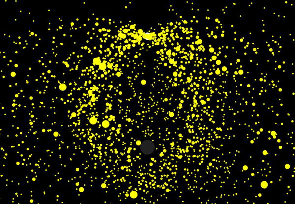
Figure 12-9. Stars circulating through a wormhole!
Interacting particle systems
So far, the particle systems we have looked at have not involved any mutual interactions between the particles. For example, you could let the particles exert a gravitational force on each other. This would create some interesting effects. The trouble is that the number of calculations then becomes very large as the number of particles is increased. For N particles, there are on the order of N2 interactions because every particle interacts with every other particle. Even with only 100 particles, that’s 10,000 extra gravity calculations per timestep! The next two examples illustrate different ways we may be able to handle this.
Multiple particles under mutual gravity
In this example, we will modify the gravity animations in the previous two examples by including mutual gravitational forces between the stars. In physics jargon, this will be a direct N-body calculation.
Again, let’s start by looking at the variable declaration/initialization and init() function in the relevant file, multigravity.js:
var stars;
var numStars = 200;
var massStar = 100;
var vmag = 10;
var massNucleus = 1;
var radiusNucleus = 20;
var posNucleus = new Vector2D(0.5*canvas.width,0.5*canvas.height);
var G = 1;
var eps = 1;
var rmin = 100;
var t0, dt;
var acc, force;

window.onload = init;

function init() {
     // create a stationary attracting nucleus
     var nucleus = new Star(radiusNucleus,'#333333',massNucleus);
     nucleus.pos2D = posNucleus;
     nucleus.draw(context_bg);
     // create stars
     stars = new Array();
     for (var i=0; i<numStars; i++){
          var star = new Star(2,'#ffff00',massStar*(Math.random()+0.1));
          star.pos2D = new Vector2D(Math.random()*canvas.width,Math.random()*canvas.height);
          star.velo2D = new Vector2D((Math.random()-0.5)*vmag,(Math.random()-0.5)*vmag);
          star.draw(context);
          stars.push(star);
     }
     t0 = new Date().getTime();
     animFrame();
}
Here we are creating a central attracting nucleus as well as 200 stars that are randomly positioned around it and have small random velocities. The mass of the nucleus is made 100 times larger than that of the stars, but those are parameters that you can change to see their effect. The only substantial difference from the previous examples is in the calcForce() method:
function calcForce(obj,num){
     var dist = obj.pos2D.subtract(posNucleus);
     var gravityCentral;
     if (dist.length() < radiusNucleus) {
          gravityCentral = new Vector2D(0,0);
     }else{
          gravityCentral = Forces.gravity(G,massNucleus,obj.mass,dist);
     }
     var gravityMutual = new Vector2D(0,0);
     for (var i=0; i<stars.length; i++){
          if (i != num){
               var star = stars[i];
               var distP = obj.pos2D.subtract(star.pos2D);
               if (distP.length() < rmin){
                    var gravityP = Forces.gravityModified(G,star.mass,obj.mass,distP,eps);
                    gravityMutual.incrementBy(gravityP);
               }
          }
     }
     force = Forces.add([gravityCentral, gravityMutual]);
}
You are already familiar with the first half of the code in calcForce(), which computes the force gravityCentral on the stars due to the central nucleus. The second half of the code calculates the total force gravityMutual on a star due to all the other stars (excluding itself, hence the if (i != pnum){} condition) and adds it to the gravityCentral force to get the total force on each star.
There are two new features in this code, in another if statement nested within the first:
if (distP.length() < rmin){
     var gravityP = Forces.gravityModified(G,star.mass,obj.mass,distP,eps);
     gravityMutual.incrementBy(gravityP);
}
The first new feature is the if condition, which checks to see whether the distance of the current star from any other star is less than a certain minimum distance rmin. The gravity force due to the latter star is included only if the condition is satisfied. This is called the local interaction approximation. The idea is that because gravity is an inverse square law, its magnitude falls off rapidly with distance. So if the other star is very far away, including the force it exerts won’t make much difference to the total force and is just a waste of resources. So you include only the influence of the nearest neighbors. In an accurate simulation, you would have to be careful to implement this approximation properly, as there are some subtleties. But because we are just playing around, so to speak, there is no need to go into those finer points. The value of rmin chosen in the code is 100 pixels, but you can experiment with other values. Giving rmin the value of 0 would effectively exclude all mutual interactions between the stars. Giving rmin a value larger than 800 would include interactions between all 200 stars: that’s about 400,000 extra gravity calculations per timestep, and will certainly slow down your animation!
The second new feature is that we are using a modified version of the gravity function called Forces.gravityModified() to compute the interactions between the stars. The new function is defined as follows:
Forces.gravityModified = function(G,m1,m2,r,eps){
     return r.multiply(-G*m1*m2/((r.lengthSquared()+eps*eps)*r.length()));
}
Comparing this with the Forces.gravity() function, you will find that we have introduced a new parameter eps, whose square is added to the r2 term in the denominator of the function. The corresponding mathematical formula is this:
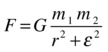
The ε symbol (the Greek letter epsilon) stands for the eps parameter. Why do we modify the gravity function in this way? When two objects exerting gravitational forces on each other get very close, the forces become very large or even infinite (because r goes to zero, and we end up dividing by a small number or zero). This, as you will recall from Chapter 6, causes the two objects to accelerate enormously and be sent flying off in random directions. The ε factor is a common “fudge” to bring that problem under control. Because ε2 is always positive (being the square of a real number), the denominator will never be zero. And as long as ε is small, it will not alter the force calculation much for most values of r except the very smallest. In the example, eps has a value of 1 pixel. You can also experiment with different values to see what effect it produces.
Run the simulation and experiment with different values of the parameters. For example, you can change the masses of the central nucleus and the stars to change the relative importance of the central force compared to the mutual forces between the stars. Running the code with the default values of the parameters will make the stars tend to lump together in different locations, with a few lingering around the central attractor. A screenshot is shown in Figure 12-10. Again, you may want to reduce the number of particles if the simulation runs slowly on your machine.

Figure 12-10. Lots of stars exerting gravitational forces on one another
A simple galaxy simulation
What would you need to do to simulate the motion of stars in a galaxy? Well, that is not a trivial job to do properly, typically requiring some serious hardware and lots of physics and code. But it is possible to cheat and come up with a very simplified approach. While the result certainly won’t look like that in more sophisticated approaches, it will give you something interesting to play and experiment with further.
The most obvious problem that we hit when attempting to model a system like this is how to handle the large number of particles you’d need. We are talking at least thousands here, and possibly tens of thousands. A direct N-body calculation is impractical with such large numbers of particles, especially for an animation that’s going to run in a web browser!
An alternative approach is to consider the motion of each star in the effective gravitational force field due to all the other stars taken together. This is the so-called mean field approach. The star system is then effectively considered as a non-interacting collisionless system with each star moving independently in that mean field. The mean field can of course evolve over time as the positions of the stars change, and this evolution needs to be incorporated in such a simulation.
There are numerical methods for calculating the mean field created by a general distribution of point masses, but they are beyond the scope of this book. However, if we make the assumption that the stars are distributed in a spherically symmetric way around the galactic center, the task becomes much simpler thanks to a neat mathematical principle. This principle says that for any spherically symmetric mass distribution, the gravitational force at any distance r from the center is the same force exerted by the total mass enclosed within a sphere of radius r, with that mass taken to be at the center. Any mass outside that radius does not have any effect. If you start a simulation with a spherically symmetric distribution of stars, it should remain spherically symmetric at all times. So you can apply this principle at each timestep.
The stars in a galaxy are not the only source of mass. Many galaxies have a central nucleus that may be a supermassive black hole. So the mass of this galactic nucleus needs to be taken into account. But that’s easy; we just use the Forces.gravity() function with a specified mass for the nucleus.
There is also something more exotic that lurks in galaxies: dark matter. In fact, it is estimated that most of the mass in a galaxy exists in a dark matter halo around the galaxy. Again, assuming spherical symmetry, the contribution of this dark matter to the gravitational force can be calculated in the same way as that of the stars.
With these basic ingredients, let’s put together a quick and dirty galaxy simulation. Much of the code in the relevant file galaxy.js looks similar to that in the previous examples, but we list the source code here in its full glory:
var canvas = document.getElementById('canvas'),
var context = canvas.getContext('2d'),

var stars;
var numStars = 5000;
var massStar = 10;
var veloMag = 20;
var maxRadius = 300;
var nucleus;
var massNucleus = 100000;
var radiusNucleus = 20;
var posNucleus = new Vector2D(0.5*canvas.width,0.5*canvas.height);
var G = 1;
var rmax = 500;
var constDark = 1000;
var A = 1;
var alpha = 0.5;
var t0, dt;
var acc, force;
var massStars = new Array(); // total mass of stars within radius r
var massDark = new Array();  // total mass of dark matter within radius r

window.onload = init;

function init() {
     // create a stationary attracting nucleus
     nucleus = new Star(radiusNucleus,'#333333',massNucleus);
     nucleus.pos2D = posNucleus;
     nucleus.draw(context);
     // initial distribution of stars
     stars = new Array();
     for (var i=0; i<numStars; i++){
          var star = new Star(1,'#ffff00',massStar);
          var radius = radiusNucleus + (maxRadius-radiusNucleus)*Math.random();
          var angle = 2*Math.PI*Math.random();
          star.pos2D = new Vector2D(radius*Math.cos(angle),radius*Math.sin(angle)).add(posNucleus);
          var rvec = posNucleus.subtract(star.pos2D);
          star.velo2D = rvec.perp(veloMag);
          star.draw(context);
          stars.push(star);
     }
     t0 = new Date().getTime();
     animFrame();
}

function animFrame(){
     requestAnimationFrame(animFrame,canvas);
     onTimer();
}
function onTimer(){
     var t1 = new Date().getTime();
     dt = 0.001*(t1-t0);
     t0 = t1;
     if (dt>0.2) {dt=0;};
     move();
}
function move(){
     context.clearRect(0, 0, canvas.width, canvas.height);
     nucleus.draw(context);
     calcMass();
     for (var i=0; i<numStars; i++){
          var star = stars[i];
          moveObject(star);
          calcForce(star,i);
          updateAccel(massStar);
          updateVelo(star);
     }
}
function moveObject(obj){
     obj.pos2D = obj.pos2D.addScaled(obj.velo2D,dt);
     obj.draw(context);
}
function updateAccel(mass){
     acc = force.multiply(1/mass);
}
function updateVelo(obj){
     obj.velo2D = obj.velo2D.addScaled(acc,dt);
}
function calcForce(obj){
     var dist = obj.pos2D.subtract(posNucleus);
     if (dist.length() < radiusNucleus) {
          force = new Vector2D(0,0);
     }else{
          force = Forces.gravity(G, massNucleus + massStars[Math.ceil(dist.length())] + massDark[Math.ceil(dist.length())], massStar, dist);
     }
}
function calcMass(){
     var distanceToCenter;
     var star;
     var massStarRing = new Array();
     var massDarkRing = new Array();
     for (var l=0; l<rmax; l++){
          massStarRing[l] = 0;
          massDarkRing[l] = constDark*l*l*Math.exp(-A*Math.pow(l,alpha));
     }
     for (var k=0; k<stars.length-1; k++){
          star = stars[k];
          distanceToCenter = star.pos2D.subtract(posNucleus).length();
          massStarRing[Math.ceil(distanceToCenter)] += star.mass;
     }
     massStars[0] = massStarRing[0];
     massDark[0] = massDarkRing[0];
     for(var j=1; j<stars.length-1; j++){
          massStars[j] = massStars[j-1] + massStarRing[j];
          massDark[j] = massDark[j-1] + massDarkRing[j];
     }
     //console.log(massNucleus,massStars[rmax-1],massDark[rmax-1]);
}
We first create a galactic nucleus of mass 100,000 units and radius 20 pixels and place it in the middle of the canvas. Then we create 5,000 stars (depending on your computer’s speed, you might want to reduce this number), each with mass 10 units, and place them in a random circular distribution around the galactic center (that’s what the lines of trigonometry code in init() achieve). Note that each “star” here really represents lots of stars; there are typically billions of stars in a galaxy, not thousands! The stars are then given an initial tangential velocity around the galactic center. The velocity magnitude for each star has the same value veloMag; that’s because observed galactic rotation curves show that the velocity in a galaxy is approximately independent of the distance from the galactic center. There are already a lot of parameters to play with here, such as the mass of the galactic center, the mass of each star, the rotational velocity, and so on. You can also try out different initial positions and velocities for the stars. In the file galaxy.js there are some commented lines with different options for these initial conditions. Try them out to see how they lead to different evolutions of the galaxy.
![]() Note If you have a slow machine, you may need to remove the line that contains the following code: if (dt>0.2) {dt=0;}. The large number of particles in this simulation means that a large number of calculations must be performed at each timestep, which could take longer than 0.2 seconds on a slow machine. In that case no movement whatsoever would take place!
Note If you have a slow machine, you may need to remove the line that contains the following code: if (dt>0.2) {dt=0;}. The large number of particles in this simulation means that a large number of calculations must be performed at each timestep, which could take longer than 0.2 seconds on a slow machine. In that case no movement whatsoever would take place!
Next let’s take a look at the calcForce() method. As you can see from the code, we are calculating the total gravitational force on each star at its distance from the center (dist) by using the Forces.gravity() function, with a mass that is the sum of the galactic nucleus mass and the masses of the stars and dark matter within that radius, as stored in the arrays massStars and massDark. These arrays are updated at each timestep by summing the mass at different distances from the center in the calcMass() method. A commented out line at the end of calcMass() outputs the three total masses to the console.
The mass of the stars is computed simply by locating the stars. For the dark matter, the situation is different because it is not included in the simulation as an object. Therefore, we prescribe a mass distribution based on the so-called Einasto profile, which is commonly used in computer simulations of dark matter. The mathematical form of that distribution is the following:
![]()
Here ρ0, A and α are constants that must be specified. This formula gives the mass density (mass per unit volume). To get the mass at a distance r, one must multiply this mass density by the volume of a thin spherical shell of thickness dr. This introduces an extra factor of 4πr2dr (surface area of sphere times the thickness of the spherical shell). This gives the formula that is coded in calcMass(). Don’t worry if this dark matter material seems a bit difficult to follow. We included it because it can change the dynamics of the interacting stars in a significant way, making for a “richer” simulation. But even if you don’t fully understand everything here, you can still play with the relevant parameters to explore the range of possible effects you can get with this additional physics included.
If you run the code with the default parameter values, you should find that after successive initial contractions and expansions, the star distribution settles into a quasi-steady state. Figure 12-11 shows a screenshot of what you might be able to see. One can even discern some structure in the form of rings at times, although it would take a more careful simulation to reproduce realistic physical structures properly. Again, you can change the parameters in galaxy.js, especially those of the dark matter distribution. It would be instructive to see how the simulation changes when you change the relative magnitudes of the galactic nucleus mass, the total star mass, and the total dark matter mass. Have fun!
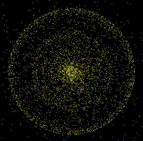
Figure 12-11. A simple galaxy simulation with 5000 particles
Summary
This chapter has provided a taste of what can be achieved with particles and some simple physics. In just a short chapter it is impossible to cover the subject fully. We therefore encourage you to search the Web and explore what has been achieved within the animation community and beyond. Many examples of inspiring creations by talented individuals exist, too numerous to mention here, but we’ve included relevant links on our web site: www.physicscodes.com.
You’ve had quite a lot of fun with particles in the last few chapters. In the next chapter we’ll look at how to model the motion of more complex extended objects.