![]()
Chapter 4 provided some of the general conceptual background for describing and analyzing motion. That background included a discussion of motion-related concepts such as velocity, acceleration, and force. In this chapter, we’ll use those concepts to formulate the physics laws that will allow you to calculate the motion of particles under any type of force. The next five chapters will then apply the laws to a number of different forces. We’ll illustrate the application of the principles with brief examples, with the aim of building on them in the next few chapters.
We have deliberately kept this chapter brief and focused on the fundamental laws and principles that you will need to apply to the examples in this part of the book and beyond. You can come back to this chapter as needed to refresh your understanding of the underlying physics principles, as you work your way through their applications in the rest of the book.
Topics covered in this chapter include the following:
- Newton’s laws of motion: Newton’s three laws provide the link between force and motion. These laws allow us to predict the motion of objects under the action of known forces.
- Applying Newton’s laws: We show you how to implement Newton’s laws of motion numerically in code and illustrate their use with a couple of examples.
- Newton’s second law as a differential equation: In physics textbooks, Newton’s second law is sometimes expressed as a differential equation and solved analytically using calculus. We briefly discuss the connection between that formulation and our numerical method, and illustrate it with an example.
- The principle of conservation of energy: We apply the principle of conservation of energy to motion by considering the potential and kinetic energy of moving particles.
- The principle of conservation of momentum: We take a look at conservation of momentum and its application to a simple example involving collisions.
- Laws governing rotational motion: We’ll note briefly that the preceding laws can be extended to objects undergoing rotational motion. We do not discuss rotation here, but will do so in later chapters.
Newton’s three laws of motion, formulated in his classic book Principia Mathematica in 1687, provide the link between force and motion. You might recall that we said in the previous chapter that the formula F = ma provides that link. This formula is actually the second of Newton’s three laws of motion. In fact, it is a special form of that law. In this chapter, we’ll go a bit deeper, looking at the general form of Newton’s second law as well as the two other laws.
Newton’s first law of motion (N1)
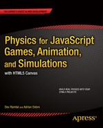
The first law of motion tells you what happens if there is no force acting on an object (see Figure 5-1). Think of an object that is at rest and not moving. If you don’t apply any force to it (in other words, if you leave it alone), what do you think will happen? That’s right—nothing. Things don’t suddenly start moving on their own. This is basically what the first law says. Common sense? But wait, there is more. Suppose the object is already moving and there is no force on it. What would happen to it? Everyday experience might tempt you into thinking that the object would slow down and finally stop. So you might be surprised to hear that the first law says that the object would carry on moving at its initial velocity as long as there is no force on it!
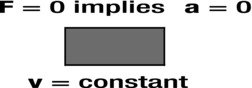
Figure 5-1. Schematic illustration of Newton’s first law of motion
This proposition seems to run somewhat counter to our everyday experience. For example, a ball rolling on the ground always comes to rest. In fact, it does so because friction with the ground is causing it to slow down. In the absence of friction, the ball would carry on indefinitely. This can be demonstrated by minimizing friction with the underlying surface—for example, by using marbles on a perfectly smooth horizontal surface. The marbles then move in a straight line for long distances without significant decrease in their velocity.
Another way of putting this is that you don’t need a force for an object to continue moving at constant velocity. You only need a force to make it change its velocity—for example, by starting to move, or speeding up or slowing down. In other words, you only need a force to make an object accelerate (or decelerate).
Armed with this insight, we can formulate Newton’s first law of motion succinctly in the following form, which covers both the cases of an object at rest and of one moving at constant velocity:
- N1: If the resultant force acting on an object is zero, its acceleration is zero. F = 0 implies a = 0.
This law is so important that we’ll say it in yet another way: If no resultant force acts on an object, its velocity must be constant (including zero). Conversely, if an object has a constant velocity (which may be zero), you know for certain that the resultant force on it must be zero.
Finally, note that we said that the resultant force is zero. We’re not saying that no forces are acting on the object. As you saw in Chapter 4, two or more forces acting on the same object can be in equilibrium so that their resultant is zero. In such a case, the first law will still hold. It does not distinguish between no resultant force and no force at all.
To put these concepts into context, the moveObject() method in the last two examples in Chapter 4 implements the first law; it takes a particle and moves it at its velocity forever. It knows nothing about forces.
Newton’s second law of motion (N2)
Newton’s second law of motion builds upon the first law (see Figure 5-2). The first law tells you what happens when no resultant force acts on an object. The second law tells you what happens when a resultant force does act on an object. It tells you that the object’s motion changes. But that’s not all. It tells you exactly by what amount it changes—it gives you an exact formula connecting the force applied and the change in motion produced.
![]()
Figure 5-2. Schematic illustration of Newton’s second law of motion
Recall from the last chapter that momentum (with the symbol p and defined as p = mv) represents the “quantity of motion” that an object possesses. Newton’s second law connects the force applied to the change in momentum it produces. We won’t go into how Newton arrived at that formula, but here it is:
- N2: If a resultant force F acts on an object, its momentum changes so that the rate of change of momentum is equal to the force applied:F = dp/dt.
This is the general form of Newton’s second law, and it may appear somewhat unintuitive, at least until you get used to it! In Calculus-speak, this tells us that the applied force is equal to the time derivative of momentum. Essentially, the time derivative of momentum tells us how fast the momentum is changing on an instantaneous basis. This means that the force being applied at any given time is equal to the change in momentum per unit time.
We have seen similar formulas before. For example, v = ds/dt and a = dv/dt. Newton’s second law is exactly of the same form: F = dp/dt. Note that the preceding equations for velocity and acceleration are actually definitions, whereas F = dp/dt is a law that tells us how things behave in the real world.
In this general form, the second law might seem quite different from the first law. In the first law, we were talking about acceleration, and now we are talking about rate of momentum change. There is actually a link between the two when we apply the second law to objects whose mass doesn’t change, such as particles.
To see the link, recall again that momentum is defined by p = mv. For a particle, the mass m is constant. In that case, the rules of calculus tell us that dp/dt = m dv/dt. If you’re into calculus, what we’ve done here is to calculate the (time) derivative of p, which must be equal to the derivative of mv (because these two things are equal: p = mv). But m is constant, so the derivative of mv is equal to m times the derivative of v. You probably recall that dv/dt = a (the definition of acceleration). Therefore, we conclude that for a particle, dp/dt = ma. Because Newton assures us that F = dp/dt, we’ve recovered our old friend F = ma. So here is the special form of Newton’s second law of motion:
- N2 (special): If a resultant force F acts on an object of constant mass m, it produces an acceleration a given by the formula F = ma.
If you now compare this form of the second law with the statement of the first law given in the last section, you’ll see that N1 is really just a special case of N2. Starting with F = ma and putting F = 0 gives ma = 0, and hence a = 0. In other words, F = 0 gives a = 0, which is exactly what the first law says. So the first law is “contained” within the second law. Good; that’s one fewer law to worry about!
You’ll use Newton’s second law in the form of F = ma most of the time. But bear in mind that it’s not the most general form of the law—it applies only if the mass m does not change. There is a third form of the law that applies when instead of an object of fixed mass m, you have a stream of substance moving at a certain velocity. For example, the exhaust gases from a rocket are pushed out at a constant velocity v relative to the rocket. Because v is now constant, calculus rules tell us that dp/dt = vdm/dt. Therefore, the force on the gases is given by F = vdm/dt, where dm/dt is the rate of change of mass (the mass of gas released per second). We’ll use this form of Newton’s second law to model a rocket in Chapter 6:
- N2 (alternate): The force F needed to move any substance at a rate of dm/dt at constant velocity v is given by F = vdm/dt.
Despite its simplicity, Newton’s second law is arguably the most important law in Newtonian mechanics. It’s almost magical how it connects forces and motion. But it is also utterly useless unless we know how to work out the forces acting on an object. We need force laws. We’ll look at some examples of force laws shortly. But before we do that, you want to know about Newton’s third law, don’t you?
Newton’s third law of motion (N3)
In the preceding chapter, we said that force is the cause of changes in motion. As you have just seen, Newton’s second law makes that statement much more precise, giving us a formula for calculating the change in motion arising from a given force. But so far, we haven’t said much about where forces come from. Many forces arise because of the presence of other objects. Newton’s first and second laws tell us how an object’s motion responds to an applied force. Newton’s third law tells us how two objects interact by exerting forces on each other. Here it goes:
- N3: If a body A exerts a force F on another body B, body B must in turn exert an equal and opposite force –F on body A.
What this means is that forces between objects always exist as an action-reaction pair. Both forces exist simultaneously; there is no delay between them. And even if their magnitudes and directions change with time, they remain equal and opposite at all times.
Newton’s third law of motion is frequently misunderstood and misquoted. One of the common mistakes is to think that action and reaction forces “balance” each other. In fact, in an action-reaction pair, the forces act on different objects. Therefore, it is wrong to think that they “balance” or “cancel” each other. In other words, they are not in equilibrium. Each force acts on a different object and affects its motion individually. Subtleties like these make Newton’s third law somewhat difficult to understand deeply at an abstract level. But it helps a lot to see how the law is applied in analyzing specific problems. For example, Newton’s third law is applied to analyze the interaction between two particles in the section “The principle of momentum conservation” that follows. You will also see it applied in the analysis of different examples throughout the book.
Here are some examples of action-reaction pairs of forces:
- Two colliding bodies exert equal and opposite forces on each other, even if they have different masses, as depicted in Figure 5-3.
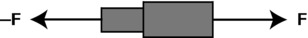
Figure 5-3. Schematic illustration of Newton’s third law of motion
- The Earth is exerting a force of gravity on you equal to your weight. This implies that you are also exerting an equal and opposite force of gravity on the Earth!
- In a rocket, the engine exerts a downward force on the exhaust gases, which in turn exerts an equal and opposite force on the rocket, propelling it forward.
Applying Newton’s laws
Practically the whole of the rest of this book is about applying Newton’s laws of motion. Here, we’ll just establish the method, create some force functions, and illustrate their application with some simple examples.
General method for applying F = ma
To analyze a problem for applying F = ma, use the following procedure:
- Draw a diagram representing the interacting objects in the problem.
- Choose the object whose motion is to be calculated and indicate using arrows all the forces acting on it due to other objects. Ignore the forces exerted by the object on other objects. This gives you a force diagram, as described in Chapter 4.
- Calculate the resultant force F on the object (using vector addition, as described in Chapter 3) and apply the second law F = ma to calculate the acceleration a.
In principle, that’s all there is to it. You have to do steps 1 and 2 using pen and paper. Let’s use JavaScript to help us do step 3.
Coding up motion under any force
What we need in order to achieve step 3 in the previous section is a general piece of code that allows you to calculate the forces on a particle, find their resultant, and hence compute their acceleration. You can then use the acceleration to update the velocity and position of the particle. Recall the sense in which we are using the term “particle,” as discussed in Chapter 4: any object whose inner structure is irrelevant from the point of view of the simulation. So, for our purposes, a particle could be a ball as well as a planet.
The general code structure for doing this will look very similar to the move() method in the example forces-example.js in the preceding chapter:
function move(){
     moveObject();
     calcForce();
     updateAccel();
     updateVelo();
}
As discussed, the moveObject() method simply moves the particle according to its existing velocity:
function moveObject(){
     particle.pos2D = particle.pos2D.addScaled(particle.velo2D,dt);
     context.clearRect(0, 0, canvas.width, canvas.height);
     particle.draw(context);
}
The rest of the code computes the force, works out the acceleration, and updates the velocity, ready to be used in the moveObject() method on the next timestep. The job of calcForce() is to calculate the resultant force on the particle. We’ll look at that last. The updateAccel() method updates the acceleration once we know the force. How do we do that? Of course, using F = ma to give a = F/m. So, with acc and force defined as Vector2D objects, updateAccel() is just a one-liner:
function updateAccel(){
     acc = force.multiply(1/particle.mass);
}
Recalling from Chapter 4 that Δv = aΔt, the updateVelo() method is just as simple:
function updateVelo(){
     particle.velo2D = particle.velo2D.addScaled(acc,dt);
}
Finally, the calcForce() method should calculate each force acting on the particle and then add them up to give their resultant, the force variable. The code that goes into calcForce() will depend on the problem and the forces involved. In the forces-example.js code in Chapter 4, calcForce() looked like this:
function calcForce(){
     force = new Vector2D(0,particle.mass*g-k*ball.vy);
}
In that simple example we just specified the force directly. But as our examples get more complicated, it will be useful to bunch together the different kinds of force laws we’ll come across into static methods in a single object that we’ll call Forces. To invoke the action of a particular force we can then do something like this:
function calcForce(){
     force = Forces.zeroForce();
}
All this method currently does is to set the force to zero. It does this using the Forces.zeroForce() method, which produces a Vector2D object with zero components. Of course, we haven’t said much about the Forces object yet, so let’s do that now.
The Forces object
Exactly what goes into calcForce()depends on the problem at hand, but it always involves specifying the forces on the particle and then adding them up. So, let’s build a new object to help us with these tasks.
The object we’ll build will basically just contain static methods for different types of forces. So we’ll name the object Forces, appropriately enough:
function Forces(){
}
In general, the force on a particle could depend on the particle properties (size, position, velocity, mass, charge), as well as on properties of the environment it is in, or on properties of other objects. These properties will need to be specified as arguments in the relevant methods.
Let’s look at some examples. First, let’s create a zero force. This is a force with a magnitude of zero, and therefore with components equal to zero.
Here is the static method that will make one:
Forces.zeroForce = function() {
     return (new Vector2D(0,0));
}
Next, let’s create a gravity force method:
Forces.constantGravity = function(m,g){
     return new Vector2D(0,m*g);
}
The force of gravity on an object of mass m is given by mg and points downward. Hence, we give the values of m and g as arguments and are given back a vector with the vertical (y) component being mg and the horizontal (x) component being zero. You’ll note that we’ve named the function constantGravity instead of simply gravity. This is because we are reserving the name gravity for the more general form of the force of gravity, which you’ll learn about in Chapter 6. The form of gravity given by mg is near-Earth gravity, as experienced by objects near the surface of the Earth. You’ll learn more about this in the next chapter.
As another example, let’s look at drag, which is the resistive force experienced by an object moving in a fluid such as air or water. We’ll take a much deeper look at drag in Chapter 7, but for now let’s just say that at low speeds the drag force is given by –kv. That’s a constant k times the velocity v of an object. The minus sign signifies that the drag force is in the opposite direction to the velocity. Let us create a function for this type of drag force, which we call linearDrag.
Here is the static method linearDrag:
Forces.linearDrag = function(k,vel){
     var force;
     var velMag = vel.length();
     if (velMag > 0) {
          force = vel.multiply(-k);
     }else {
          force = new Vector2D(0,0);
     }
     return force;
}
As you can see, the linearDrag function takes two arguments: the drag constant k (a Number) and the velocity vel (a Vector2D) of the object.
Next, we create a static method add() for adding any number of forces:
Forces.add = function(arr){
     var forceSum = new Vector2D(0,0);
     for (var i=0; i<arr.length; i++){
          var force = arr[i];
          forceSum.incrementBy(force);
     }
     return forceSum;
}
The add() method takes as argument an array of forces arr. It loops through the array, adding the forces in turn and returning the final vector sum. This is all we need for now. In the next few chapters, we’ll be adding many more force functions as static methods of the Forces object. To use the Forces object, don’t forget to add the file forces.js (available along with all the source code at http://apress.com) in your HTML file.
A simple example: projectile with drag
To demonstrate how to use the Forces class, let’s look at a simple example that brings together what we’ve been discussing in the previous two sections. Suppose we want a particle to move under gravity while experiencing the drag force (such as an object thrown or falling through a fluid such as air or water). The file forces-test.js shows how to do that:
var canvas = document.getElementById('canvas'),
var context = canvas.getContext('2d'),

var ball;
var t;
var t0;
var dt;
var animId;
var force;
var acc;
var g = 10;
var k = 0.1;
var animTime = 10; // duration of animation

window.onload = init;

function init() {
     ball = new Ball(15,'#0000ff',1,0,true);
     ball.pos2D = new Vector2D(50,400);
     ball.velo2D = new Vector2D(60,-60);
     ball.draw(context);
     t0 = new Date().getTime();
     t = 0;
     animFrame();
};
function animFrame(){
     animId = requestAnimationFrame(animFrame,canvas);
     onTimer();
}
function onTimer(){
     var t1 = new Date().getTime();
     dt = 0.001*(t1-t0);
     t0 = t1;
     if (dt>0.2) {dt=0;};
     t += dt;
     if (t < animTime){
          move();
     }else{
          stop();
     }
}
function move(){
     moveObject();
     calcForce();
     updateAccel();
     updateVelo();
}
function stop(){
     cancelAnimationFrame(animId);
}
function moveObject(){
     ball.pos2D = ball.pos2D.addScaled(ball.velo2D,dt);
     context.clearRect(0, 0, canvas.width, canvas.height);
     ball.draw(context);
}
function calcForce(){
     var gravity = Forces.constantGravity(ball.mass,g);
     var drag = Forces.linearDrag(k,ball.velo2D);
     force = Forces.add([gravity, drag]);
}
function updateAccel(){
     acc = force.multiply(1/ball.mass);
}
function updateVelo(){
     ball.velo2D = ball.velo2D.addScaled(acc,dt);
}
The new physics here takes place in the calcForce() method, where we include the forces of gravity and linear drag by making use of the relevant static methods of the Forces class. So we’ve invoked Forces.constantGravity(), using g = 10 and the particle mass. We’ve also invoked Forces.linearDrag() using k = 0.1. Then we added the two forces by passing them as an array argument to the Forces.add() method and assigned the result to the force variable.
Run the code and you will see a ball being thrown upward; it is then pulled down by gravity and slowed down by drag.
To appreciate the effect that the additional drag force has on the ball’s motion, replace the last two lines in calcForce() with the following line:
force = gravity;
This makes the ball move under gravity only. If you now run the code, you will see the ball following a parabolic trajectory, as in the projectile simulation in Chapter 4.
On the other hand, if you keep the drag force and increase the drag coefficient k to 0.5, the drag force will have a more extreme effect, quickly killing the horizontal motion of the ball and making it fall almost vertically thereafter—similar to what a balloon might do if you hit it upward.
This simple example demonstrates how easy it is to make use of the Forces object to build simulations, and how you can get different effects by changing the forces and their parameters in the calcForce() method.
Just to give you an idea of how flexible and powerful this approach is, let’s look at a somewhat more complicated example.
A more complicated example: floating ball
The example we are going to look at involves throwing a ball about in air or water and making it behave as it would do in real life. This example uses more physics than we’ve covered, so we won’t go into the details of the physics or coding involved, leaving a more complete discussion for Chapter 7. At this stage, we just want to whet your appetite by showing you what can be done with a fairly small amount of straightforward coding using the approach outlined in this section.
The source code for this example is in the file floating-ball.js. Before we look at this, a quick word on the HTML setup to give the desired visual environment as shown in Figure 5-4. As you can see from this screenshot, we have a rectangular area that represents water, and a ball which appears to be partially immersed in it. To achieve this visual effect, the water is drawn on a transparent canvas instance canvas_fg which is in the foreground, with the animation taking place on a different canvas instance named canvas. Take a look at the files floating-ball.html and style2.css to see how this is achieved.
Figure 5-4. The floating ball simulation
Here is the full code of floating-ball.js:
var canvas = document.getElementById('canvas'),
var context = canvas.getContext('2d'),
var canvas_fg = document.getElementById('canvas_fg'),
var context_fg = canvas_fg.getContext('2d'),

var ball;var t0;
var dt;
var animId;
var force;
var acc;
var g = 50;
var k = 0.01;
var rho = 1.5;
var V = 1;
var yLevel = 300;
var vfac = -0.8;

window.onload = init;
function init() {
     // create a ball
     ball = new Ball(40,'#0000ff',1,0,true);
     ball.pos2D = new Vector2D(50,50);
     ball.velo2D = new Vector2D(40,-20);
     //ball.velo2D = new Vector2D(20,-60);
     ball.draw(context);
     // create water
     context_fg.fillStyle = "rgba(0,255,255,0.5)";
     context_fg.fillRect(0,yLevel,canvas.width,canvas.height);
     // set up event listeners
     addEventListener('mousedown',onDown,false);
     addEventListener('mouseup',onUp,false);
     // initialize time and animate
     initAnim();
};

function onDown(evt) {
     ball.velo2D = new Vector2D(0,0);
     ball.pos2D = new Vector2D(evt.clientX,evt.clientY);
     moveObject();
     stop();
}

function onUp(evt) {
     ball.velo2D = new Vector2D(evt.clientX-ball.x,evt.clientY-ball.y);
     initAnim();
}
function initAnim(){
     t0 = new Date().getTime();
     animFrame();
}
function animFrame(){
     animId = requestAnimationFrame(animFrame,canvas);
     onTimer();
}
function onTimer(){
     var t1 = new Date().getTime();
     dt = 0.001*(t1-t0);
     t0 = t1;
     if (dt>0.2) {dt=0;};
     move();
}
function move(){
     moveObject();
     calcForce();
     updateAccel();
     updateVelo();
}
function stop(){
     cancelAnimationFrame(animId);
}

function moveObject(){
     ball.pos2D = ball.pos2D.addScaled(ball.velo2D,dt);
     context.clearRect(0, 0, canvas.width, canvas.height);
     ball.draw(context);
}
function calcForce(){
     //force = new Vector2D(0,ball.mass*g-k*ball.vy);
     var gravity = Forces.constantGravity(ball.mass,g);
     var rball = ball.radius;
     var xball = ball.x;
     var yball = ball.y;
     var dr = (yball-yLevel)/rball;
     var ratio; // volume fraction of object that is submerged
     if (dr <= -1){ // object completely out of water
          ratio = 0;
     }else if (dr < 1){ // object partially in water
          //ratio = 0.5 + 0.5*dr; // for cuboid
          ratio = 0.5 + 0.25*dr*(3-dr*dr); // for sphere
     }else{ // object completely in water
          ratio = 1;
     }
     var upthrust = new Vector2D(0,-rho*V*ratio*g);
     var drag = ball.velo2D.multiply(-ratio*k*ball.velo2D.length());
     force = Forces.add([gravity, upthrust, drag]);
     //force = Forces.add([gravity, upthrust]);
     if (xball < rball){
          ball.xpos = rball;
          ball.vx *= vfac;
     }
     if (xball > canvas.width - rball){
          ball.xpos = canvas.width - rball;
          ball.vx *= vfac;
     }
}
function updateAccel(){
     acc = force.multiply(1/ball.mass);
}
function updateVelo(){
     ball.velo2D = ball.velo2D.addScaled(acc,dt);
}
Without going into the details, you can see that we have a more complicated calcForce() method that includes three forces: gravity, upthrust, and drag. There is also some logic in calcForce() that tells the code how to work out the forces on the ball depending on where it is. Additionally, there is some logic to tell the code what to do at the boundaries. Finally, there are a number of parameters to do with the different forces. On the whole, though, this is certainly not an overly complex piece of code, and it should be possible for you to get the gist of what it’s doing.
The onDown() and onUp() methods allow the user to interact with the simulation by clicking the mouse. If you click anywhere on the canvas, the ball will immediately move there. If you hold down the mouse button, drag the cursor, and then release the mouse, the ball is imparted a velocity numerically equal to the distance between the ball and the point at which the mouse is released.
Run the simulation and play around to see how much it behaves like the real thing, all accomplished with a relatively small amount of code. It’s fun!
Newton’s second law as a differential equation
This section is especially meant for readers who want to understand the connection between what we are doing here and what you would typically find in physics textbooks or on physics web sites or Wikipedia. It provides a more in-depth understanding of the material but is not strictly required in the rest of the book. You can safely skip it if you wish.
If you are a serious physics programmer, it’s likely that you’ll find yourself digging into physics textbooks or online sources at some point or other, perhaps in search of some formula or to look for solutions to specific problems. Now, if you are looking for the solution of any problem involving Newton’s second law, chances are that you will come across differential equations, and pages of math to solve them analytically. How does all that math relate to our approach of solving Newton’s law numerically as discussed in the preceding section? In the next two subsections we explain the connection conceptually, and then illustrate it using a concrete example.
Taking a deeper look at F = ma
A differential equation contains derivatives of quantities. Solving differential equations is in general more complicated than solving ordinary algebraic equations because it involves integration (refer to Chapter 3).
Newton’s second law, in the form F = ma, might appear superficially like a simple algebraic equation.
However, it is useful to remember that acceleration is actually the derivative of velocity, a = dv/dt, so that we can also write Newton’s second law as

This is a so-called first-order differential equation with respect to velocity because it involves the first derivative of velocity. Recalling that v = ds/dt, we can then write the previous equation as

This is now a second-order differential equation with respect to displacement, because it involves the second derivative of displacement (refer to Chapter 3).
In general, the force F can be a function of position and velocity. You will see an example of such a force function shortly.
You will sometimes see Newton’s second law expressed in these forms if you look in physics textbooks. In principle, the preceding differential equations can be solved by integrating analytically or numerically to yield the displacement s and velocity v as a function of time. Most physics textbooks focus on analytical solutions. But an analytical solution is possible only in special cases and it requires application of calculus integration techniques. On the other hand, it is always possible to solve the differential equation numerically. In fact, this is what we are doing in the examples we have looked at. Specifically, we are integrating the first form of the differential equation in the updateVelo() method and then integrating the velocity to give the displacement in the moveObject() method.
The next example will illustrate a case in which we can solve Newton’s second law both analytically and numerically. We’ll use this example to show you what a typical analytical solution of this differential equation might look like. We’ll also compare the exact analytical solution with the numerically integrated solution to see how good the latter is.
Example: Falling under gravity and drag revisited
This example builds upon the one described in the previous chapter, in which we simulated the fall of a ball under the combined forces of gravity and drag, and showed that it attained terminal velocity as predicted by simple physics theory. Here we’ll update the example to compare the detailed analytical solution with the simulation.
The differential equation in this case is as follows (note that this is a 1D case; hence there is no need to use vector notation):
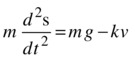
Or in first-order form in terms of velocity:
The analytical solution of this equation is given in many physics textbooks (for those interested, a derivation can be downloaded as supplementary material from www.physicscodes.com). For an object dropped from rest, it is this:
When the time t is large, the exponential term tends to zero (recall the review of the exponential function in Chapter 3). Therefore, according to this equation, v tends to a limiting value of mg/k, which is of course the terminal velocity. So the solution agrees with what we found in Chapter 4. In addition, it now tells us the velocity at any time t, not just the terminal velocity.
This solution can in turn be integrated to give the displacements at any time t. The result is this:

These analytical solutions for the displacement s and velocity v may now be compared with the simulated results. In forces-example2.js, we updated forces-example.js from Chapter 4 to make this comparison. We have also used the Forces methods in calcForce(); otherwise, the physics is identical to that in forces-example.js because the same forces (gravity and drag) are involved.
The relevant code is the function plotGraphs(), which plots graphs to compare the analytical and numerical values of s and v:
function plotGraphs(){
     graphDisp.plot([t], [ball.y-y0], '#ff0000'),
     graphDisp.plot([t], [m*g/k*(t+m/k*Math.exp(-k/m*t)-m/k)], '#0000ff'),
     graphVelo.plot([t], [ball.vy], '#ff0000'),
     graphVelo.plot([t], [m*g/k*(1-Math.exp(-k/m*t))], '#0000ff'),
}
In this code we are plotting the vertical displacement of the ball, which is ball.y minus its initial value y0, as well as its value as given by the analytical solution on the Graph instance graphDisp. Similarly, graphVelo displays the vertical velocity as computed by the code and the analytical solution. The simulation is shown in Figure 5-5. The agreement between the two is so good that the respective curves lie on top of each other in both graphs. So we’re happy that in this case the simple Euler integration scheme implemented in the code is actually doing a pretty decent job.
Figure 5-5. Comparing numerical and analytical solutions for a ball falling under gravity and drag
The principle of energy conservation
We introduced energy and its conservation in the previous chapter. The key point to reiterate here is that we can apply the principle of conservation of energy to work out how things move and how they interact with other things.
It’s also important to remember that the principle can apply to the conversion of energy between different forms, as well as to the transfer of energy between different objects. Here is a statement of the principle once more, in a slightly different form:
- Principle of Energy Conservation: In any conversion of energy between different forms, or in transfer of energy between different objects, the total amounts of energy before and after the conversion or transfer are always equal.
A particularly useful form of the principle is when the energy conversion or transfer involves only potential and kinetic energy. We refer to PE and KE collectively as mechanical energy.
Conservation of mechanical energy
Although the principle of conservation of energy in its general form is powerful and is always true, it may be difficult to apply in practice because it is not always easy to calculate all the energy forms involved in an interaction. For example, think of the energy transformations involved when a ball is dropped, falls through air, and bounces off a surface. The ball initially has PE and, as it falls through air, the PE is gradually converted into KE as it accelerates because of gravity. A small amount of energy is also converted into heat due to friction (drag) through the air. When it hits the surface, a large amount of energy may be transferred to the surface. Some more of the energy is usually converted into heat on impact, and some may be converted into sound as well. Now, we’ll steer clear of trying to calculate things like heat and sound energy because that can get pretty complicated. But sometimes, if they can be assumed to be small, we only need to deal with PE and KE In that case, we say that mechanical energy is conserved.
Conservation of mechanical energy is a particularly useful principle because it involves the energy forms associated with motion (KE) and position (PE). We’ll look at two examples of its application in this chapter. One is the elastic collision of two particles, when the total kinetic energy of the particles is conserved. We’ll look at this in the later section “The principle of momentum conservation.” The other example is the motion of a projectile (ignoring drag due to air resistance). Let’s look at this example now.
Example: Energy changes in a projectile
To simplify the example, let’s assume the projectile is launched vertically upward from ground level with some initial velocity u. Then we have a 1D problem with constant acceleration under gravity, and we can use the 1D version of the analytical equations of motion introduced in Chapter 4:
![]()

Here s = h, the height of the projectile above ground, and a = –g, where g is the acceleration due to gravity. So we can write this:
![]()
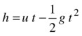
It is now straightforward to calculate the PE and KE of the projectile at any time by using the following:
![]()

Here is code that computes and plots the PE, KE, and their sum for 10 seconds, using values of m = 1, g = 10 px/s2, and u = 50 px/s. The source code is in projectile-energy.js.
var canvas = document.getElementById('canvas'),
var context = canvas.getContext('2d'),
var canvas_bg = document.getElementById('canvas_bg'),
var context_bg = canvas_bg.getContext('2d'),

var ball;

var animId;
var graph;
var m = 1;  // particle mass
var g = 10; // gravity
var u = 50; // initial velocity
var groundLevel = 350;
var n = 0;
var tA = new Array();
var hA = new Array();
var peA = new Array();
var keA = new Array();
var teA = new Array();

window.onload = init;

function init() {
     ball = new Ball(10,'#000000',m,0,true);
     ball.pos2D = new Vector2D(550,groundLevel);
     ball.draw(context);
     setupGraph();
     setupArrays();
     animFrame();
};
function setupGraph(){
     //graph = new Graph(context,xmin,xmax,ymin,ymax,xorig,yorig,xwidth,ywidth);
     graph = new Graph(context_bg,0,10,0,1500,50,350,450,300);
     graph.drawgrid(1,0.5,500,100);
     graph.drawaxes('t','p.e., k.e., total'),
}

function setupArrays(){
     var t;
     var v;
     for (var i=0; i<=100; i++){
          tA[i] = i*0.1;
          t = tA[i];
          v = u - g*t;
          hA[i] = u*t - 0.5*g*t*t;
          peA[i] = m*g*hA[i];
          keA[i] = 0.5*m*v*v;
          teA[i] = peA[i] + keA[i];
     }
}

function animFrame(){
     setTimeout(function() {
          animId = requestAnimationFrame(animFrame,canvas);
          animate();
     }, 1000/10);
}
function animate(){
     moveObject();
     plotGraphs();
     n++;
     if (n==hA.length){
          stop();
     }
}

function moveObject(){
     ball.y = groundLevel-hA[n];
     context.clearRect(0, 0, canvas.width, canvas.height);
     ball.draw(context);
}

function plotGraphs(){
     graph.plot([tA[n]], [peA[n]], '#ff0000', true, false);
     graph.plot([tA[n]], [keA[n]], '#0000ff', true, false);
     graph.plot([tA[n]], [teA[n]], '#000000', true, false);

function stop(){
     cancelAnimationFrame(animId);
}
The code should be easy to understand. Note that we have limited the frame rate to 10 fps by nesting the call to requestAnimationFrame() and animate() within a setTimeout() function. This slows the animation enough to enable the ball’s motion to be visually matched to the corresponding location on the plots. In Figure 5-6, we show the three plots as a function of time. The series of dots that curves upward is the PE, the series that curves downward is the KE, and the one that is horizontal (constant) is the total energy (the sum of PE and KE). From these plots, we learn that, when the projectile is initially launched at the ground, it has zero PE and maximum KE Then, for the first 5 seconds as it rises, its PE increases at the expense of its KE. At exactly 5 seconds, its KE is zero, signifying that it is momentarily at rest. This happens when it reaches its highest point. It then starts falling down again. As it does so, its PE starts falling again, and its KE increases as it speeds up toward the ground. Throughout its motion, the sum of the PE and KE is constant, as indicated by the horizontal series of dots. This demonstrates the conservation of energy. Note that the sum of PE and KE is only constant because we’ve omitted drag effects. If you include drag, then you’ll find that the sum of PE and KE decreases slightly with time. If you’re extra keen, you can show this by adding a drag term and integrating the equations of motion numerically to give v and h as a function of time.
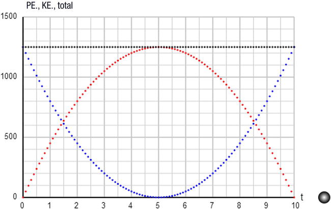
Figure 5-6. Energy graphs for a projectile—downward curve: KE; upward curve: PE; constant line: total
The principle of momentum conservation
As mentioned in the preceding chapter, there is a conservation principle for momentum just like the one for energy. Let’s state the principle first and then explain it:
- Principle of Momentum Conservation: For any system of interacting particles, the total momentum of all the particles remains constant, as long as no external forces act on the system.
“Interacting particles” means that the particles influence each other by exerting forces on each other. The forces can be of any type; for example, gravitational forces between stars in a galaxy. The principle is true regardless of the nature of the forces between the particles. Once you define your system, the particles in that system may be mutually subjected to any number of internal forces between themselves—the total momentum of that system will be conserved as long as there are no forces from external agents.
Conservation of momentum is closely connected with Newton’s laws of motion. In fact, under certain conditions, it may be derived from Newton’s laws. Let’s see how.
The starting point is Newton’s second law F = dp/dt, which we can write in the discrete form F = Δp/Δt. Multiplying both sides by Δt gives this:
![]()
This is, of course, just Newton’s second law written in a slightly different form, for a small but finite time interval Δt. What it tells us is that if a force F acts on a particle for a small duration Δt, multiplying F by Δt gives you the change in momentum Δp of the particle. We call the quantity FΔt the impulse due to the force. The preceding relationship is called the impulse-momentum theorem.
Next, imagine two particles interacting (exerting forces on each other; for example by colliding), as depicted in Figure 5-7. From Newton’s third law of motion, they exert equal and opposite forces simultaneously on each other. If they exert forces F and –F on each other for a time interval of Δt, they experience impulses of –F Δt and F Δt, respectively. From the impulse-momentum theorem, this implies that they exchange momentum, gaining –Δp and Δp, respectively. The total momentum of both particles is still the same, however, because one gains exactly the negative amount that the other gains; in other words, the momentum lost by one particle is gained by the other. This argument extends to any number of interacting particles, so we have the principle of conservation of momentum.
![]()
Figure 5-7. Two interacting particles exchanging momentum
Examples of momentum conservation include the following:
- An apple falling to Earth acquires downward momentum at each instant. Considering the apple-Earth system, the Earth itself must “fall” toward the apple to compensate. But because the mass of the Earth is so large, its velocity toward the apple is tiny.
- The exhaust gases from a rocket and the rocket itself get equal momentum changes in opposite directions.
- In an explosion, the total momentum of all the fragments must equal the momentum of the whole object before the explosion. If the object was initially at rest, the total momentum (as a vector sum of the momenta of all the fragments) after the explosion is still zero.
To give you a feel for how you’ll be applying this principle in practice, here is a numerical example. Suppose you fire a bullet of mass 40 g from a rifle of mass 1.6 kg, and the exit velocity of the bullet is 80 m/s. What is the recoil velocity of the rifle?
Let’s denote the mass and velocity of the bullet by m and v, respectively. And we’ll denote the mass and velocity of the rifle by M and V, respectively. Initially, both are at rest so that the total momentum is zero.
The principle of conservation of momentum therefore implies that the final momentum should be zero, too:
![]()
This equation can be easily rearranged to give this:

Substituting the values of m, v and M give the following:
![]()
Therefore, the recoil velocity of the rifle is –2 m/s. The minus sign means that it is in the opposite direction to the velocity of the bullet.
Example: 1D elastic collision between two particles
Conservation of momentum is especially useful in handling collisions between particles. A collision is a special type of interaction in which particles exert large forces on each other for a very brief duration.
The entirety of Chapter 11 is dedicated to collisions. Here we’ll look briefly at the simplest case of elastic collisions between two particles in 1D. Elastic in this context means that kinetic energy is conserved. In other words, no energy is converted to other forms (such as heat) during the collision. Momentum is, of course, always conserved.
Let’s say the masses of the particles are m1 and m2, their initial velocities before collision are u1 and u2, and their final velocities after collision are v1 and v2 (see Figure 5-8). Applying conservation of momentum then tells us that
![]()
Applying conservation of kinetic energy gives this:
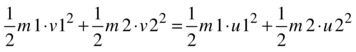
Remember that the formula for kinetic energy is 1/2 m v2.
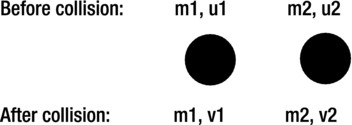
Figure 5-8. Change in particle velocities caused by a collision
What we have here are two equations containing two unknown quantities: the final velocities v1 and v2 of the two colliding particles. Everything else is known. These equations can be solved to give a general formula for v1 and v2 in terms of the known quantities m1, m2, u1, and u2. But we’ll save that for Chapter 11.
For now, let’s discuss the case where m1 = m2; that is, the two particles have the same mass. In that case, one can show that v1 = u2 and v2 = u1; in other words, the final velocity of particle 1 is equal to the initial velocity of particle 2, and vice versa. Particles of the same mass that collide elastically simply swap their velocities!
We’ll now build an example that implements this special case. The code is in collisions-test.js. Since it is a bit different from the other examples you’ve encountered so far, we reproduce the full code here before discussing it:
var canvas = document.getElementById('canvas'),
var context = canvas.getContext('2d'),
var t0;
var dt;
var animId;
var radius = 15; // ball radius
var balls = new Array();

window.onload = init;

function init() {
     makeBalls();
     t0 = new Date().getTime();
     animFrame();
};

function makeBalls(){
     setupBall('#0000ff',new Vector2D(50,200),new Vector2D(30,0));
     setupBall('#ff0000',new Vector2D(500,200),new Vector2D(-20,0));
     setupBall('#00ff00',new Vector2D(300,200),new Vector2D(10,0));
}
function setupBall(color,pos,velo){
     var ball = new Ball(radius,color,1,0,true);
     ball.pos2D = pos;
     ball.velo2D = velo;
     ball.draw(context);
     balls.push(ball);
}

function animFrame(){
     animId = requestAnimationFrame(animFrame,canvas);
     onTimer();
}
function onTimer(){
     var t1 = new Date().getTime();
     dt = 0.001*(t1-t0);
     t0 = t1;
     if (dt>0.2) {dt=0;};     checkCollision();
     move();
}
function move(){
     context.clearRect(0, 0, canvas.width, canvas.height);
     for (var i=0; i<balls.length; i++){
          var ball = balls[i];
          ball.pos2D = ball.pos2D.addScaled(ball.velo2D,dt);
          ball.draw(context);
     }
}
function checkCollision(){
     for (var i=0; i<balls.length; i++){
          var ball1 = balls[i];
          for (var j=i+1; j<balls.length; j++){
               var ball2 = balls[j];
               if (Vector2D.distance(ball1.pos2D,ball2.pos2D)<=ball1.radius+ball2.radius){
                    var vtemp = ball1.velo2D;
                    ball1.velo2D = ball2.velo2D;
                    ball2.velo2D = vtemp;
               }
          }
     }
}
Here we are creating and initializing three balls in the function makeBalls(), using a special function setupBalls() to minimize code repetition. To make things a bit more interesting, we create three balls aligned horizontally and give them different horizontal velocities. The animation loop code looks nothing out of the ordinary, but the onTimer() method that fires every timestep now contains an additional function checkCollision() in addition to the move() method.
In checkCollision(), we test for collisions between pairs of particles in the array. To do this, we use the Vector2D.distance(vec1,vec2) static method, which computes the distance between two points with position vectors vec1 and vec2. The logic of the collision detection algorithm is simple: if the distance between the centers of the two particles is less than or equal to the sum of their radii, it means they’ve collided. We then swap the velocities of the two particles.
As an aside, the Vector2D.distance() method computes the distance between two points by an appeal to the Pythagorean Theorem (see Chapter 3), as the following listing of relevant Vector2D methods shows:
Vector2D.prototype = {
     lengthSquared: function(){
          return this.x*this.x + this.y*this.y;
     },
     length: function(){
          return Math.sqrt(this.lengthSquared());
     },
}
Vector2D.distance =  function(vec1,vec2){
     return (vec1.subtract(vec2)).length();
}
If you run the code, you’ll see that, initially, all three balls get closer together. They then suffer three successive collisions that swap the velocities of each colliding pair. In the end, they all move away from each other.
Laws governing rotational motion
In this chapter, we have focused on translational motion, in which the object being considered changes its position. But what if an object rotates about a center or (if it’s an extended object) revolves on itself about some axis?
It turns out that analogous principles for rotational kinematics, dynamics, and conservation principles exist. For example, the analog of Newton’s laws of motion can be written down for rotational motion. Analogous to momentum, there is a quantity called angular momentum and it is also conserved.
We’ll look at rotational mechanics in Chapters 9 and 13.
Summary
This chapter laid the foundation for simulating the motion of particles under any type of force. The laws of motion and conservation principles discussed here can be applied in many different scenarios. In the remaining chapters in Part II, we’ll apply those laws to simulate the motion of objects under the action of a wide variety of force laws.