![]()
Long-Range Forces
In this last chapter of Part II, we’ll introduce yet more force laws. However, the approach and purpose here will be more playful than in previous chapters. You’ll learn concepts and techniques that you may not necessarily use for making realistic simulations, but more for producing fun animations and effects.
Topics covered in this chapter include the following:
- Particle interactions and force fields: There are two ways of viewing forces that act at a distance: in terms of direct interactions between particles, and in terms of force fields.
- Gravitational force: We revisit gravity as an example of a long-range force, giving further examples and building a black hole game!
- Electrostatic force: This is the force between electrically charged particles at rest, which can be attractive or repulsive. Interesting effects can be produced with electric forces.
- Electromagnetic force: Moving charges experience a magnetic force as well as an electric force. Together, they constitute an electromagnetic force, which can be used to produce more complicated types of motion.
- Other force laws: There is no reason you can’t invent your own force laws to produce cool effects. We’ll take a look at some examples, including so-called central forces of different types.
Particle interactions and force fields
Whenever we’ve talked about forces so far in this book, we’ve thought of them as being exerted by particles on other particles. But there is another way to think of forces that are exerted at a distance—we can think of them as being due to force fields. This is a fairly subtle concept, so we’ll take some time to explain it in the next couple of sections.
Interaction at a distance
In this chapter, we’ll deal exclusively with forces that are exerted and felt at a distance; the interacting objects don’t need to be in contact. Actually, at a fundamental level, all forces are like that, even contact forces. The difference is that contact forces are felt when two objects are very close together. Collisions are similar; they occur when two objects are so close together that their constituent molecules exert electric forces on each other. So the real distinction is between short-range and long-range forces. Contact forces and collisions involve short-range forces. Gravity is a long-range force. In general, both short-range and long-range forces can be attractive or repulsive.
From particle interactions to force fields
Historically, physicists were not very happy about the fact that forces like gravity appear to be exerted across empty space, with two remote objects being apparently able to influence each other instantly. This was the so-called action-at-a-distance problem. So they came up with the concept of a force field to replace the action-at-a-distance concept.
The idea of a force field, though seemingly esoteric, is actually quite simple. A field of force is simply a region of space where a force is felt. If you have two objects with mass, such as a star and a planet, the usual way to think of gravity is that they each exert a gravitational force on each other. In the field concept, you say that the star sets up a gravitational field that permeates the space around it. Any other object, such as a planet, then experiences a force due to the field at the point where it is located. The key idea is that the field mediates the interaction between the star and the planet. There is then no action-at-a-distance anymore; the force felt by the planet is a local one, due to the force field that exists locally. In fact, the force field exists whether or not there is a planet there to experience a force.
Note that in the previous example, the planet also sets up its own gravitational field, which then causes the star to experience a force equal and opposite to that experienced by the planet, in accordance with Newton’s third law of motion.
As we know, the force felt by the planet depends on its distance from the star. In the field concept, the variation of the force with distance is encapsulated in the concept of field strength. In the case of gravity, the field strength decreases with distance from the source of the field (in this case, a star). In the next section we’ll see the precise form of the field strength due to the star. It is also customary to refer to the field strength simply as the field.
Similar ideas apply to other long-range forces, such as electric forces. Particles create force fields. Other particles then experience forces in the presence of that field. The amount of force they experience depends on the field strength.
Why should you care about force fields? One important practical advantage is that force fields free us from the need to have particles just so they can exert forces. As you’ll see later in the chapter, we can produce a force field without worrying about how it can be produced by particles. This gives us great flexibility in the type of forces we can subject particles to. The concepts of force field and field strength are especially useful in connection with electric and magnetic forces, but let’s take a closer look at them in the context of gravity. They will then be easier to appreciate when we talk about the rather more abstract electric and magnetic fields.
Gravity is an archetypal example of a long-range force. The field strength in this case is defined as the force per unit mass that acts on a particle at any given point in the field. This is a sensible definition: It tells us how strong the gravity force field is by telling us the force that it exerts on an object of unit mass.
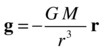
Gravitational field strength is a vector denoted by the symbol g. The definition tells us that

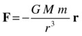
You will recognize this as being equivalent to the familiar formula for the gravitational force on an object of mass m:
![]()
So, the gravitational field strength is a vector with magnitude equal to the acceleration due to gravity g. In particular, that means it has the same value for all objects, regardless of their mass or other characteristics. In general, the gravitational field strength vector g can change with position, just like the (non-bolded) scalar g. In a uniform gravitational field, such as close to the surface of the Earth, both g and g are constant.
To reiterate an important point, the key thing with the definition of the gravitational field strength is that it is a property only of the field, as it exists independently of any object that may experience a force due to it. Whereas the gravitational force on an object will depend on its mass, the gravitational field strength g itself tells us the force per unit mass at any point in the field. From this, we can work out the force F on any mass m by multiplying by m.
Gravitational field due to a particle
The gravitational field strength due to a particle of mass M, such as a star, can be computed starting from Newton’s law of gravitation:
Here, m is the mass of any other particle in the field generated by the mass M, and r is its position vector relative to the source of the field.
Because the gravitational field strength is defined by g = F/m, we just have to divide the preceding formula by m to give this:
As you can see explicitly in the preceding formula, the gravitational field g depends only on the mass M of the particle that is producing it and the position vector from the particle, but not on any other particles that may be present. We can also deduce that the magnitude of g is given by g = GM/r 2, consistent with the variation of acceleration due to gravity derived in Chapter 6.
In general, g could be much more complicated than this simple formula. In a galaxy, for example, g is the vector sum of all the fields produced by the individual stars (all of which are, of course, moving). But simulating the motion of stars in a galaxy can be done much more efficiently using the field concept than by directly calculating all the forces between every pair of stars, as you’ll see in Chapter 12. Meanwhile, it’s time to start playing with some simpler examples of gravity as a long-range force.
Gravity with multiple orbiters
Our first example will involve a single gravitational attractor, which will be held fixed. We borrow the orbits simulation from Chapter 6, but we’ll add more orbiting planets to make it more interesting and to illustrate the fact that each planet experiences a different gravitational field strength at any given time, and therefore moves along a different trajectory. Here is the modified code that does this in orbits.js:
var canvas = document.getElementById('canvas'),
var context = canvas.getContext('2d'),
var canvas_bg = document.getElementById('canvas_bg'),
var context_bg = canvas_bg.getContext('2d'),

var M = 1000000; // sun's mass
var G = 1;
var sun;

var planets;
var t;
var t0;
var dt;
var force;
var acc;
var numPlanets = 3;

window.onload = init;

function init() {
     // create a stationary sun
     sun = new Ball(70,'#ff9900',M,0,true);
     sun.pos2D = new Vector2D(400,300);
     sun.draw(context_bg);
     // create planets
     planets = new Array();
     var radius = new Array(10,6,12);
     var mass = new Array(10,3,15);
     var color = new Array('#0000ff','#ff0000','#00ff00'),
     var pos = new Array(new Vector2D(400,50),new Vector2D(500,300),new Vector2D(200,300));
     var velo = new Array(new Vector2D(65,0),new Vector2D(0,100),new Vector2D(0,-70));
     for (var i=0; i<numPlanets; i++){
          var planet = new Ball(radius[i],color[i],mass[i],0,true);
          planet.pos2D = pos[i];
          planet.velo2D = velo[i];
          planet.draw(context);
          planets.push(planet);
     }
     t0 = new Date().getTime();
     t = 0;
     animFrame();
}
function animFrame(){
     requestAnimationFrame(animFrame,canvas);
     onTimer();
}
function onTimer(){
     dt = 0.001*(new Date().getTime() - t0);
     t0 = new Date().getTime();
     t += dt;
     move();
}
function move(){
     context.clearRect(0, 0, canvas.width, canvas.height);
     for (var i=0; i<numPlanets; i++){
          var planet = planets[i];
          moveObject(planet);
          calcForce(planet);
          updateAccel(planet.mass);
          updateVelo(planet);
     }
}
function moveObject(obj){
     obj.pos2D = obj.pos2D.addScaled(obj.velo2D,dt);
     obj.draw(context);
}
function updateAccel(mass){
     acc = force.multiply(1/mass);
}
function updateVelo(obj){
     obj.velo2D = obj.velo2D.addScaled(acc,dt);
}
function calcForce(planet){
     force = Forces.gravity(G,M,planet.mass,planet.pos2D.subtract(sun.pos2D));
}
The main point here is that we are creating three planets and then initializing their positions and velocities so that they end up orbiting the sun. The planets are placed at different distances from the sun and each is then given an initial tangential velocity. The magnitudes of the velocities are chosen essentially by trial and error; or you can use the method given in Chapter 9 to choose the velocities that will give a roughly circular orbit. Note that the move() function loops over each planet, applying the functions moveObject(), calcForce(), updateAccel() and updateVelo() to each in turn.
If you run the code, you’ll get a nice solar system toy simulation (see Figure 10-1). The basic physics is there. For example, the nearer a planet is to the sun, the faster it orbits. But this simulation is not completely accurate. As you saw in earlier examples, the Euler integration scheme quickly accumulates errors. If you are looking to do an accurate Solar System simulation, you’ll need a better integrator. We’ll do that in Chapter 16, where we’ll also account for the forces between the planets as well as input accurate data on the masses, sizes, positions, and velocities of the planets.
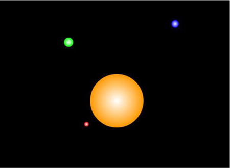
Figure 10-1. Multiple orbiting planets around a sun
Gravity with multiple attractors
Let’s complicate the previous simulation a little by adding another attractor. As in that example, we’ll keep the attractors fixed. It’s not difficult to make them move; that would produce some interesting overall motion. But we’d have to be more careful with our numerical integration scheme. We’ll come back to this issue in Chapter 14.
The new code is in a file called attractors.js and differs from orbits.js essentially in the init() and calcForce() methods. Let’s look at the former first:
var numOrbiters = 3;
var numAttractors = 2;

function init() {
     // create attractors
     attractors = new Array();
     var radiusA = new Array(20,20);
     var massA = new Array(1000000,1000000);
     var colorA = new Array('#ff9900','#ff9900'),
     var posA = new Array(new Vector2D(300,300),new Vector2D(500,300));
     for (var i=0; i<numAttractors; i++){
          var attractor = new Ball(radiusA[i],colorA[i],massA[i],0,true);
          attractor.pos2D = posA[i];
          attractor.draw(context_bg);
          attractors.push(attractor);
     }
     // create orbiters
     orbiters = new Array();
     var radius = new Array(8,8,8);
     var mass = new Array(1,1,1);
     var color = new Array('#0000ff','#ff0000','#00ff00'),
     var pos = new Array(new Vector2D(400,300),new Vector2D(400,400),new Vector2D(300,400));
     var velo = new Array(new Vector2D(0,60),new Vector2D(10,60),new Vector2D(90,0));
     for (var i=0; i<numOrbiters; i++){
          var orbiter = new Ball(radius[i],color[i],mass[i],0,true);
          orbiter.pos2D = pos[i];
          orbiter.velo2D = velo[i];
          orbiter.draw(context);
          orbiters.push(orbiter);
     }
     t0 = new Date().getTime();
     t = 0;
     animFrame();
}
The code is basically self-explanatory: We create two attractors and three orbiters, all as Ball instances. The attractors are given the same radius and mass. The initial position and velocity of the orbiters are then set. As we shall see, completely different trajectories result from those different initial conditions.
In calcForce() we calculate and then sum the forces acting on each orbiter due to all the attractors. The code can handle any number of attractors.
function calcForce(orbiter){
     var gravity;
     force = Forces.zeroForce();
     for (var i=0; i<numAttractors; i++){
          var attractor = attractors[i];
          gravity = Forces.gravity(G,attractor.mass,orbiter.mass,orbiter.pos2D.subtract(attractor.pos2D));
          force = Forces.add([force, gravity]);
     }
}
Run the code with the initial conditions for the three orbiters as specified in attractors.js. The blue orbiter has position vector (400,300) and velocity vector (0,60). This positions the orbiter exactly in the middle of the two attractors and gives it a downward velocity of 60 px/s. You’ll see that the orbiter oscillates up and down, so that it is at the same distance from each attractor.
The red orbiter has position vector (400,400) and velocity vector (10,60). You’ll find that this orbiter moves in an interesting way: orbiting each attractor alternately, but doing a twist in between so that it orbits both of them in a clockwise sense. If you now keep the same initial position but change the initial velocity to (120,0), you’ll see that the orbiter orbits both attractors. In general, you could have a distribution of different attractors and it would still be possible for an object to orbit the whole bunch.
The green orbiter has position vector (300,400) and velocity vector (90,0). This orbiter orbits each attractor alternately, but does so in the opposite sense by following a figure-eight trajectory.
Note that if you let the simulation run for long enough you might start seeing the orbits change due to numerical inaccuracies in the integration scheme. As discussed in the previous section, we will look at how to resolve this issue in Chapter 14.
The key lesson learned from these experiments (see Figure 10-2) is that although the gravitational field is fixed by the attractors, the actual trajectories of particles in that field will also depend on their positions and velocities.
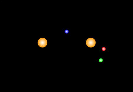
Figure 10-2. Orbiters moving under the gravitational influence of two attractors
Needless to say, there are many ways you can experiment with this simulation. As an exercise, why don’t you add another attractor and see what kind of motion you get?
Particle trajectories in a gravity field
In this next example, we have a number of attractors, giving rise to a complicated gravity field. The resulting trajectories of particles in such a field can be quite complex and sometimes difficult to predict. To make the example even more interesting, we assume that our attractors are black holes. We modify the attractors.js code from the previous example to implement these new features. Let us first take a look at the init() method:
function init() {
     // create attractors
     attractors = new Array();
     for (var i=0; i<numAttractors; i++){
          var r = 20*(Math.random()+0.5);
          var m = (0.5*c*c/G)*r;
          var attractor = new Ball(r,'#000000',m,0,false);
          attractor.pos2D = new Vector2D(Math.random()*canvas.width,Math.random()*canvas.height);
          attractor.draw(context_bg);
          attractors.push(attractor);
     }
     // create orbiters
     orbiters = new Array();
     var color = new Array('#0000ff','#ff0000','#00ff00'),
     for (var i=0; i<numOrbiters; i++){
          var orbiter = new Ball(5,color[i],1,0,true);
          orbiter.pos2D = new Vector2D(Math.random()*canvas.width,Math.random()*canvas.height);
          orbiter.velo2D = new Vector2D((Math.random()-0.5)*100,(Math.random()-0.5)*100);
          orbiter.draw(context);
          orbiters.push(orbiter);
     }
     setupGraph();
     t0 = new Date().getTime();
     t = 0;
     animFrame();
}
In this code, we create some black holes as ball instances, place them at random positions on the canvas, and put references to them in an array named attractors. We then create three orbiters, also as ball instances (colored blue, red and green as in the previous examples), and assign them a random position and a random velocity. As you can see from the code, to set the masses of the black holes we’ve used the formula M = (0.5c 2/G) R, where M is the mass and R is the radius of the black hole (which is given a random value between 10 and 30 pixels in the code). What is c, and where does this formula come from? This is the formula for the mass of a black hole in terms of its radius. The constant c is the speed of light. Our black holes are actually hypothetical Newtonian black holes; real (Einsteinian) black holes do not obey Newton’s law of gravitation, but require Einstein’s General Relativity (a much more complicated theory that we have no intention of simulating in this book!). The value of c will determine the range of masses of the black holes. It’s a case of playing with that value to make the black holes produce sufficient, but not too much, attraction so that the particles have a chance to do something interesting before being swallowed up by a black hole. The value we chose is 300.
The calcForce() method loops over all the attractors and sums their gravity forces as in the previous example. In addition, if the orbiter collides with any black hole it disappears and is “recycled” by calling the recycleOrbiter() method, as shown in the highlighted code within calcForce():
function calcForce(obj){
     var gravity;
     force = Forces.zeroForce();
     for (var i=0; i<numAttractors; i++){
          var attractor = attractors[i];
          var dist = obj.pos2D.subtract(attractor.pos2D);
          if (dist.length() > attractor.radius+obj.radius){
               gravity = Forces.gravity(G,attractor.mass,obj.mass,dist);
               force = Forces.add([force, gravity]);
          }else{
               recycleOrbiter(obj);
          }
     }
}
The recycleOrbiter() method simply reinitializes the position and velocity of the orbiter:
function recycleOrbiter(obj){
     obj.pos2D = new Vector2D(Math.random()*canvas.width,Math.random()*canvas.height);
     obj.velo2D = new Vector2D((Math.random()-0.5)*100,(Math.random()-0.5)*100);
}
The orbiter is also “recycled,” if it goes outside of the visible stage area, by a piece of if logic in the moveObject() method:
function moveObject(obj){
     obj.pos2D = obj.pos2D.addScaled(obj.velo2D,dt);
     if (obj.x < 0 || obj.x > canvas.width || obj.y < 0 || obj.y > canvas.height){
          recycleOrbiter(obj);
     }
     obj.draw(context);
}
You’ll notice that we also call a plotGraph() method in the move() method. What’s this about? Well, we are not really plotting a graph, but the trajectory of the orbiter. But we can do this using a Graph instance that has the same range as the stage. This is done in the setupGraph() method, which is called within the init() method. The plotGraph() method then plots the y position of the orbiter against its x position. Because plotGraph() is called within move(), it executes on each timestep, so the code effectively traces out the trajectory of the orbiter:
function setupGraph(){
     graph = new Graph(context_bg,0,canvas.width,0,canvas.height,0,0,canvas.width,canvas.height);
}
function plotGraph(obj){
     graph.plot([obj.x], [-obj.y], obj.color, false, true);
}
Take a look at the file gravity-field.js if you want to see how all this code fits together. Run the code, and you’ll be treated to some interesting trajectories as each orbiter moves through the complex gravity field and eventually ends up into a black hole. Each time this happens, it reappears somewhere else and traces out another trajectory that either ends into a black hole or just outside of the stage area. Figure 10-3 shows the type of result you’ll be able to see. The randomness in the initial conditions of the particles has the consequence that different patterns emerge over time, so you might want to leave the simulation running for some time to see this. Moreover, each time you run the simulation you will get a different configuration of black holes that will also give different patterns of particle trajectories.
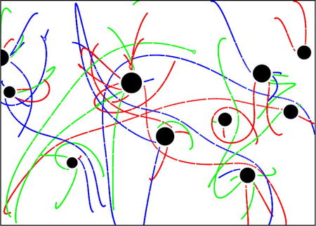
Figure 10-3. Particle trajectories in the gravity field of black holes
Building a simple black hole game
In this next project, we’ll be a bit more adventurous and actually build a simple game by modifying the preceding simulation. Figure 10-4 shows a screenshot of what the game will look like. The objective of the game is to navigate a spaceship (the triangle) through a black hole field. The spaceship starts off near the lower end of the stage, and you win if you can pass the winning line at the top. Each time you win, a new black hole is added. The positions of the black holes are initialized randomly so that their centers all lie between the winning line and another horizontal line lower down. You lose a life each time a black hole captures the spaceship. If you go off the stage, the spaceship is repositioned at its initial location.
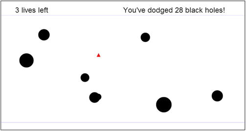
Figure 10-4. The black hole game
The bits of code that create the visual setup are invoked from the init() function in the file black-holes.js:
function init() {
     ship = new Rocket(12,12,'#ff0000',1);
     ship.pos2D = new Vector2D(0.5*canvas.width,canvas.height-50);
     ship.draw(context);
     attractors = new Array();
     addAttractor();
     setupText();
     setupScene();
     setupEventListeners();
     t0 = new Date().getTime();
     t = 0;
     animFrame();
}
First we create a spaceship named ship as an instance of the Rocket object, borrowed from Chapter 6. Next we create an array called attractors, and then call a function addAttractor() that creates our first black hole and puts a reference to it in the attractors array:
function addAttractor(){
     var r = 20*(Math.random()+0.5);
     var m = (0.5*c*c/G)*r;
     var attractor = new Ball(r,'#000000',m,0,false);
     attractors.push(attractor);
}
The code that creates the black holes and assigns their properties is similar to that in the previous example. In the code in black-holes.js we reduced the speed of light to 200 px/s so that the attraction is not too strong, making it actually possible to avoid the black holes!
Next in init(), the setupText() function is called. This function sets the text properties such as font size and family.
function setupText(){
     context_bg.font = "18pt Arial";
     context_bg.textAlign = "left";
     context_bg.textBaseline = "top";
}
Then the setupScene() method is called; it displays the visual elements on canvas_bg:
function setupScene(){
     context_bg.clearRect(0, 0, canvas_bg.width, canvas_bg.height);
     drawLines();
     showLives();
     showScore();
     for (var i=0; i<attractors.length; i++){
          var attractor = attractors[i];
          attractor.pos2D = new Vector2D(Math.random()*canvas.width,Math.random()*(yposEdge-yposWinning)+yposWinning);
          attractor.draw(context_bg);
     }
}
The setupScene() function first clears the canvas and then calls three functions, drawLines(), showLives(), and showScore(). First, the drawLines() function draws horizontal lines at the two vertical levels yposWinning and yposEdge (here set to 50 and 400, respectively). The showLives() and showScore() functions respectively display the current number of lives (initialized at 3) and the current score (which is equal to the number of black holes successfully avoided). Then setupScene() places all the black holes in random positions between the two aforementioned horizontal lines.
Back in init(), the setupEventListeners() method is called before the animation code is invoked. The corresponding event listeners are described in the next section.
Programming the game functionality
Next we look at the code sections that implement the game functionality. To start with, there are six variables that are initialized at the beginning of the code and that play a key role in the game’s interactivity:
var applyThrust = false;
var direction = "";
var dir = new Vector2D(0,1);
var vedmdt = 10; // ve*dm/dt
var numLives = 3;
var score = 0;
The four variables applyThrust, direction, dir, and vedmdt work together in that they are needed to specify the thrust on the spaceship.
- The first variable, applyThrust, is a Boolean with a value of true if thrust is applied.
- The second variable, direction, is a string that tells us which direction the thrust is applied in.
- The third, dir, is a unit vector pointing downward; it will be used to work out the thrust vector.
- The fourth, vedmdt, is the value of ve*dm/dt, which gives the magnitude of the thrust on the rocket (refer to Chapter 6).
- The last two variables, numLives and score, are Number variables that store the current number of lives and the score, respectively.
The setupEventListeners() method looks as follows:
function setupEventListeners(){
     window.addEventListener('keydown',startThrust,false);
     window.addEventListener('keyup',stopThrust,false);
     window.addEventListener('dblclick',changeSetup,false);
}
The event handler startThrust() will be invoked if a key is pressed, stopThrust() is invoked if the key is released, and changeSetup() is invoked if we double-click. Here is what startThrust() and stopThrust() look like:
function startThrust(evt){
     applyThrust = true;
     if (evt.keyCode==38){ // up arrow
          direction = "UP";
     }
     if (evt.keyCode==40){ // down arrow
          direction = "DOWN";
     }
     if (evt.keyCode==39){ // right arrow
          direction = "RIGHT";
     }
     if (evt.keyCode==37){ // left arrow
          direction = "LEFT";
     }
}
function stopThrust(evt){
     applyThrust = false;
     direction = "";
}
Hence, startThrust() sets applyThrust to true and gives values of "UP", "DOWN", "RIGHT", or "LEFT" to direction based on which of the direction keys is pressed. For its part, stopThrust() resets applyThrust to false and assigns a blank string to direction.
The changeSetup() event handler, which is invoked by double-clicking anywhere on the window, looks like this:
function changeSetup(evt){
     setupScene();
     recycleOrbiter(ship);
}
We have already discussed the setupScene() method in the last section. The recycleOrbiter() method does exactly what its name suggests, re-initializing the spaceship’s position and velocity to their original values:
function recycleOrbiter(obj){
     obj.pos2D = new Vector2D(0.5*canvas.width,canvas.height-50);
     obj.velo2D = new Vector2D(0,0);
}
So you can reset the positions of the black holes and the spaceship at any time by double-clicking anywhere in the browser window.
Let’s now look at what calcForce() looks like:
function calcForce(obj){
     force = Forces.zeroForce();
     // calculate and add gravity due to all black holes
     var gravity = Forces.zeroForce();
     for (var i=0; i<attractors.length; i++){
          var attractor = attractors[i];
          var dist = obj.pos2D.subtract(attractor.pos2D);
          if (dist.length() > attractor.radius){
               gravity = Forces.gravity(G,attractor.mass,obj.mass,dist);
               force = Forces.add([force, gravity]);
          }else{
               updateLives();
               setupScene();
               recycleOrbiter(obj);
          }
     }
     // calculate and add thrust
     var thrust = Forces.zeroForce();
     if (applyThrust){
          if (direction=="UP"){
               thrust = dir.para(-vedmdt);
          }else if (direction=="DOWN"){
               thrust = dir.para(vedmdt);
          }else if (direction=="RIGHT"){
               thrust = dir.perp(vedmdt);
          }else if (direction=="LEFT"){
               thrust = dir.perp(-vedmdt);
          }else{
               thrust = new Vector2D(0,0);
          }
          force = Forces.add([force, thrust]);
     }
}
The force of gravity due to each black hole is calculated in a for loop and then added to the total force (here G is given the value of 1 at the beginning of the code). A collision detection test checks that the spaceship is not within the current black hole; if it is, the method updateLives() is called, and the spaceship is recycled. The thrust on the spaceship is then calculated depending on which arrow key is pressed, as determined by the string stored in the direction variable. For example, if direction=="UP", the thrust is applied opposite to the unit vector dir (which points downward) by using the para() public method of Vector2D, scaling dir by -vedmdt. If the right or left arrow key is pressed, the perp() method is used instead, to give a horizontal vector of length vedmdt. The thrust is then added to the total force.
The updateLives() method mentioned before decrements the number of lives variable numLives:
function updateLives(){
     numLives--;
}
Next we’ll take a look at the moveObject() method:
function moveObject(obj){
     obj.pos2D = obj.pos2D.addScaled(obj.velo2D,dt);
     if (obj.x < 0 || obj.x > canvas.width || obj.y < 0 || obj.y > canvas.height){
          recycleOrbiter(obj);
     }
     if (obj.y < yposWinning){
          updateScore();
          addAttractor();
          setupScene();
          recycleOrbiter(obj);
     }
     obj.draw(context);
}
The new bits in here are the if blocks of code. The first if block recycles the ship if it is outside the canvas area. The second if block checks to see whether the ship has passed the winning line. If it has, it updates the score, adds a new black hole, repositions all the black holes, and recycles the orbiter. The addAttractor(), setupScene() and recycleOrbiter() methods were described previously. The updateScore() method increments the current score variable score by the current number of black holes (and so score has a value equal to the total number of black holes evaded):
function updateScore(){
     score += attractors.length;
}
For completeness we show the showLives() and showScore() methods, which are called from setupScene():
function showLives(){
     txtLives = numLives.toString().concat(" lives left");
     if (numLives==0){
          txtLives = "Game over";
          stop();
     }
     writeText(txtLives,50,20);
}
function showScore(){
     if (score==0){
          txtScore = "";
     }else if (score==1){
          txtScore = "You've just dodged a black hole!"
     }else{
          txtScore = "You've dodged ";
          txtScore = txtScore.concat(score.toString()," black holes!");
     }
     writeText(txtScore,400,20);
}
function writeText(txt,x,y){
     context_bg.fillText(txt,x,y);
}
The utility function writeText() is called from both showLives() and showScore() and simply writes text on the canvas at a specified location. The other thing to note here is that if numLives become zero, the stop() method is called in showLives() and stops the animation:
function stop(){
     cancelAnimationFrame(animId);
}
This completes the description of the game. Take a look at the source files and have fun playing around! Feel free to develop the game further. It could certainly do with enhanced graphics and perhaps some sound effects, too. In terms of functionality, see if you can improve the controls; for example, allow the user to move the spaceship diagonally by pressing an up or down key together with a left or right key.
The next long-range force we’ll look at is one that exists between electrically charged particles. This is called an electric or electrostatic force. But before we get to the force law, we need to explain a few facts about electric charges.
Electric charge is a physical property of particles just like mass is. Elementary particles, the fundamental building blocks of matter, are frequently charged. For example, electrons are particles that orbit the nuclei of atoms, and they have negative charge. The nuclei of atoms include protons, which have positive charge, and neutrons, which have zero charge. What we call an electric current is actually a flow of free electrons in a metal—moving charges (whether electrons or not) constitute an electric current.
A particle with mass creates a gravitational field that exerts a force on other particles with mass. Similarly, a charged particle creates an electric field that exerts a force on other charged particles. There are two types of charges: positive and negative.
Like charges repel; unlike charges attract.
So a positive charge will attract a negative charge, and vice versa. But the positive charge will repel another positive charge; similarly, a negative charge will repel another negative charge. This is different from mass, which is always positive and always leads to an attractive gravitational force.
Coulomb’s law of electrostatics
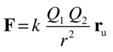
The force law for the electric force between two particles is called Coulomb’s law. It is virtually identical in form with Newton’s law of gravitation, being given by the following, where Q1 and Q2 are the charges on the two particles, r is the distance between them, and k is a constant analogous to G:

Don’t worry about the value of k; we are not going to model real electric charges, but we’ll play around with the force law to see what kind of motion it produces. So we can give k any value we like.
The forces exerted on each particle by the other have the same magnitude but opposite direction, in accordance with Newton’s third law. Like gravity, the force is directed along the line joining the two particles, so Coulomb’s law can be written in vector form in the following two ways, where ru is a unit vector in the direction of r:
or
Here r is the position vector of the object experiencing the force relative to the object that is exerting the force, just like gravity (refer to Chapter 6).
Note the absence of a negative sign in the preceding formula (recall that the equivalent vector formula for gravity had a negative sign). That’s because like charges repel, whereas masses always attract. So if Q1 and Q2 are both positive or both negative, their product is positive, and the force F is a positive number times r. F then is oriented in the direction of r (it is repulsive). But if one of the charges is positive and the other is negative, F is a negative number times r and directed opposite to r (it is attractive).
Let’s create an electric force function similar to the gravity function in the Forces object:
Forces.electric = function(k,q1,q2,r){
     return r.multiply(k*q1*q2/(r.lengthSquared()*r.length()));
}
This is similar in form to the gravity force function, but without the minus sign. As explained previously, the sign of the product q1*q2 determines whether we get an attractive or repulsive force. Just by allowing two different signs for charges, we get a “richer” force than gravity, although the formula is nearly identical in form.
Charged particle attraction and repulsion
To see the electric force in action, let’s build a simulation similar to gravity-field.js, but with electrically charged particles instead of black holes. The new file is electric-field.js. The essential differences are as highlighted below in the init() and calcForce() methods:
function init() {
     // create attractors
     attractors = new Array();
     for (var i=0; i<numAttractors; i++){
          var r = 20*(Math.random()+0.5);
          var charge = (Math.random()-0.5)*1000000;
          if (charge<0){
               color = '#ff0000';
          }else if(charge>0){
               color = '#0000ff';
          }else{
               color = '#000000';
          }
          var attractor = new Ball(r,color,1,charge,true);
          attractor.pos2D = new Vector2D(Math.random()*canvas.width,Math.random()*canvas.height);
          attractor.draw(context_bg);
          attractors.push(attractor);
     }
     // create orbiters
     orbiters = new Array();     for (var i=0; i<numOrbiters; i++){
          var orbiter = new Ball(5, ’#0000ff’,1,1,true);
          orbiter.pos2D = new Vector2D(Math.random()*canvas.width,Math.random()*canvas.height);
          orbiter.velo2D = new Vector2D((Math.random()-0.5)*100,(Math.random()-0.5)*100);
          orbiter.draw(context);
          orbiters.push(orbiter);
     }
     setupGraph();
     t0 = new Date().getTime();
     t = 0;
     animFrame();
}
The main difference is that we are giving the attractors random positive and negative charges, and coloring them blue if their charge is positive and red if their charge is negative (and black if they turn out to have zero charge, which would be a rare occurrence because Math.random() would have to return exactly 0.5 for that to be true). Each moving particle, still called orbiter, is given a positive charge of 1 and is colored blue. So it will be attracted by the red centers and repelled by the blue ones.
In calcForce(), we replace Forces.gravity() by Forces.electric(), and masses by charges:
function calcForce(obj){
     var electric;
     force = Forces.zeroForce();
     for (var i=0; i<numAttractors; i++){
          var attractor = attractors[i];
          var dist = obj.pos2D.subtract(attractor.pos2D);
          if (dist.length() > attractor.radius+obj.radius){
               electric = Forces.electric(k,attractor.charge,obj.charge,dist);
               force = Forces.add([force, electric]);
          }else{
               recycleOrbiter(obj);
          }
     }
}
Figure 10-5 shows an example of what you should see when you run the code.

Figure 10-5. Trajectories in the electric field of multiple charged particles
Electric fields
As with gravity, we can invoke the concept of a force field in electrostatics. Recall that the gravitational field strengthg was defined as the force exerted per unit mass, g = F/m. Similarly, electric field strength E is defined as the force exerted per unit charge:
![]()
Therefore, if we know the electric field strength, we can easily calculate the electric force the field exerts on a particle by multiplying by its charge:
![]()
Compare this with the equivalent formula for gravity:
![]()
Because we want to use the formula F = qE, why not create a force function for it? Let’s call it Forces.forceField:
Forces.forceField = function(q,E) {
     return E.multiply(q);
}
Note that nothing stops us from using the same function to calculate F = mg, too, if we use m for the parameter q and g for E.
Electric field due to a charged particle
As an example, using Coulomb’s law, we can calculate the electric field caused by a charged particle. Let the particle have charge Q. Then the force it exerts on a particle of charge q a distance r away is this:

Therefore, the force per unit charge is this:

In vector form, it can be written as follows:

This is the formula for the electric field produced by a charged particle. But we can also play around with any form for E that we want, without worrying about how it is actually produced. Let’s look at a couple of examples.
The electric field of a stationary charge is constant in time, even though it varies in space, as described in the previous section. This is similar to the gravitational field of a stationary mass. But if a charged particle moves, the electric field it sets up will vary in time. For example, an oscillating charge will produce an oscillating electric field.
A simple example is an electric field that varies in time like a sine or cosine wave. Wave concepts such as frequency and amplitude can then be applied to such a sinusoidally varying field, as discussed in Chapters 3 and 8. Moreover, because an electric field is a vector, its components can vary independently of each other. If all this sounds a bit abstract, that’s because an electric field is an abstract concept! You can’t visualize an oscillating electric field with two or more components as you can visualize an oscillating mass-spring system. Nevertheless, the same math can be applied to both.
Interesting effects can be produced with electric fields that vary in time. In the file electric-field-examples.js, we take a look at the types of motion that different electric fields produce:
var canvas = document.getElementById('canvas'),
var context = canvas.getContext('2d'),
var canvas_bg = document.getElementById('canvas_bg'),
var context_bg = canvas_bg.getContext('2d'),

var particle;
var mass = 1;
var charge = 1;
var E;
var t0, t, dt;
var acc, force;
var graph;
var animId;
var animTime = 25;

window.onload = init;

function init() {
     particle = new Ball(5,'#ff0000',mass,charge,true);
     particle.pos2D = new Vector2D(100,300);
     particle.draw(context);
     setupGraph();
     t0 = new Date().getTime();
     t = 0;
     animFrame();
}
function animFrame(){
     animId = requestAnimationFrame(animFrame,canvas);
     onTimer();
}
function onTimer(){
     dt = 0.001*(new Date().getTime() - t0);
     t0 = new Date().getTime();
     t += dt;
     if (t < animTime){
          move();
     }else{
          stop();
     }
}
function move(){
     moveObject(particle);
     calcForce();
     updateAccel();
     updateVelo(particle);
     plotGraph();
}
function moveObject(obj){
     obj.pos2D = obj.pos2D.addScaled(obj.velo2D,dt);
     context.clearRect(0, 0, canvas.width, canvas.height);
     obj.draw(context);
}
function calcForce(){
     E = new Vector2D(20*Math.sin(1*t),20*Math.cos(1*t));
     force = Forces.forceField(charge,E);
}
function updateAccel(){
     acc = force.multiply(1/mass);
}
function updateVelo(obj){
     obj.velo2D = obj.velo2D.addScaled(acc,dt);
}
function stop(){
     cancelAnimationFrame(animId);
}
function setupGraph(){
     graph = new Graph(context_bg,0,canvas.width,0,canvas.height,0,0,canvas.width,canvas.height); }
function plotGraph(){
     graph.plot([particle.x], [-particle.y], '#666666', false, true);
}
As the preceding code shows, we are moving a charged ball instance under the influence of an electric force specified in calcForce() and plotting its trajectory using the plotGraph() method to draw on a Graph instance previously set up in setupGraph().
Now it’s play time! In the source file we included a number of different sinusoidally varying functions (as commented-out code) for E in calcForce() that you can try. Try the following function to start with:
E = new Vector2D(0, 50*Math.cos(1*t));
What we’re doing is to apply an electric field with a vertical component that varies sinusoidally in time with an amplitude (maximum magnitude) of 50 and a frequency of 1 cycle per second. When you run the code, you’ll see that the particle oscillates up and down in response to the applied electric field.
What happens if we change the amplitude or frequency of the oscillation? If we increase the amplitude, we’ll be applying a larger force, so it’s no surprise that the particle will oscillate with larger amplitude. But the effect of increasing the frequency of the applied electric field might not be so obvious. Try changing the frequency to 3, so that E becomes this:
E = new Vector2D(0, 50*Math.cos(3*t));
If you now run the code, you’ll find that the particle oscillates with a much smaller amplitude. What’s happening here is that the particle, because it has inertia (mass), cannot keep up with the speed of variation of the electric field.
The following function gives a more interesting pattern, by applying an electric field with a constant component of magnitude 1 in the horizontal and a sinusoidally varying vertical component with an amplitude given by 2*t:
E = new Vector2D(1, 2*t*Math.cos(1*t));
This makes the particle accelerate in the horizontal and oscillate with an increasing amplitude in the vertical (see Figure 10-6).

Figure 10-6. Example of the effect of a time-varying electric field on a charged particle
We’ll let you play with the other example functions given in the file, as well as try your own. Of course, there is no reason to restrict yourself to sinusoidally varying functions: feel free to experiment with any function you like.
The electric (electrostatic) force is but one aspect of charged particles. Moving charged particles experience and exert another force—a magnetic force—in addition to the electric force. Therefore, accounting for the magnetic force will change the way that charged particles move. In this section, you’ll see how to compute the magnetic force and how combining it with the electric force affects the motion of charged particles.
We’ve all experienced the fascination of magnets as kids. Part of their appeal is that you can actually feel the force acting between two magnets without them actually touching. Because of this action-at-a-distance characteristic, magnetism fits neatly into the force field concept: a magnet generates a magnetic field around it, which then exerts a force on other magnets and magnetic materials.
What is not obvious at all is that the magnetic field actually has a close connection with the electric field. Magnetic fields are generated by moving charges or by electric fields that vary in time. So, an electric current in a wire will create a magnetic field. A sinusoidally varying electric field will produce a sinusoidally varying magnetic field. The relationship between electric and magnetic fields and the precise way in which they are generated are complex; they are described mathematically by a set of vector differential equations called Maxwell’s equations. To keep things simple, we’ll simply assume given electric and magnetic fields without worrying about how they are produced or how they interact with each other, and focus on how they affect the motion of charged particles.
We already know that the force due to an electric field of strength E on a particle of charge q is given by F = qE. What is the equivalent force law for a magnetic field?
First we need to introduce a magnetic field strength analogous to the electric field strength. There is no need to go into the actual definition; suffice it to say that it exists and is given the symbol B, and that it is a vector like the electric field strength E.
The force on a charge q due to a magnetic field B is then given by the following, where v is the velocity vector of the charged particle and × denotes the cross (vector) product (refer to Chapter 3):
![]()
As explained in Chapter 3, the cross product v × B gives a vector that is perpendicular to both v and B (it points in a direction perpendicular to the plane containing the vectors v and B). Multiplying this by q gives a vector in the same direction but with q times its magnitude. From Chapter 3, the magnetic force can also be written thus, where θ is the angle between the v and B vectors and n is the unit vector perpendicular to v and B vectors and oriented according to the right-hand rule (refer to Chapter 3):
![]()
Note that because the magnetic force is always perpendicular to the particle velocity, it therefore acts as a centripetal force, causing rotation (refer to Chapter 9). Therefore, we can equate the magnetic force law with the centripetal force formula:
Rearranging this equation gives this:

This gives the radius of the trajectory that the charged particle follows. The formula tells us that the radius of the circle increases if the mass or velocity increases, and it decreases if either the charge q or the magnetic field magnitude B increases.
You can combine the electric and magnetic forces on a charged particle to give a single formula for the electromagnetic force on the particle:
![]()
This is called the Lorentz force equation.
We’ll now create a static force function called lorentz() in the Forces object to implement this force law. The only problem is that the vector product is only defined in 3D, whereas our forces are currently only in 2D. But we can implement the magnetic force qv × B in a restricted way if we assume that the magnetic field B is always pointing either into or out of the screen. The magnetic force is given by qv × B = qvB sin (θ) n (refer to the previous section), where θ is the angle between v and B, and in 2D v is always perpendicular to B if the latter is pointing into or out of the screen. Because sin (90°) = 1, this gives, in that special case, the following, where n is perpendicular to v:
![]()
This means that in JavaScript the magnetic force is given by the following, where vel is the velocity vector v and B is the magnitude of the magnetic field:
vel.perp(q*B*vel.length())
The complete Lorentz force function is then as follows:
Forces.lorentz = function(q,E,B,vel) {
     return E.multiply(q).add(vel.perp(q*B*vel.length()));
}
Let’s now play with the Lorentz force function. The file lorentz-force.js sets up a particle and makes it move under the Lorentz force. It is very similar to the previous code in electric-field-examples.js, with the significant differences being in the calcForce() method:
function calcForce(){
     E = new Vector2D(0,0);
     B = 0.2;
     force = Forces.lorentz(charge,E,B,particle.velo2D);
}
We initialized the velocity of the particle to be 40 px/s in the x direction in init(); different results will be obtained for different choices of initial velocity.
Let’s try using different values and math functions for E and B to see what we get. To begin with, let E be a zero vector and let B = 0.2 as in the previous code snippet—in other words, we have a constant magnetic field. Run the code and you’ll see that the particle traces out a circular path, as discussed in the previous section. You can verify what we said at the end of the previous section by increasing the value of B to 0.5 and noting that the radius of the circular path decreases.
You can reduce the velocity of the particle on each timestep by adding the following line in calcForce() or updateVelo():
particle.velo2D = particle.velo2D.multiply(0.999);
This will give you the spiral pattern shown in Figure 10-7.
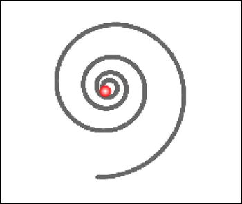
Figure 10-7. A spiral traced by a particle with decreasing velocity in a constant magnetic field
Now add in a non-zero electric field; for example:
E = new Vector2D(1,0);
B = 0.5;
This will produce a helical trajectory. You can also make the electric field and/or the magnetic field time-varying functions; for example:
E = new Vector2D(0,50*Math.cos(1*time));
B = 0.5;
This will produce trajectories that are not always what you might expect. Have fun experimenting!
Other force laws
So far in this chapter, we have discussed physical forces that actually exist in nature. But there is no reason why we cannot invent our own. Because our main purpose is to play around with forces and their effects, we don’t have to be limited by reality. In the next few sections, we’ll introduce different force laws and see what they can do. Feel free to create your own!
Central forces
A central force is one that satisfies the following two conditions:
- The magnitude of the force depends only on the distance from a given point.
- The direction of the force is always toward that point.
Newtonian gravity, electrostatic forces, and spring forces are all examples of central forces. Mathematically, the above two conditions can be combined to give the force vector at any point P as follows, where ru is a unit vector of the point P from the force center, r is its distance from that center, and f(r) is a function of r:
![]()
As you already know, for gravity and electrostatic forces, f (r) is proportional to 1/r 2:

This is usually referred to as an inverse square law. Ever wondered what things would be like if gravity obeyed a different law—for example, an inverse 1/r or an inverse cube 1/r 3 law? Well we can easily find out by creating a modified force function for gravity. But rather than creating special functions for these different cases, let’s create a general central force function that varies according to the following, where both k and n can be positive or negative:
![]()
This gives the following vector form:
![]()
Or equivalently:
![]()
If k is positive, the force is repulsive (because it is in the direction of r); if k is negative, the force is attractive (because it is in the opposite direction from r). If n is positive, the force increases with distance; if n is negative, the force decreases with distance.
Examples include the spring force law, for which k is negative and n is 1; and gravity, for which k is negative and n is –2. The constant k is usually related to some property of the particle (for example, mass or charge).
Let’s add a central force function to the Forces object:
Forces.central = function(k,n,r) {
     return r.multiply(k*Math.pow(r.length(),n-1));
}
The following code snippets from the file central-forces.js set up a particle that is subjected to a central force toward a fixed center:
function init() {
     center = new Ball(2,'#000000'),
     center.pos2D = new Vector2D(350,250);
     center.draw(context_bg);
     particle = new Ball(5,'#ff0000',mass,0,true);
     particle.pos2D = new Vector2D(150,250);
     particle.velo2D = new Vector2D(0,-20);
     particle.draw(context);
     setupGraph();
     t0 = new Date().getTime();
     t = 0;
     animFrame();
}
function calcForce(){
     var r = particle.pos2D.subtract(center.pos2D);
     force = Forces.central(k,n,r);
}
The rest of the code is similar to the previous examples, and include plotting the resulting trajectory of the particle as before. You can experiment with different values for k and n, as well as different initial positions and velocities for the particle.
Can you always make a particle follow a closed orbit with an attractive central force (negative k)? We already know this is possible for an f (r) = k/r 2 law (for example, gravity) and an f (r) = kr law (springs). But what about other force laws, such as f (r) = k/r or f (r) = r 3 ? Try it out and see for yourself!
As an example, with the following initial conditions, and with (k = –1, n = 1), a spring-like force, you get an elongated closed orbit:
center.pos2D = new Vector2D(350,250);
particle.pos2D = new Vector2D(150,250);
particle.velo2D = new Vector2D(0,-20);
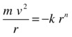
With (k = –100000, n = –2), a gravity-like law, you also get a closed elliptical orbit. But with (k = –1000, n = –1), a 1/r law, you get a flower-like trajectory that does not close on itself (see Figure 10-8); it is a bound orbit, but not a closed one. And with a 1/r3 law you get trajectories that either spiral in or spiral out, but do not close: they are neither closed nor bound. Note that the magnitude of k needs to be adjusted depending on the value of n to produce displacements of the right magnitude to fit on the stage.
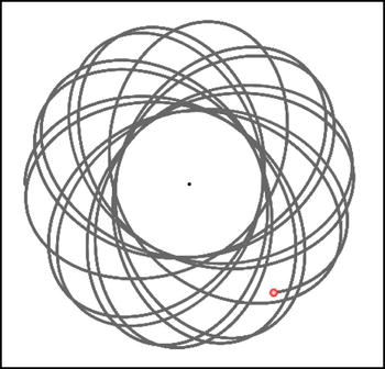
Figure 10-8. Trajectory traced by a particle in a 1/r force field
There is actually a mathematical theorem called Bertrand’s theorem that says the only central force laws that give closed orbits are f(r) = k/r 2 and f (r) = kr laws. Lucky for Earth (and us!) that gravity is a 1/r2 law!
In spite of the last statement, it turns out that closed circular orbits exist, as a special case, for all attractive central forces if you have just the correct tangential velocity. It’s easy to work out the velocity needed for that; just equate the force law with the formula for centripetal force, where m is the mass of the particle:
Solving for v gives this:

You can test this formula with the simulation. It should work for any value of n, provided that k is negative.
Gravity with a spring force law?
Can you imagine what the universe would be like if gravity obeyed a different force law, for instance a spring force law? Well, let’s find out!
The code is in the file spring-gravity.js, and is again adapted from previous examples in this chapter. So we’ll just list it here with little explanation:
var canvas = document.getElementById('canvas'),
var context = canvas.getContext('2d'),
var canvas_bg = document.getElementById('canvas_bg'),
var context_bg = canvas_bg.getContext('2d'),

var vmax = 100;
var m = 1; // particles' mass
var M = 1; // center's mass
var G = 1;
var k = -G*M*m;
var n = 1;
var center;
var particles;
var t;
var t0;
var dt;
var force;
var acc;
var numParticles = 50;

window.onload = init;

function init() {
     // create a stationary center
     center = new Ball(20,'#ff0000',M,0,true);
     center.pos2D = new Vector2D(400,300);
     center.draw(context_bg);
     // create particles
     particles = new Array();
     for (var i=0; i<numParticles; i++){
          var particle = new Ball(4,'#000000',m,0,false);
          particle.pos2D = new Vector2D(Math.random()*canvas.width,Math.random()*canvas.height);
          particle.velo2D = new Vector2D((Math.random()-0.5)*vmax,(Math.random()-0.5)*vmax);
          particle.draw(context);
          particles.push(particle);
     }
     t0 = new Date().getTime();
     t = 0;
     animFrame();
};

function animFrame(){
     requestAnimationFrame(animFrame,canvas);
     onTimer();
}
function onTimer(){
     dt = 0.001*(new Date().getTime() - t0);
     t0 = new Date().getTime();
     t += dt;
     move();
}
function move(){
     context.clearRect(0, 0, canvas.width, canvas.height);
     for (var i=0; i<numParticles; i++){
          var particle = particles[i];
          moveObject(particle);
          calcForce(particle);
          updateAccel(particle.mass);
          updateVelo(particle);
     }
}
function moveObject(obj){
     obj.pos2D = obj.pos2D.addScaled(obj.velo2D,dt);
     obj.draw(context);
}
function updateAccel(mass){
     acc = force.multiply(1/mass);
}
function updateVelo(obj){
     obj.velo2D = obj.velo2D.addScaled(acc,dt);
}
function calcForce(particle){
     var r = particle.pos2D.subtract(center.pos2D);
     force = Forces.central(k,n,r);
}
The main idea here is that we create 50 particles, give them random positions and velocities, and subject them to a central force toward a fixed center. The calcForce() method basically computes a central force, using k = –GMm, where the gravitational constant G = 1, M is the mass of the center; and m is the mass of the relevant particle (all 1 here). Now because k is negative and n = 1, we have a spring force. We’ve created spring-force gravity!
Run the code to get an interesting insight into what life might be like with gravity obeying the spring force law. You’ll see that all the particles are pulled toward the center undergoing some kind of oscillation (see Figure 10-9). If you follow any individual particle you will find that it describes a closed orbit (generally elongated) around the center. If you increase the value of the velocity coefficient vmax, say to 1000, the particles will move about more, but will still be pulled into this oscillatory motion. There is just no way to escape from spring gravity!
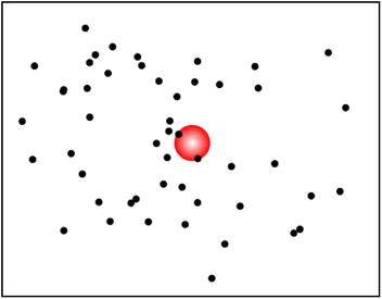
Figure 10-9. Modeling gravity with a spring force
Multiple attractors with different laws of gravity
In our final example, force-fields.js, we’ll combine central forces with different values of k and n to produce a complex force field. This is a universe in which different attractors exert gravity according to different force laws.
Let us first take a look at the init() method:
function init() {
     centers = new Array();
     // k/r force
     var center1 = new Ball(20,'#ff0000',1000,-1,true);
     center1.pos2D = new Vector2D(200,500);
     center1.velo2D = new Vector2D(10,-10);
     center1.draw(context);
     centers.push(center1);
     // k/r2 force
     var center2 = new Ball(20,'#00ff00',100000,-2,true);
     center2.pos2D = new Vector2D(500,100);
     center2.draw(context_bg);
     centers.push(center2);
     // k/r3 force
     var center3 = new Ball(20,'#0000ff',10000000,-3,true);
     center3.pos2D = new Vector2D(600,300);
     center3.draw(context_bg);
     centers.push(center3);
     // create particles
     particles = new Array();
     for (var i=0; i<numParticles; i++){
          var particle = new Ball(4,'#000000',1,0,false);
          particle.pos2D = new Vector2D(Math.random()*canvas.width,Math.random()*canvas.height);
          particle.velo2D = new Vector2D((Math.random()-0.5)*vmax,(Math.random()-0.5)*vmax);
          particle.draw(context);
          particles.push(particle);
     }
     t0 = new Date().getTime();
     t = 0;
     animFrame();
}
As in spring-gravity.js, we set up a bunch of particles (50 in fact) and give them random positions and velocities, with the maximum velocity magnitude vmax set at 20. Then we set up three attractors, called center1, center2, and center3, put references to them in an array called centers, and give them masses of 1000, 100000, and 10000000; and charges of –1, –2, and –3, respectively. The values of the charges are used to store the values of n, the central force law index. There is no reason why we can’t do that because we won’t be using charge here. This means that the attractors will exert 1/r, 1/r 2, and 1/r 3 force laws, respectively.
We give center1 a non-zero velocity and make it move by including the following bolded line of code in the move() method:
function move(){
     context.clearRect(0, 0, canvas.width, canvas.height);
     moveObject(centers[0]);
     for (var i=0; i<numParticles; i++){
          var particle = particles[i];
          moveObject(particle);
          calcForce(particle);
          updateAccel(particle.mass);
          updateVelo(particle);
     }
}
The calcForce() method looks like this:
function calcForce(particle){
     var central;
     force = Forces.zeroForce();
     for (var i=0; i<centers.length; i++){
          var center = centers[i];
          var k = -G*center.mass*particle.mass;
          var n = center.charge;
          var r = particle.pos2D.subtract(center.pos2D);
          if (r.length() > center.radius){
               central = Forces.central(k,n,r);
          }else{
               central = Forces.zeroForce();
          }
          force = Forces.add([force, central]);
     }
}
This is similar to the previous example, except that we now have an array of attracting centers (see Figure 10-10), so we sum the central force that each exerts in a for loop in calcForce(). Note that we are setting the force to be zero if a particle happens to be within a center. This is to improve the visual effect. After all, it’s a universe of our own creation, so we can do whatever we want, can’t we?
Figure 10-10. Particles moving in a field composed of different central forces
If you run the code, you’ll see that most of the particles gravitate around the center that exerts the 1/r force. As it moves along, it captures more particles. The gravity of this attractor dominates because a 1/r force is a longer-range force than a 1/r 2 or a 1/r 3 force: it decays less rapidly with distance. The attractor that exerts the 1/r3 force holds onto very few particles: its influence decays very rapidly with distance.
There are tons of other things you could try; for example, make the attractors move in more complicated ways (for example, orbit a center or move around and bounce). You could add more attractors or include antigravity. You are limited only by your imagination.
Summary
You now have plenty of tools with a whole lot of forces for creating interesting types of motion. This concludes Part II of the book. In Part III, you will apply what you have learned in Part II to build more complex systems consisting of interacting particles or extended objects.