![]()
Restoring Forces: Springs and Oscillations
Springs are among the most useful tools you’ll come across, especially for creating interesting physics effects. A great many systems can be modeled using springs and spring-like motion. Therefore, learning the basics of spring motion is time well spent. But beware: springs are strangely addictive!
Topics covered in this chapter include the following:
- Free oscillations: An object will oscillate under the action of a spring force, also known as a restoring force.
- Damped oscillations: Damping dissipates the energy of oscillations so that they die out with time.
- Forced oscillations: Oscillations can be driven by external forces that sustain them against damping forces.
- Coupled oscillators: Interesting effects can be produced by using multiple springs and objects coupled together.
Springs and oscillations: Basic concepts
We introduced oscillations back in Chapter 3, while discussing sinusoidal waves and their combinations (refer to the section “Using trig functions for animation”). An oscillation is a repeating motion around some central position. Simple examples of oscillating systems include a pendulum and a swing.
Oscillations abound in natural systems, too: trees oscillate under a blowing wind, and floating objects oscillate on the water surface because of passing waves. Man-made mechanisms that include springs involve oscillations. Hence, there is an intuitive association between oscillations and springs; in fact, we will use the terms oscillations and spring-like motion interchangeably. This association is more than verbal: oscillating systems can usually be modeled using virtual “springs.”
You’ve already met spring-like motion in this book, probably without realizing it. The floating ball simulation in the preceding chapter provided an example in which the ball oscillated on the water surface in a spring-like fashion. Many other things undergo spring-like motion: the suspension mechanism of a car; and the swaying of a tree, its branches, and their leaves in the wind. Other things, although they don’t necessarily appear to be spring-like, can nevertheless be modeled using springs: deformable bodies such as ropes, clothes, and hair. Surely then, there must be common characteristics that these systems exhibit that make them amenable to modeling using springs. So, what are the general characteristics of oscillating systems?
Restoring force, damping, and forcing
An oscillating system will usually involve the following ingredients:
- An equilibrium position in which an object would remain if it were not moving.
- A restoring force that pulls the object back toward the equilibrium position if it is displaced.
- A damping force that reduces the oscillations with time.
- A driving force that displaces the object from its equilibrium position.
Of those, the first two are essential to generate oscillations, whereas the last two may or may not be present, depending on the system. Although more complex systems may not appear to show these characteristics, they can be composed of (or be modeled by) component parts that do—for example, a rope can be represented as a chain of springs.
In understanding the roles of the restoring force, damping, and forcing, a relevant concept is that of amplitude. The amplitude of an oscillation is the maximum displacement from the equilibrium position. If you pull a swing away from its equilibrium position and then let go, the initial displacement will be the amplitude of the oscillation.
The restoring force changes the displacement with time, but it does not change the amplitude (maximum displacement). The amplitude depends on the amount of energy in the system. A damping force takes away energy from the system and therefore reduces the amplitude with time. This is what would happen if, after initially displacing it, you left the swing to oscillate on its own. A driving force puts energy into the system and therefore tends to increase the amplitude of the oscillations. With both damping and forcing being present, it is possible for the energy put into the system to compensate exactly for the energy lost by damping. In that case, the amplitude remains constant with time, as if only a restoring force were present. In the swing example, this is achieved by pushing the swing periodically with the right amount of force.
In most oscillating systems, the force law that governs the restoring force is known as Hooke’s law (because a gentleman named Robert Hooke discovered it at some point in history).
Hooke’s law is quite simple. We’ll explain it for springs first because that’s the original form of the law. Take a look at Figure 8-1, which shows a spring of natural length l, fixed at one end, that is then stretched by an amount x, so that its length becomes l + x.
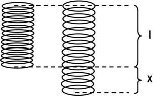
Figure 8-1. A stretched spring experiences a restoring force proportional to the extension x
Hooke’s law says that the spring will be pulled back by a force of magnitude F given by this equation:
![]()
In other words, the restoring force is proportional to the extension x. The constant of proportionality k is known as the spring constant, and it is a measure of the stiffness of the spring. The greater the value of k is, the greater the force will be for a given extension, so that the spring will be pulled back more strongly when stretched.
The minus sign indicates that the force is in the opposite direction to the extension. So if the spring is compressed instead, the force will push back to increase its length.
The vector form of the equation is this, where now r is interpreted as the displacement vector of the free endpoint of the spring:
![]()
For most of what we’ll do in this chapter (and probably for what you’ll want to do, too), we won’t care much about the actual spring. What we’ll be more interested in is the motion of a particle attached to the end of a spring. How would such an object move? As every kid knows, it will oscillate about the equilibrium position.
In fact, we could get rid of the spring altogether and just consider the effect of the restoring force on the particle. This is what we’ll do in many examples. In such a case, the displacement vector r in Hooke’s law is interpreted as the displacement from the equilibrium position about which the particle is oscillating, as shown in Figure 8-2.
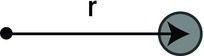
Figure 8-2. A particle oscillating about an equilibrium position
A word of warning before we end this section: it should not be assumed that all oscillations obey Hooke’s law; many don’t. However, a great many types of moving systems follow Hooke’s law, at least approximately. So we’ll stick with Hooke’s law in this chapter.
Let’s start by modeling free oscillations. What that means is that the system oscillates purely under the action of the restoring force, without any other force. Of course, for an object to oscillate, something (an applied force) must have moved it away from its equilibrium position in the first place. But what we are interested in here is what happens after that initial forcing is removed and the oscillating system is left to itself.
To begin with, we need to create a new force function in the Forces object for the restoring force. Let’s call it spring(). It is a very simple function:
Forces.spring = function(k,r){
     return r.multiply(-k);
}
The function spring() takes two arguments, which are the spring constant k and the displacement vector r (this is just the vector r in the previous formulas). It returns the restoring force F = –kr.
Let’s now use that function to create a basic oscillator.
You know what’s coming next, don’t you? Here is some code extracted from the file basic-oscillator.js that creates the object that we want to oscillate as a Ball object called ball (we’re omitting the standard lines on the canvas and context variables). We don’t actually create a spring (in the visual sense) but instead another Ball object that we call attractor, whose position will be the equilibrium position. Both have an initial velocity of zero and are placed some distance apart by giving them different position vectors pos2D:
var ball;
var displ;
var center = new Vector2D(0.5*canvas.width,0.5*canvas.height);
var m = 1;
var kSpring = 1;
var t0, dt;
var acc, force;
var animId;
window.onload = init;

function init() {
     // create a ball
     ball = new Ball(15,'#0000cc',m,0,true);
     ball.pos2D = new Vector2D(100,50);
     ball.draw(context);
     // create an attractor
     var attractor = new Ball(2,'#000000'),
     attractor.pos2D = center;
     attractor.draw(context_bg);
     // make the ball move
     t0 = new Date().getTime();
     animFrame();
}
The animation code is pretty standard; the only novelty is in the calcForce() method:
function calcForce(){
      displ = ball.pos2D.subtract(center);
      force = Forces.spring(kSpring,displ);
}
This code is very simple: it first calculates the displacement vector displ of the object relative to the attractor and then uses it to calculate the spring force that the attractor exerts on the object. The parameter kSpring is the spring constant k.
Run the code and you’ll see the ball oscillate about the attractor, as expected. Now change the spring constant value from 1 to 10. This gives you a stiff spring. If you run the code again, you’ll see the ball oscillate faster. If you want it to oscillate at a different amplitude, just change the initial position in basic-oscillations.js.
Next change the value of k back to 1, then change the initial velocity of the ball to (200,0):
ball.velo2D = new Vector2D(200,0);
When you run the code, you should now see the ball “orbit” the attractor in some sort of oval trajectory. It’s a bit like what you saw with gravity in Chapter 6. Both gravity and the spring force are attractive forces that always act toward a point. But gravity decreases with distance, whereas the spring force increases with distance. That’s because gravity is proportional to 1/r2, whereas the spring force is proportional to r, where r is the distance from the center of attraction.
Simple harmonic motion
The type of oscillatory motion you’ve just seen is technically called simple harmonic motion (SHM). An object undergoes SHM if the only force acting on it is the spring force, as was the case in the previous example.
Because the only force in SHM is the restoring forceF = –kr, and Newton’s second law says that F = ma, these two equations together tell us that for SHM the following is true:
![]()
Dividing both sides of this equation by m gives this:

Here m is the mass of the oscillating particle, and k is the spring constant, so the ratio k/m is a constant. This equation therefore tells us that the acceleration of the oscillating particle is proportional to its displacement vector from the center. The constant of proportionality is negative, meaning that the acceleration is always opposite to the displacement vector (it always points toward the center because the displacement vector always points away from the center by definition). See Figure 8-3.
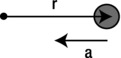
Figure 8-3. The acceleration in SHM always points toward the center, opposite to displacement
Remember back in Chapter 3 where we talked about derivatives and said that acceleration is the second derivative of displacement? This means the following is true:

Therefore we can write the SHM equation a = –(k/m)r in the equivalent form:
Stating it this way makes it clear that the equation that governs SHM is a second-order differential equation, as described in Chapter 5. What the animation code in basic-oscillator.js has been doing is to solve this second-order differential equation numerically using the Euler scheme (again as described in Chapter 5).
In fact the preceding differential equation can also be solved analytically to give a formula for the displacement as a function of time. This is an exercise in college-level calculus, and here is the solution, where A and B are constant vectors that depend on the initial conditions, and ω is the angular velocity of the oscillation (see Chapter 3):
![]()
Hence, SHM consists of the sum of a sine and a cosine function. This is not surprising because SHM is basically an oscillatory motion and, as you know from Chapter 3, sin and cos are oscillatory functions. The value of ω sets the frequency and therefore the period of oscillation, whereas the values of A and B set the amplitude of the oscillations (the maximum displacement of the object from its equilibrium position).
Anyone with a little knowledge of calculus can immediately write down the velocity vector v by differentiating the preceding expression for r because v = dr/dt. The result is this:
![]()
What are the values of A, B, and ω? A and B are set by the initial conditions that you specify for the displacement and velocity of the object at the start (the values of r and v at time t = 0). Let’s call the initial displacement vector r0 and the initial velocity vector v0. If we now put t = 0 into the preceding equations for r and v because cos(0) = 1 and sin(0) = 0, we get this:
![]()
We also get the following:
![]()
This tells us right away that A = r0 and B = v0/ω.
If you were to solve that differential equation, you would also find that the angular velocity ω is actually given by this formula:

This is called the natural frequency of the system. If the oscillating system is given an initial perturbation (to move the object away from its equilibrium position), but is thereafter left on its own, it will oscillate at that frequency and only at that frequency in the absence of other influences such as damping.
Now, if you remember (again from Chapter 3) that ω = 2πf and f = 1/T, where f is the frequency (the number of oscillations per second) and T is the period of oscillation (the time to complete one oscillation), you can use the preceding formula to obtain both the frequency and period of the oscillation in terms of the parameters k and m:


These formulas tell you that if you increase the spring stiffnessk, the frequency of the oscillations will increase and its period will decrease (it will oscillate faster). If you increase the mass of the oscillating particle instead, the reverse will happen, and it will oscillate more slowly. Go ahead and try it!
These are the only two parameters that affect the frequency and period; the initial position and velocity of the object do not. You might think that if the object is initially farther away from the center it will take longer to complete one oscillation. But not with SHM. What happens is that if the object is farther away, it experiences a greater acceleration at the start so that on average it acquires a greater velocity, which compensates for the longer distance it has to travel to complete one oscillation. Skeptical? Try it by timing the oscillations with a stopwatch or outputting the time.
In fact, we can do better than that. Let’s plot a graph.
Oscillations and numerical accuracy
To plot a graph, we modify basic-oscillations.js by changing the initial position of the oscillating object as follows:
object.pos2D = new Vector2D(100,50);
We also alter the position of the attractor:
var center = new Vector2D(0.5*canvas.width,50);
After adding some extra bits of code to plot a graph showing the displacement of the object against time, and to run the simulation for a fixed duration (20 s), we then save the file as free-oscillations.js.
Here is the code that sets up and plots the graph:
function setupGraph(){
     //graph= new Graph(context,xmin,xmax,ymin,ymax,xorig,yorig,xwidth,ywidth);
     graph = new Graph(context_bg,0,20,-250,250,50,300,600,300);
     graph.drawgrid(5,1,50,50);
     graph.drawaxes('t (s)','displacement (px)'),
}
function plotGraph(){
     graph.plot([t], [displ.x], '#ff0000', false, true);
     graph.plot([t], [displ.y], '#0000ff', false, true);
}
The plotGraph() method, which is called at each timestep, invokes the plot() method of Graph to plot the x and y coordinates of the displacement of the ball relative to the attractor.
If you now run the code, you’ll see something like Figure 8-4. Sure enough, the horizontal displacement (x) of the object with time is a sinusoidal wave, as we said in the previous section. The vertical displacement is always zero because of the initial condition we chose. But it’s easy to change it by giving the object an initial vertical component of velocity or a different initial vertical position. Then the y displacement would also vary sinusoidally. You can also change the values of k, m, and the initial position of the object to verify the statements we made at the end of the previous section about how the frequency and period of oscillations vary (or not) with these parameters.
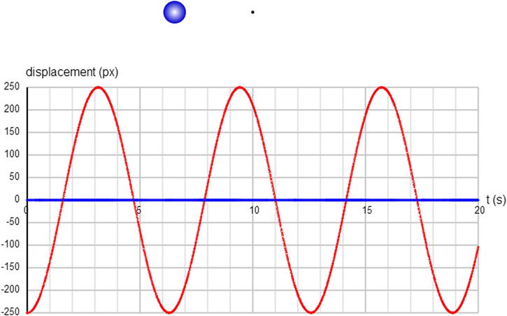
Figure 8-4. Plotting the displacement of an oscillating object as a function of time
Let’s now see how accurate our simulation is by comparing the trajectory of the oscillating object with what the analytical solution given in the previous section predicts.
To do this, we first modify free-oscillations.js to free-oscillations2.js by changing the initial velocity of the oscillating object as follows:
object.velo2D=new Vector2D(0,50);
Then we add code that calculates the values of A, B, and ω (defined as variables A, B and omega in the code) using the previously given equations ![]() , A = r0 , and B = v0/ω. This is done in the init() method, which therefore contains these additional lines:
, A = r0 , and B = v0/ω. This is done in the init() method, which therefore contains these additional lines:
omega = Math.sqrt(kSpring/m);
A = ball.pos2D.subtract(center);
B = ball.velo2D.multiply(1/omega);
We then modify the code to create two Graph objects graphX and graphY (set up in a suitably modified setupGraph() method), on which we plot the x and y displacements, respectively, in plotGraph(). In the plotGraph() method, we then insert the following additional lines to plot the x and y components of the analytical solution r = A cos (ωt) + B sin (ωt):
var r = A.multiply(Math.cos(omega*t)).add(B.multiply(Math.sin(omega*t)));
graphX.plot([t], [r.x], '#00ff00', false, true);
graphY.plot([t], [r.y], '#ff00ff', false, true);
If you now run the code, you’ll see the object orbiting the attractor in an elongated orbit, and you’ll see a pair of graphs for each of the horizontal and vertical displacements of the object. In each pair of graphs, one corresponds to the analytical solution computed by the specified formulas, whereas the other corresponds to the numerical solution as computed by the simulation. You can see that they are quite close to each other, practically overlapping (see Figure 8-5). Euler integration is not doing such a bad job in this case.

Figure 8-5. Comparing the numerical and analytical solutions for the oscillator
However, if you now change the value of kSpring to 20, for example, so that the “spring” is stiffer and the object moves faster, you’ll see that the difference between the two is more significant, signaling that Euler is losing accuracy. If you try a value for kSpring greater than about 100, then you may find that Euler gives you complete rubbish, and the object ends up in the wrong place at the wrong time. So here you begin to see that you can get the wrong physics if you are not careful with your integrator, especially in the case of springs. You’ll see how to overcome this problem in Chapter 14. Meanwhile, for the rest of this chapter we’ll avoid very high values of the spring constant.
In the previous examples, the oscillations just go on forever. In practice, this rarely happens. Oscillating systems are usually damped. That means the oscillations are reduced and die out in time as energy is removed from the system. This is similar to the drag force, which dissipates the kinetic energy of a moving object and makes it slow down. To implement damping in our springs, we need a damping force.
The damping force is usually modeled as being proportional to the velocity of the moving object. This means that, at any instant in time, it is given by the following equation, where c is a constant known as the damping coefficient, and the minus sign indicates that the force is in the opposite direction to the velocity:
![]()
Notice that this is exactly the same form as the force law for linear drag. We could, therefore, use the linearDrag() function to implement damping in spring motion. However, although drag is certainly a form of damping, it is not physically the only form of damping, although the two terms are sometimes used interchangeably. Drag is the resistive force exerted by a fluid on a moving object immersed in it. Spring damping, on the other hand can be caused by external factors such as fluid drag or external friction, or to internal factors such as internal friction, which arise from the molecular material properties of springs. In fact, you could have both internal damping due to spring resistance and drag due to fluid resistance side by side (with different coefficients, of course). For example, a mass suspended on a spring and oscillating in a fluid such as air or water experiences both internal friction and fluid drag. For these reasons, we prefer to create a separate function for damping. The form of this function is identical to that for linearDrag(), as shown in this listing:
Forces.damping = function(c,vel){
     var force;
     var velMag = vel.length();
     if (velMag>0) {
          force = vel.multiply(-c);
     }
     else {
          force = new Vector2D(0,0);
     }
     return force;
}
The effect of damping on oscillations
We’ll now modify free-oscillations.js to handle damping in addition to the spring force. The new file is called damped-oscillations.js, and basically introduces a new force: damping. So one difference from free-oscillator.js is that it declares a damping coefficient cDamping and assigns it a value:
var cDamping = 0.5;
The other difference is that it includes a damping force in calcForce() and adds it to the spring force to work out the resultant force:
function calcForce(){
     displ = ball.pos2D.subtract(center);
     var restoring = Forces.spring(kSpring,displ);
     var damping = Forces.damping(cDamping,ball.velo2D);
     force = Forces.add([restoring, damping]);
}
That’s it. If you run the code with kSpring = 10 and cDamping = 0.5, you’ll see something like what’s shown in Figure 8-6. The oscillations die out in time, and the object eventually settles at the equilibrium position, as you’d expect.

Figure 8-6. Damped oscillations
At this point, you should play with the damping constant cDamping to see what you get. Choose a lower value, and you’ll see the oscillations persist longer, whereas a higher value will kill them off sooner. You might think that the greater the value of c, the quicker the object will stop. In fact, there is a critical value of c for which the oscillations die in the minimum time. At this value, there are no oscillations at all. The object simply moves smoothly to the equilibrium position without oscillating beyond it. This is called critical damping, and an example is shown in Figure 8-7. For kSpring = 10 in our simulation, the critical value of cDamping is about 5.5, and the object reaches its equilibrium position in about 1.5 seconds. If you increase cDamping beyond this critical value, for example to 10 or 20, you’ll see that the object actually takes longer to reach its equilibrium location. This is because the increased damping slows it down so much that, although it does not go beyond the equilibrium position, it takes longer to get there. Critical damping is a very useful phenomenon that’s applied in things like damping mechanisms in doors.
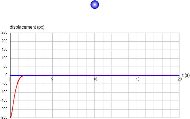
Figure 8-7. Critical damping
Analytical solutions for oscillations with damping
This brief section is for enthusiasts. You may safely skip it if complicated formulas are not your thing. The point of this section is to show you how the analytical solution quoted previously for free oscillations changes in the presence of damping, and how well our simulation does at reproducing it. Thus, it is more educational than practical.
Newton’s second law for oscillations under a spring force F = –kr, together with a damping force F = –cv is the following:
![]()
This can be written in terms of derivatives as (after dividing both sides by m):
The analytical solution of this differential equation is given by the following:
![]()
where the constants γ, ω0, ωd, A and B are given by the following:


![]()
![]()
Comparing this with the previous solution without damping, you’ll notice that there is an additional exponential factor in the expression for r, which is responsible for the decay in the sinusoidal oscillations (see Chapter 3). The new parameter γ is due to the damping. In the absence of damping, c = 0 and so γ = 0; the solution then reduces to that without damping. Note also that the angular frequency of the oscillations is now ωd (because it appears in the sine and cosine), which is less than the natural frequency ω0 in the absence of damping (which was previously denoted by ω).
We coded up these equations in a modified version of free-oscillations.js that we call damped-oscillations2.js. Take a look at the code if you wish. If you run the code, you’ll find that there is again some discrepancy between this analytical solution and the numerical solution computed by the simulation. In fact, sometimes you might find that the oscillating object goes seemingly wild, ending up in places it shouldn’t be. The important take-away message from all this is that Euler integration simply does not cut it when it comes to simulations like this, except for the simplest motions. In Chapter 14, we shall discuss alternative integration schemes that overcome this problem.
In the presence of damping, the oscillations of a system will die out in time. Therefore, a force is needed to sustain oscillations or to initiate them in the first place. That’s called a driving force, or forcing.
Driving forces can be of any form, so let’s denote them simply by f (t). This simply means that the force is a function of time without specifying the form of the force law at all.
For example, we could have a periodic force of the form f = A cos (ωt) + B sin (ωt), where A and B are constant vectors that give the amplitude (maximum magnitude) and direction of the force, and ω is the angular frequency of the forcing. This could, for example, represent an oscillator interacting with and driving another, such as a periodic wind blowing over a suspension bridge and causing it to vibrate.
Let’s start with an example.
Example: A periodic driving force
We’ll start by modifying damped-oscillations2.js. We do not want to plot the analytical solutions here, so we get rid of the relevant lines in plotGraph(), but we’ll keep the three lines that compute gamma, omega0, and omegad in the init() method. These are the variables corresponding to the constants γ, ω0, and ωd. After deleting any unnecessary variable declarations, we rename the file as forced-oscillations.js.
Remember that omega0 (ω0) is the natural angular frequency of the undamped system, and omegad (ωd) is the angular frequency with damping. Let’s begin by adding the following lines to calcForce():
var forcing = new Vector2D(200*Math.cos(2*omegad*t)+200*Math.sin(2*omegad*t),0);
force = Forces.add([restoring, damping, forcing]);
This adds a driving force of the form f = A cos (ωt) + B sin (ωt), with A and B both of magnitude 200 and in the x direction (we need fairly large values to see a noticeable difference of the forcing on the oscillations), and ω = 2 ωd. So we are forcing the system with a driving force that varies sinusoidally with time at an angular frequency that is twice the frequency of the damped system.
Run the code, and you’ll see that the oscillations start to die out as they did before without the forcing. Then, after a while, the object starts to oscillate at around twice the frequency it did before, but with a much smaller amplitude. This carries on indefinitely. So, the effect of the sinusoidal driving force is to eventually make the system oscillate at the driving frequency (albeit at reduced amplitude), rather than the frequency that the system would prefer to oscillate at on its own. You can try this with different forcing frequencies. For example, if you use ωd/2, half the damped system’s frequency, the oscillations will eventually have a frequency of half the initial, unforced frequency. The conclusion is that if you force a system to oscillate at a frequency other than its natural frequency, it will still oscillate but at a reduced amplitude.
Now make the forcing frequency exactly equal to ωd by modifying the forcing vector to this:
var forcing = new Vector2D(200*Math.cos(omegad*t)+200*Math.sin(omegad*t),0);
When you run the code, you’ll now see that the oscillations quickly settle into equilibrium at the original frequency ωd and maintain a large, constant amplitude without decaying. The system is now “happy” because it is forced at exactly the frequency it likes to oscillate. Hence, it settles down quickly and oscillates with a large amplitude. So, although damping reduces the energy of the system, forcing puts energy back into the system and sustains the oscillations.
When the forcing frequency is equal to the natural frequency of the oscillating system, we have what is called resonance. It happens in lots of situations, from pushing a child’s swing to the tuning of radio circuits. Resonance can have bad effects, too, such as unwanted vibrations in bridges due to periodic wind gusts. In fact, resonance due to wind gusts was infamously responsible for the collapse of the Tacoma Narrows Bridge in Washington in 1940.
Example: A random driving force
Next, let’s try a random forcing. This is as easy as replacing one line of code. Let’s try this first:
var forcing = new Vector2D(1000*Math.random(),0);
This applies a random force of up to 1,000 units in the positive x direction (to the right). If this were the only force, it would send the object flying off to the right, never to be seen again. But the presence of the restoring force (as its name suggests) pulls the object back toward the attractor. In fact, because the restoring force is proportional to the displacement from the attractor, the farther away the object moves, the stronger it gets pulled back. This creates an interesting effect that you’ll surely want to experiment with. Because we made the force act only to the right, the object will spend most of its time on the right side of the attractor, although it occasionally gets pulled slightly to the left.
To make the oscillations more symmetrical around the attractor, simply change that line of code to this:
var forcing = new Vector2D(1000*(Math.random()-0.5),0);
This produces a random force with an x component between –500 and +500, where the minus sign means that the force is directed to the left instead of to the right. Run the code, and you’ll get a nonperiodic oscillator (the object oscillates without regularity).
Finally, let’s make the object oscillate under a random force in 2D by modifying the same line of code to the following:
var forcing = new Vector2D(1000*(Math.random()-0.5),1000*(Math.random()-0.5));
If you run the code, you’ll see that the system quickly goes into a state where the oscillations in the x and y directions are of comparable magnitude, with the object hovering around the attractor (see Figure 8-8). The object is kicked in different directions at every timestep, but it is also pulled back toward the attractor. It’s not allowed to get away, no matter how large the forcing is, because the farther it goes the more strongly it gets pulled back. That’s an interesting effect. It’s some kind of crazy random orbiting motion. Or maybe even like a bee buzzing around a flower. Play with that one for sure!
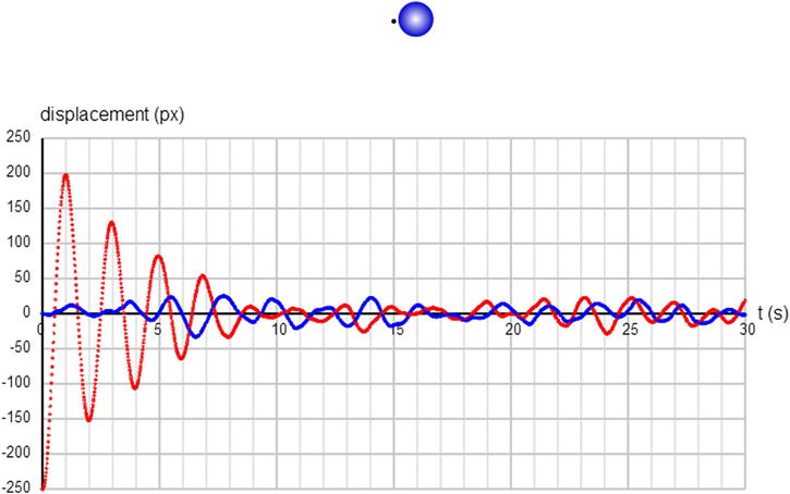
Figure 8-8. Oscillator with random forcing
Gravity as a driving force: bungee jumping
Let’s now move on to something a little different: bungee jumping! Someone jumps off a bridge or similar structure tied to an elastic cord whose other end is tied to a fixed support on the structure. The elastic cord has a natural unstretched length, say cordLength. So if the distance of the jumper from the fixed support is less than cordLength, gravity and drag are the only forces on the jumper. But once that distance exceeds cordLength, the elastic (spring) force will come into effect, and pull the jumper back.
So here gravity is acting as the driving force, so that f(t) = mg, where m is the mass of the jumper. It’s a constant forcing, unlike the types of forcing discussed before. The main damping mechanism is provided by drag through the air, so it can be implemented using the Forces.drag() method. Finally, the spring force is applied only if the jumper’s distance from the fixed support exceeds the natural unstretched length of the cord, cordLength. This distance may be less than cordLength initially (before the jumper jumps off some supporting structure), but also whenever the jumper bounces back high enough.
Because this example is a little different from the last few, we’ll list the full source code and then go through the main points. The file is called simply bungee.js:
var canvas = document.getElementById('canvas'),
var context = canvas.getContext('2d'),

var jumper;
var fixedPoint;
var displ = new Vector2D(0,0);
var center = new Vector2D(0.5*canvas.width,50);
var mass = 90;
var g = 20;
var kDamping = 0.02;
var kSpring = 25;
var cordLength = 100;
var t0, dt;
var acc, force;
var animId;
window.onload = init;

function init() {
     // create a bungee jumper
     jumper = new StickMan();
     jumper.mass = mass;
     jumper.pos2D = center;
     jumper.draw(context);
     // create a fixedPoint
     fixedPoint = new Ball(2,'#000000'),
     fixedPoint.pos2D = center;
     fixedPoint.draw(context);
     // make the ball move
     t0 = new Date().getTime();
     animFrame();
};

function animFrame(){
     animId = requestAnimationFrame(animFrame,canvas);
     onTimer();
}
function onTimer(){
     var t1 = new Date().getTime();
     dt = 0.001*(t1-t0);
     t0 = t1;
     if (dt>0.2) {dt=0;};
     move();
}
function move(){
     context.clearRect(0, 0, canvas.width, canvas.height);
     drawSpring(jumper);
     moveObject(jumper);
     calcForce(jumper);
     updateAccel();
     updateVelo(jumper);
}
function drawSpring(obj){
     fixedPoint.draw(context);
     context.save();
     if (displ.length() > cordLength){
          context.lineStyle = '#999999';
          context.lineWidth = 2;
     }else{
          context.lineStyle = '#cccccc';
          context.lineWidth = 1;
     }
     context.moveTo(center.x,center.y);
     context.lineTo(obj.x,obj.y);
     context.stroke();
     context.restore();
}
function moveObject(obj){
     obj.pos2D = obj.pos2D.addScaled(obj.velo2D,dt);
     obj.draw(context);
}
function calcForce(obj){
     displ = obj.pos2D.subtract(center);
     var gravity = Forces.constantGravity(mass,g);
     var damping = Forces.drag(kDamping,obj.velo2D);
     var extension = displ.subtract(displ.unit().multiply(cordLength));
     var restoring;
     if (displ.length() > cordLength) {
          restoring = Forces.spring(kSpring,extension);
     }else{
          restoring = new Vector2D(0,0);
     }
     force = Forces.add([gravity, damping, restoring]);
}
function updateAccel(){
     acc = force.multiply(1/mass);
}
function updateVelo(obj){
     obj.velo2D = obj.velo2D.addScaled(acc,dt);
}
Notice that we are creating two objects here: a fixed point and a jumper. The jumper is an instance of StickMan, a poor man’s version of a man, which you are welcome to improve upon by editing the file stickman.js.
First, note the large value we used for the spring constant kSpring (25). That’s because we’ve specified the mass of the jumper as 90 in bungee.js, instead of 1 as in all the previous simulations. This mirrors the fact that, if you want to make a big guy oscillate at the end of an elastic cord, the cord had better be pretty stiff!
Looking next at the calcForce() method, we see that we are including gravity, damping, and restoring forces, as discussed previously. The first two are implemented in a straightforward way as usual. There are two differences in how we calculate the restoring force compared with earlier examples. First, the displacement vector that must be used to calculate the restoring force is now the displacement vector of the end point of the elastic cord (the extension), as explained at the beginning of this chapter, not the displacement of the object from the fixed support. Therefore, we first calculate that extension as a vector in the following line:
var extension = displ.subtract(displ.unit().multiply(cordLength));
Note the cunning use of the unit() method, newly added to the Vector2D object, where vec.unit() returns a vector of unit length in the direction of vector vec.
We then supply extension as the second argument in Forces.spring().
The second difference is that the restoring force is nonzero only if the object is farther from the support than the length of the cord. That’s the same as saying that displ.length() > cordLength. This explains the code within the if block:
if (displ.length() > cordLength) {
     restoring = Forces.spring(kSpring,extension);
}else{
     restoring = new Vector2D(0,0);
}
The other new feature is that we’ve included a drawSpring() method, called within the move() method, that draws a line to represent the elastic cord at each timestep. The line is drawn thinner and fainter when the cord is unstretched. As usual, run the code and feel free to play with the parameters. The initial position of the object is the same as that of the fixed support. This makes the object oscillate in a vertical straight line (it makes the oscillations 1D). To make it 2D, simply change the initial x-coordinate of the object in bungee.js; for example:
object.pos2D = new Vector2D(300,50);
A screenshot of the demo is shown in Figure 8-9.
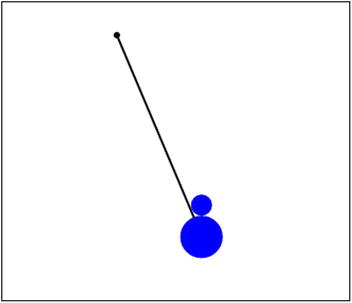
Figure 8-9. A bungee jump simulation
Example: Driving force by user interaction
User interaction can also be viewed as some kind of forcing. In the following example, we will build a simulation in which the user can click and drag the object and release it in any location. This will disturb the system, setting it to oscillate.
It is fairly straightforward to modify the bungee simulation to do what we want here. We’ll call the new file dragging-oscillations.js. Among other modifications, we change the mass of the object to 1 and add code to enable dragging. Take a look at the file if you want to see how this is done—the details are not particularly interesting for our present purposes. The main point here is that the code changes enable you, the user, to exert a driving force whenever you feel like by dragging and releasing the object. Hence, the forcing is not specified by a mathematical function but is a product of random human interaction.
The essential physics does not change, however, as reflected in the calcForce() method:
function calcForce(obj){
     displ = obj.pos2D.subtract(center);
     var gravity = Forces.constantGravity(mass,g);
     var damping = Forces.drag(kDamping,obj.velo2D);
     var extension = displ.subtract(displ.unit().multiply(springLength));
     var restoring = Forces.spring(kSpring,extension);
     force = Forces.add([gravity, damping, restoring]);
}
In calcForce(), we include gravity as before, while damping is included using the Forces.damping() function. We then calculate the extension of the spring and feed it into the restoring force as before. However, because this is a spring that can also be compressed and is not an elastic cord, we apply the restoring force even if the extension is negative, so we have deleted the if statement we had in the previous bungee example.
Run the code and you’ll see the object fall down under gravity and be pulled back again by the spring, oscillating with reducing amplitude due to the damping. If you drag the object and release it, it oscillates again thanks to the forcing.
Coupled oscillators: Multiple springs and objects
In all the examples so far, we’ve considered only a single object and spring system. Effects get even more interesting when you couple more than one object and spring system together. In fact, you can create extended systems based on objects with masses connected by springs. In the next subsection, you’ll see an example of what can be done. Then we’ll look at more complicated examples in Chapter 13 when we model deformable bodies.
Example: A chain of objects connected by springs
What you’ll create is shown in Figure 8-10: a number of balls connected by springs, with the first ball connected to a support. The support will then be moved around, causing the chain of suspended balls to move around, too.
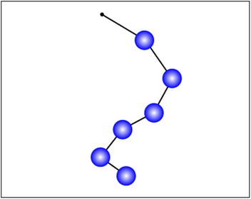
Figure 8-10. A chain of objects held together by springs
The forces that will be modeled include gravity, damping, and restoring force. The springs will have a natural length, as in the last couple of examples. Each ball will therefore experience gravity, damping, a restoring force due to a spring above, and another restoring force due to a spring below (except for the last ball). The springs themselves will be assumed to be massless.
The code is in a file called coupled-oscillations.js. We first list the variable declarations and init() function:
var canvas = document.getElementById('canvas'),
var context = canvas.getContext('2d'),

var balls;
var support;
var center = new Vector2D(0.5*canvas.width,50);
var g = 20;
var kDamping = 0.5;
var kSpring = 10;
var springLength = 50;
var numBalls = 6;
var t0, t, dt;
var acc, force;
var animId;

window.onload = init;

function init() {
     // create a support
     support = new Ball(2,'#000000'),
     support.pos2D = center;
     support.draw(context);
     // create a bunch of balls
     balls = new Array();
     for (var i=0; i<numBalls; i++){
          var ball = new Ball(15,'#0000ff',1,0,true);
          ball.pos2D = new Vector2D(0.5*canvas.width,100+60*i);
          ball.pos2D = new Vector2D(0.5*canvas.width+60*i,100+60*i);
          ball.draw(context);
          balls.push(ball);
     }
     // make the balls move
     t0 = new Date().getTime();
     t = 0;
     animFrame();
}
As in the previous two examples, we first create a Ball object to act as a support. Then we create a whole bunch of Ball objects and put them in an array called balls.
We’ve made a few structural changes to the animation part of the code, which we also reproduce here in full for ease of reference:
function animFrame(){
     animId = requestAnimationFrame(animFrame,canvas);
     onTimer();
}
function onTimer(){
     var t1 = new Date().getTime();
     dt = 0.001*(t1-t0);
     t0 = t1;
     if (dt>0.2) {dt=0;};
     t += dt;
     move();
}
function move(){
     context.clearRect(0, 0, canvas.width, canvas.height);
     drawSpring();
     for (var i=0; i<numBalls; i++){
          var ball = balls[i];
          moveObject(ball);
          calcForce(ball,i);
          updateAccel(ball.mass);
          updateVelo(ball);
     }
}
function drawSpring(){
     support.draw(context);
     context.save();
     context.lineStyle = '#999999';
     context.lineWidth = 2;
     context.moveTo(center.x,center.y);
     for (var i=0; i<numBalls; i++){
          var X = balls[i].x;
          var Y = balls[i].y;
          context.lineTo(X,Y);
     }
     context.stroke();
     context.restore();
}
function moveObject(obj){
     obj.pos2D = obj.pos2D.addScaled(obj.velo2D,dt);
     obj.draw(context);
}
function calcForce(obj,num){
     var centerPrev;
     var centerNext;
     if (num > 0){
          centerPrev = balls[num-1].pos2D;
     }else{
          centerPrev = center;
     }
     if (num < balls.length-1){
          centerNext = balls[num+1].pos2D;
     }else{
          centerNext = obj.pos2D;
     }
     var gravity = Forces.constantGravity(obj.mass,g);
     var damping = Forces.damping(kDamping,obj.velo2D);
     var displPrev = obj.pos2D.subtract(centerPrev);
     var displNext = obj.pos2D.subtract(centerNext);
     var extensionPrev = displPrev.subtract(displPrev.unit().multiply(springLength));
     var extensionNext = displNext.subtract(displNext.unit().multiply(springLength));
     var restoringPrev = Forces.spring(kSpring,extensionPrev);
     var restoringNext = Forces.spring(kSpring,extensionNext);
     force = Forces.add([gravity, damping, restoringPrev, restoringNext]);
}
function updateAccel(mass){
     acc = force.multiply(1/mass);
}
function updateVelo(obj){
     obj.velo2D = obj.velo2D.addScaled(acc,dt);
}
Note the changes in the move() method, which loops over the elements of the balls array to apply the moveObject(), calcForce(), updateAccel() and updateVelo() methods to each ball in turn. We have modified the method calcForce() by including another argument, which is a Number. In move(), when we call calcForce(), we then include an additional parameter i, which is the index number of the relevant particle in the array. Why do we need to do this? For each ball, we need to calculate the spring force exerted by the springs connected to it from the previous and the next balls. Therefore, it would be handy if we knew exactly which ball we’re dealing with, and therefore which balls are before and after it. That’s what the extra parameter achieves.
In calcForce(), we take into account the fact that each object experiences a restoring force due to its nearest neighbors, by first defining variables centerPrev and centerNext. We give these the positions of the balls just before and just after the current ball, by using the array index num that is passed as a parameter in calcForce(). For the first ball, centerPrev is given the position of the fixed support; for the last ball, centerNext is given the position of the current ball. We then use the values of centerPrev and centerNext to calculate the displacement vectors of the ball from the previous and the next balls in the usual way. Then the spring extension from the natural length of the spring springLength is worked out for each spring as in the last two examples. Finally, the spring force due to each spring is calculated using Forces.spring() and added to the gravity and damping forces.
The drawSpring() method, which is called from the move() method, now draws a line starting from the fixed support through each ball.
Run the code with different initial positions to see how the balls move under gravity and the spring forces to rearrange themselves in their equilibrium positions.
Again, don’t be afraid to experiment. For example, add the following method moveSupport() and call it in move() to make the support oscillate sinusoidally, dragging the chain along with it:
function moveSupport(){
     support.x = 100*Math.sin(1.0*t)+0.5*canvas.width;
     center = support.pos2D;
}
This gives you something like what’s pictured in Figure 8-10.
How about trying different masses and different spring constants? Or allowing the balls to be dragged? Or see if you can figure out how to make closed chains. We’ll leave you to it.
Summary
We hope you had a lot of fun playing with the examples in this chapter. As we said at the beginning of the chapter, springs are not only fun but also extremely useful. Springs can be used creatively in many ways—for example, you could apply them to velocity, so that an object accelerates and decelerates smoothly to attain a given “equilibrium” velocity. Hopefully you’ll be able to find many uses for them. Your imagination is the limit. We’ll certainly bump into springs again later in this book. For now, it’s time to move on to something different in the next chapter: rotational motion.