![]()
Collisions
This chapter deals with an important subject that is bound to crop up in any animation or simulation: collisions. More precisely, it focuses primarily on collision resolution—how to respond to collision events—and less on collision detection. Both collision detection and collision resolution are vast subjects in their own right. The intricacies of collision detection for general objects are outside the scope of this book (because we focus on the physics governing motion), but the situation is much simpler for collisions between particles, which is the main subject of this chapter. Similarly, it is impossible to cover all aspects of collision resolution in a single chapter. We shall, therefore, concentrate on some of the basics that are most commonly encountered. Specifically, we shall restrict our attention to collisions of particles with fixed walls (bouncing) and with other particles.
Topics covered in this chapter include the following:
- Collisions and their modeling: This brief introductory section explains what collisions are and outlines the approach this chapter will take to modeling them.
- Bouncing off horizontal or vertical walls: By wall, we mean any fixed flat surface that a particle can bounce off. We start with the example of a ball bouncing off a horizontal or vertical wall. The collision resolution in this case is simple. The effects of energy loss by bouncing or wall friction can also be implemented in a straightforward way.
- Bouncing off inclined walls: The situation is a lot more complicated if the wall is inclined. You will see a general method to resolve collisions with walls of any inclination.
- Collisions between particles in 1D: When particles move along the line joining them, collisions are one-dimensional and can be resolved in a straightforward way by applying the laws of conservation of momentum and energy.
- Collisions between particles in 2D: The final section discusses a general method for resolving more complicated two-dimensional collisions between particles that occur at an angle to the line joining them.
Collisions and their modeling
We’ll begin by defining what we mean by collisions in the context of this book. A collision between two objects is a brief interaction during which they come into contact and exchange forces that then modify their motion. The task of collision resolution is to determine the motion of the two colliding objects immediately after the collision has taken place.
In Part II of the book, you became accustomed to solving motion problems using forces. That is not how collisions are usually treated. It is very difficult to model the strong and brief forces that are exerted during collisions. The way collisions are normally handled is through their effect. We know from Newton’s second law of motion that forces produce changes in momentum. In Chapter 5, this relationship was expressed in the following way through the concept of an impulse FΔt, where Δp is the change in momentum produced by an impulse:
![]()
For a particle with constant mass m:
![]()
so that:
![]()
So the effect of a large and brief collision force, in other words an impulse FΔt, is to produce a change of velocity given by the preceding formula.
The way to handle collisions is to directly work out that change in velocity. If you look back to Chapter 5, you will recall that this is what the principle of momentum conservation is all about. But momentum conservation on its own is not enough for collision resolution. We also have to make assumptions about what happens to the kinetic energy of the colliding objects. Hence, the physics involved in collisions consist of the two conservation principles of momentum and energy taken together. We will apply them either explicitly or tacitly in what follows.
Broadly speaking, we will simulate two types of collisions: particle-particle collisions and particle-wall collisions. A wall here means an immovable object, whose motion is not itself being simulated. Specifically, we’ll use the word wall to refer to any fixed flat surface from which particles can bounce. Therefore, our walls can be horizontal or vertical or oblique; they can also be bounding barriers or barriers placed anywhere else in the simulation space.
Bouncing off horizontal or vertical walls
In the first application of collision physics, we will look at how to make a ball bounce off a straight wall that is either horizontal or vertical in a 2D simulation space such as a floor, ceiling, or room wall. For illustration, we’ll use a vertical wall here, but similar principles will apply to horizontal walls as well.
We’ll look at elastic and inelastic bouncing in turn (bouncing in which the kinetic energy of the ball is or is not conserved).
If the ball bounces elastically off a wall, its kinetic energy just after bouncing must equal its kinetic energy just before bouncing. Because k.e. = ½ mv2, this implies that its velocity magnitude is unchanged by the collision.
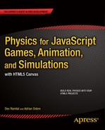
Consider first a special case in which the ball hits the wall perpendicularly with velocity v (see Figure 11-1). In that case, the ball will bounce back at a right angle as well. Therefore, because its velocity magnitude is unchanged, its velocity just after bouncing will be –v.
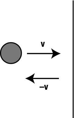
Figure 11-1. A ball bouncing off a wall at a right angle
This is very easy to implement in code: you just reverse the velocity direction after the collision detection. However, there is something else to consider. When collision is detected, the ball may have passed the edge of the wall, penetrating it slightly. Therefore, before you reverse the ball’s velocity, you need to reposition the ball just at the edge of the wall (see Figure 11-2). This is necessary not just to avoid the visual effect of the ball penetrating into the wall but also to avoid the potential problem of the ball “getting stuck” in the wall. The latter situation might arise if the reversed velocity of the ball is not sufficient for it to get out of the wall (especially if the velocity is also reduced to account for energy loss—see the next section). In that case, the velocity of the ball would be reversed again on the next timestep, sending it back into the wall.
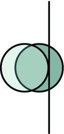
Figure 11-2. Repositioning the ball after collision detection
The following code illustrates these steps for the scenario shown in Figure 11-2, for a Ball instance named ball and a wall object named wall:
if (ball.x > wall.x - ball.radius){  // collision detection
     ball.x = wall.x - ball.radius;  // reposition ball at wall edge
     ball.vx *= -1; // reverse ball’s velocity
}
These simple three lines encapsulate the whole process of handling the bouncing of a ball colliding perpendicularly with a horizontal or vertical wall:
- Collision detection: simple in this case.
- Reposition the particle at the point of collision: in this case, shift it horizontally or vertically so that it just touches the wall.
- Calculate the particle’s new velocity just after the collision: here, for elastic collisions normal (perpendicular) to the wall, just reverse the velocity.
Note that in steps 1 and 2 the preceding code assumes that the ball’s position is taken to be that of its center. If, for instance, the ball’s position is instead taken to be the upper-left corner of its bounding box, then its diameter should be subtracted in the corresponding lines of code. Also, this code covers only the situation where the ball is moving from left to right, but it is not difficult to see how you can modify it to move the ball from right to left instead.
This is all nice and simple, but what if the ball hits the wall at an oblique angle (see Figure 11-3), instead of at a right angle? In that case, in implementing step 3, we need to consider the components of velocity perpendicular and parallel to the wall separately. In the case of a vertical wall shown in Figure 11-3, the perpendicular component is ball.vx, and the parallel component is ball.vy. We need to reverse the perpendicular component as before and leave the parallel component unchanged. This is just what the previous piece of code does, so it should work well for an oblique impact as well. This technique of decomposing the velocity vector into a normal (perpendicular) and a parallel (tangential) component with respect to the wall seems entirely natural in this context. But its application is more general; you’ll see in the next section that a variant of it applies to the collision between two particles.

Figure 11-3. Ball bouncing off a wall at an oblique angle
If you need to be extra accurate, there is something else you need to worry about, this time in relation to step 2. Take a look again at Figure 11-3. In the previous code, we reposition the ball by moving it along the x-direction so that it just touches the wall. But when the collision is oblique, the ball’s real position at the point of collision is along the line of collision. So the ball also needs to be moved a little along the y-direction. We’ll devise a general method to do that in the next section. For this simple example, let’s just adjust the x-position only. This should work fine and produce a smooth bouncing effect in most common situations (except perhaps if you have a slow machine, in which case you might find that the ball occasionally sticks to the wall).
The downloadable file wall-bouncing.js demonstrates this simple example. Here is the code:
var canvas = document.getElementById('canvas'),
var context = canvas.getContext('2d'),
var canvas_bg = document.getElementById('canvas_bg'),
var context_bg = canvas_bg.getContext('2d'),

var ball;
var wallX = 400;
var t0, dt;

window.onload = init;
function init() {
     // create a ball
     ball = new Ball(15,'#000000',1,0,false);
     ball.pos2D = new Vector2D(100,100);
     ball.velo2D = new Vector2D(200,50);
     ball.draw(context);
     // create a wall
     context_bg.strokeStyle = '#333333';
     context_bg.beginPath();
     context_bg.moveTo(wallX,50);
     context_bg.lineTo(wallX,350);
     context_bg.closePath();
     context_bg.stroke();
     // make the ball move
     t0 = new Date().getTime();
     animFrame();
};

function animFrame(){
     animId = requestAnimationFrame(animFrame,canvas);
     onTimer();
}
function onTimer(){
     var t1 = new Date().getTime();
     dt = 0.001*(t1-t0);
     t0 = t1;
     if (dt>0.2) {dt=0;};
     move();
}
function move(){
     moveObject(ball);
     checkBounce(ball);
}
function moveObject(obj){
     obj.pos2D = obj.pos2D.addScaled(obj.velo2D,dt);
     context.clearRect(0, 0, canvas.width, canvas.height);
     obj.draw(context);
}
function checkBounce(obj){
     if (obj.x > wallX - obj.radius){
          obj.x = wallX - obj.radius;
          obj.vx *= -1;
     }
}
As you can see, the code in init() simply creates a ball as a Ball object and draws a straight line to represent a wall. The bulk of the subsequent animation code is familiar. Here we are not imposing any forces. Therefore, the velocity of the ball is constant, except when it collides with the wall. The key functionality is provided by the checkBounce() method, which contains a piece of conditional code identical to the one given previously for a ball colliding perpendicularly with the wall. Note that this code would have to be modified slightly if the wall were on the left side or horizontal. And if the wall were neither horizontal nor vertical, but at some angle, you’d need a lot more code than just those three lines in the checkBounce() method, as you’ll soon find out!
Inelastic bouncing
In the previous example, we assumed that there is no loss of kinetic energy, in other words that the collision is elastic. Doing this means the ball bounces back with the same velocity magnitude. In real-world collisions there is always some loss of kinetic energy. It is very easy to include the effect of loss of kinetic energy due to bouncing. All you have to do is multiply the velocity of the ball normal to the wall by a factor of less than 1 when reversing it.
Hence, in the previous example, the following line:
ball.vx *= -1;
would be replaced by something like this, where vfac is a number between 0 and 1:
ball.vx *= -vfac; // energy loss on bouncing
A value of 1 corresponds to an elastic collision, while a value of 0 corresponds to a completely inelastic collision (discussed in more detail a little later), in which the ball just sticks to the wall. You can experiment with different values of vfac to see what you get.
The reason for multiplying the velocity by this constant factor will become clear later, when we discuss one-dimensional collisions.
Similarly, you can model the effect of wall friction in a simple way by multiplying the tangential velocity of the ball (the velocity component parallel to the wall) by a factor between 0 and 1:
ball.vy *= vfac2; // wall friction
Note the absence of a minus sign in this case, as friction reduces but does not reverse the tangential velocity.
The situation becomes significantly more complicated if the wall on which the ball bounces is inclined at some angle to the horizontal or vertical. The same steps apply as in the case of a horizontal or vertical wall, but they are now a bit more complex to implement. Different approaches could be taken here. One common approach, described in the book Foundation HTML5 Animation with JavaScript, by Billy Lamberta and Keith Peters (Apress, 2011), is to perform a coordinate rotation to make the wall horizontal, do the bouncing, and then rotate the coordinate system back. This is a perfectly good way to do it, and we refer you to that book for details on the procedure. For our present purposes, because we are using vectors, we have devised an alternative method that exploits the vector formulation and avoids the two coordinate rotations. We explain the steps of the new method in detail before giving an example of how to implement it.
Collision detection with an inclined wall
Collision detection is much less straightforward when bouncing off an inclined wall because it is not simply a case of checking the x- or y-position of the ball in relation to that of the wall. But thinking in terms of vectors helps a lot. Take a look at Figure 11-4, which shows a particle approaching collision with a wall. There are basically two conditions that must be met for a collision to occur:
- The perpendicular distance of the particle from the wall must be smaller than its radius.
- The particle must be located between the end points of the wall.
Figure 11-4. A ball approaching a wall
There are a number of ways to implement either condition. We describe one possible approach here. Figure 11-5 shows a diagram of the position and displacement vectors corresponding to the setup in Figure 11-4. In this diagram, p1 and p2 are the position vectors of the end points of the wall with respect to the origin O; w is a vector from the end point marked A (with position vector p1) to the other end point. Similarly, p is the position vector of the ball with respect to the origin, b1 and b2 are vectors from the ball to the end points of the wall, and d is a perpendicular vector from the ball to the wall (so that d is equal to the distance PQ of the ball from the wall). Note that we are taking the position of a particle to be at its center. This is true of any Ball instance created from the Ball object.
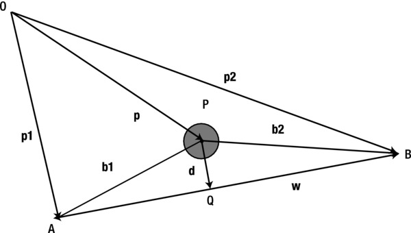
Figure 11-5. Vector diagram for analyzing the collision of a ball with an inclined wall
In terms of these vectors, the first condition is simply the following, where r is the radius of the ball:
![]()
The second condition can be stated in terms of the projections QA and QB of the vectors b1 and b2 in the direction of the wall vector w. If the length of both of those projections is less than the length of w, it means that the ball is between the end points of the wall. Otherwise, if either projection exceeds the length of w, the ball must be outside of that range and won’t hit the wall.
It remains now to work out the length of the projections and the distance d from the known vectors p1, p2, and p. By using the rules of vector addition, we get the following:
![]()
In pseudocode, this is:
wallVec = wall.p2.subtract(wall.p1);
By a similar reasoning, the vectors b1 and b2 are given by these equations:
![]()
![]()
In pseudocode, they can be written as follows:
ballToWall1 = wall.p1.subtract(ball.pos2D);
ballToWall2 = wall.p2.subtract(ball.pos2D);
Then the projection of the vectors ballToWall1 and ballToWall2 onto w is given by this:
proj1 = ballToWall1.projection(wallVec);
proj2 = ballToWall2.projection(wallVec);
The vector d, which we’ll call dist in pseudocode, can then be obtained by subtracting from b1 the projection vector of b1 onto w. In pseudocode it can be written like this:
dist = ballToWall1.subtract(ballToWall1.project(wallVec));
The project() function will be introduced later in the chapter. You can probably express these quantities in a number of different but equivalent ways. We leave that to you as an exercise!
The formula you saw in the previous section for repositioning the particle at collision detection is specific to a vertical wall on the right side in relation to the location of the ball. Its form will look slightly different for the walls on the left, top, or bottom. And it’s no good if the wall is inclined. We need something better. That’s where vectors come to the rescue again. With vector methods, it is possible to come up with a formula that works for any particle velocity and any wall orientation.
Figure 11-6 shows a ball hitting an inclined wall, and the collision being detected after the ball has gone a small distance into the wall. As the diagram indicates, the ball must be moved a distance Δs = h back along its line of approach (opposite to its velocity vector). Here we are assuming that the direction of the velocity vector is constant during that small interval. If a force such as gravity is present, this is not strictly true, but because the time interval is so small, the velocity direction can be taken as constant to a very good approximation.
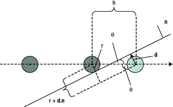
Figure 11-6. Repositioning a particle after collision detection with an inclined wall
Simple trigonometry then shows that the magnitude of Δs is given by the following expression, where d is a perpendicular vector from the particle’s center at the point of collision detection to the wall (so that its magnitude d is the distance of the particle from the wall), n is a unit vector perpendicular to the wall and pointing into the side where the particle normally resides, and θ is the angle between the line of approach of the particle (and therefore its velocity just before collision) and the wall:

Note that if the ball’s center at the point of collision detection lies in front of the wall, then d is opposite to n, and therefore d ∙ n = –d; if it lies behind the wall, then d points along n, and so d ∙ n = d. Using the dot product automatically handles both cases.
In pseudocode, the displacement vector to reposition the particle is then given by this:
displ = particle.velo2D.para(deltaS);
Therefore, the particle’s position needs to be updated as follows:
particle.pos2D = particle.pos2D.subtract(displ);
This all looks nice and simple in comparison to the use of special non-vector code for each wall.
Just as it is with a horizontal or vertical wall, the particle’s new velocity after bouncing is calculated by first decomposing the velocity before bouncing into components parallel and normal to the wall, and then reversing the normal component. But because the wall is now oblique, those components are not just the vx and vy properties of the particle. Instead, we have to specify them as Vector2D objects in their own right.
See Figure 11-7 for an illustration of how to do this. If d is a vector from the particle center normal to the wall at the point of collision, the normal velocity is given as a vector with magnitude equal to the projection of the particle’s velocity onto d and in the same direction as d.
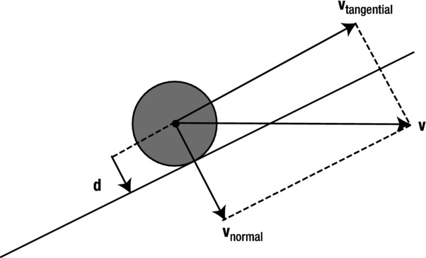
Figure 11-7. Decomposing the velocity vector
In pseudocode, if we calculate the perpendicular vector from the particle to the wall as dist and denote the particle as particle, the normal velocity is given by the following using the projection() and para() methods of the Vector2D object:
normalVelo = dist.para(particle.velo2D.projection(dist));
Recall that vec1.projection(vec2) gives the length of the projection of vector vec1 in the direction of vec2, and that vec.para(mag) gives a vector parallel to vector vec and of length mag.
We can make the code even simpler by creating the following project() method in the Vector2D object:
function project(vec) {
     return vec.para(this.projection(vec));
}
Thus, vec1.project(vec2) gives a vector in the direction of vector vec2 and with magnitude equal to the projection of vec1 in the direction of vec2. With this newly defined method, we can write the normal velocity simply as follows:
normalVelo = particle.velo2D.project(dist);
The tangential velocity can then be obtained simply by subtracting the normal velocity from the particle velocity (see Figure 11-7):
tangentVelo = particle.velo2D.subtract(normalVelo);
These are the precollision velocities. Assuming there is no energy loss, the collision will reverse the normal velocity while leaving the tangential velocity unchanged. Therefore, the new velocity of the particle as a result of the collision is given by this:
particle.velo2D = tangentVelo.addScaled(normalVelo,-1);
If there is energy loss due to bouncing, simply replace the –1 in the previous code by the fraction vfac discussed in the previous section.
Velocity correction just before collision
If you are creating a simulation that involves a force, such as gravity, there is something else to worry about. Whenever there is a force involved, it means that the particle is accelerating (its velocity is changing all the time). In that case, when the particle is repositioned at the edge of the wall, its velocity must also be adjusted to what it was at that point. Although this may seem like a small correction, failure to do so could in some cases result in serious loss of accuracy. This applies equally to horizontal or vertical walls if the velocity is changing with time.
Let’s consider a simple example: a ball dropped from a certain height onto a horizontal floor. Suppose that collision is detected when the ball has gone slightly past the floor level. If you simply follow the procedure given so far, you would move the ball to the level of the floor and then reverse its velocity (if you assume no energy loss due to bouncing). The trouble is that because the ball is accelerating under gravity, its velocity at the point of collision detection is higher than it should be at the actual point of collision. By simply reversing this velocity, you are sending it off with higher kinetic energy than it’s supposed to have as a result of having lost potential energy by falling from its initial height. The consequence is that the ball will end up reaching higher than the point it fell from! After a few bounces, the animation could become completely unstable. Of course, if you implement energy loss on bouncing, you may not even notice the problem—if accuracy is not important, that may be a simple trick to solve the problem. But if you want to be as accurate as possible, or if the nature of the simulation does not permit you to include energy loss, then here is the way to do it.
The aim is to compute the velocity of the particle at the point of collision given that it is accelerating. We know the velocity, acceleration, and displacement at the point of collision detection. To proceed, let’s start with the calculus definition of acceleration:

For a reason that will become apparent shortly, we can write it as the following (you can think of the two ds factors as “cancelling out”):

Now, because v = ds/dt, we can write it as follows:

This gives us a differential equation connecting the quantities that we were just talking about. Because we are doing a discrete simulation, let’s write this:

Substituting into the preceding equation gives this:

And so:

This formula gives the change in velocity Δv that results from a displacement Δs under an acceleration a. Let v be the velocity at collision detection and v’ be the velocity at collision, so that:
![]()
Simple algebra gives this:
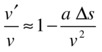
This formula gives the ratio of the magnitude of the velocity at the point of collision to that at the point of collision detection in terms of the acceleration (which is constant in the case of gravity), the velocity at the point of collision detection, and the displacement of the particle from the point of collision to the position where collision is detected. The latter quantity was worked out in the section “Repositioning the particle.” Therefore, the adjustment factor for the velocity can be calculated from these known quantities as given by the preceding formula. The formula was derived for a 1D case because we didn’t use vectors, but it applies equally to 2D when the acceleration a and the displacement Δs are vectors that may not be in the same direction (for example, for a ball moving under gravity). In that case, we take the acceleration resolved in the direction of the displacement, so that in effect we need to replace the product aΔs by the dot product a.Δs; and v is the magnitude of the velocity vector.
Let’s denote the code variable corresponding to the velocity correction factor v’/v as vcor. Then, assuming that the direction of the velocity does not change much between the point of collision and the point of collision detection, we can write this in pseudocode:
veloAtCollision = veloAtCollisionDetection.multiply(vcor);Example: a ball bouncing off an inclined wall
All that vector algebra we’ve been discussing is probably beginning to sound a bit heavy. So it’s time to pull together all you have learned in this section to build a full example. Because we are going to do a lot of bouncing around walls, it would make sense to create a reusable Wall object. Let’s do that first.
The Wall object is a simple object that draws a line between two specified end points to represent a wall. The end points are Vector2D objects. Here is the full code of the Wall object:
function Wall(p1,p2){
     this.p1 = p1;
     this.p2 = p2;
     this.side = 1;
}
Wall.prototype = {
     get dir (){
          return this.p2.subtract(this.p1);
     },
     get normal (){
          return this.dir.perp(1);
     },
     draw: function (context) {
          context.save();
          context.strokeStyle = '#000000';
          context.lineWidth = 1;
          context.beginPath();
          context.moveTo(this.p1.x,this.p1.y);
          context.lineTo(this.p2.x,this.p2.y);
          context.closePath();
          context.stroke();
          context.restore();
     }
}
The end points, denoted by p1 and p2, are supplied as arguments in Wall’s constructor. Properties wall.dir and wall.normal are defined via getters that return the vector from p1 to p2 (the vector along the wall) and the unit vector normal to the wall, respectively. The usefulness of these properties will soon become apparent. The side property will be discussed in the section “Dealing with a potential ‘tunneling’ problem.”
In the file wall-object.js, we demonstrate how to create a Wall instance that is at an oblique angle to the horizontal by the following piece of code:
var p1 = new Vector2D(100,200);
var p2 = new Vector2D(250,400);
var wall = new Wall(p1,p2);
wall.draw(context);
So the end point vectors p1 and p2 are [100, 200] and [250, 400], respectively.
Getting a ball to bounce off an inclined wall
In the bouncing-off-inclined-wall.js file we first create a ball and an inclined wall and then make the ball move under gravity onto the wall (see Figure 11-9 later in the chapter) using the usual animation code with a gravity force Forces.constantGravity in calcForce(). The move() method adds a new method, checkBounce(), which looks as follows:
function checkBounce(obj){
     // vector along wall
     var wdir = wall.dir;
     // vectors from ball to endpoints of wall
     var ballp1 = wall.p1.subtract(obj.pos2D);
     var ballp2 = wall.p2.subtract(obj.pos2D);
     // projection of above vectors onto wall vector
     var proj1 = ballp1.projection(wdir);
     var proj2 = ballp2.projection(wdir);
     // perpendicular distance vector from the object to the wall
     var dist = ballp1.addScaled(wdir.unit(), proj1*(-1));
     // collision detection
     var test = ((Math.abs(proj1) < wdir.length()) && (Math.abs(proj2) < wdir.length()));
     if ((dist.length() < obj.radius) &&  test){
          // angle between velocity and wall
          var angle = Vector2D.angleBetween(obj.velo2D, wdir);
          // reposition object
          var normal = wall.normal;
          if (normal.dotProduct(obj.velo2D) > 0){
               normal.scaleBy(-1);
          }
          var deltaS = (obj.radius+dist.dotProduct(normal))/Math.sin(angle);
          var displ = obj.velo2D.para(deltaS);
          obj.pos2D = obj.pos2D.subtract(displ);
          // velocity correction factor
          var vcor = 1-acc.dotProduct(displ)/obj.velo2D.lengthSquared();
          // corrected velocity vector just before impact
          var Velo = obj.velo2D.multiply(vcor);
          // velocity vector component perpendicular to wall just before impact
          var normalVelo = dist.para(Velo.projection(dist));
          // velocity vector component parallel to wall; unchanged by impact
          var tangentVelo = Velo.subtract(normalVelo);
          // velocity vector component perpendicular to wall just after impact
          obj.velo2D = tangentVelo.addScaled(normalVelo,-vfac);
     }
     // collision at the wall boundaries
     else if (Math.abs(ballp1.length()) < obj.radius){
          bounceOffEndpoint(obj,wall.p1);
     }
     else if (Math.abs(ballp2.length()) < obj.radius){
          bounceOffEndpoint(obj,wall.p2);
     }
}
This code closely mirrors the description given in the previous sections. Most of it should therefore be straightforward (and we’ve left the comments in so you can follow the logic more easily). Let’s therefore focus on just a couple of features that were not covered in the preceding discussion.
First, in the code that repositions the ball after collision detection, note that we check whether the wall normal vector has a positive dot product with the ball’s velocity vector; if so, we reverse the wall normal vector. To understand why this is done, refer to the section “Repositioning the particle,” in which we said that the normal must point to the side where the particle resides. The latter condition is equivalent to saying that the normal vector should point so that it has a normal component in the opposite direction to the ball’s velocity and so should have a negative dot product with it (see Figure 11-8). The if code enforces that condition. But why do we need to check this every timestep; can’t we fix the normal once and for all? The reason is that by doing so we allow for the possibility that the ball could bounce on the bottom surface as well as on the top surface of the wall.
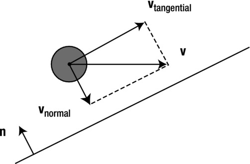
Figure 11-8. The unit normal vector to the wall should be oriented opposite to the velocity vector
The second thing to point out is the presence of the two else if blocks at the end of the checkBounce() function. They are there to handle the case where the ball is within a radius of either of the end points of the wall. In that case, they call a new method: bounceOffEndpoint(). The idea is that bouncing off the edge of the wall should give rise to a different type of motion and should therefore be handled differently. The approach we take is to handle such a collision in a similar way to that between two particles, with the additional feature that here one of the “particles,” the wall end point, is fixed and has zero radius. The code within the bounceOffEndpoint() method probably won’t make too much sense now, but it should once you’ve covered the material on collisions between particles later in the chapter.
To make the simulation more interactive and fun, there is also code that allows you to click and drag anywhere on the canvas to change the position and size of the ball. On releasing the mouse, the simulation resumes with the new ball.
Spend some time experimenting with the simulation. Click and drag to create balls of different sizes and see how they fall and bounce onto the inclined wall in a natural way. Avoid overlapping the ball with the wall when you are dragging as this will result in erratic behavior. Release the ball onto the end points of the wall and notice the difference in the way it bounces. Change gravity g and the energy loss factor vfac. See Figure 11-9 for a screenshot of the simulation.
Figure 11-9. A ball bouncing off an inclined wall
Next release the ball just above the line, so that it starts to slide down the wall. You might find that the ball tends to get “stuck” if it just slides without bouncing. The problem is that our code handles collision resolution but not contact resolution. To fake contact resolution, you can cheat by introducing the following line in checkBounce(), just after the ball’s position vector pos2D is updated:
obj.y -= 0.1;
This raises the ball very slightly (by just 0.1 px) above the wall each time it comes into contact with it. The result is that the ball then falls back onto the wall again, experiencing a series of consecutive collisions as it slides down the wall. Run the simulation again with this additional line, and see how the ball now slides down the wall, apparently smoothly. This is strongly reminiscent of the simulation of a ball sliding down an inclined plane that we did back in Chapter 7 using normal contact forces. In fact, this is a common approach to handling contact resolution: using impulses produced by “micro-collisions” rather than by explicitly including a normal contact force.
Dealing with a potential “tunneling” problem
The method of collision detection we described in the previous section and implemented in this simulation should work well under most normal circumstances. But in some cases, especially if the simulation is run on a slow machine and the ball is small and moving fast, it may be possible for the ball to cross the wall completely in a single timestep. In that case, collision detection will fail. This is known as tunneling. You can probably see this effect if you make the ball very small (1 px) and release it a long way above the wall so it achieves a high velocity by the time it hits the wall. The ball might then pass straight through the wall.
The collision detection algorithm outlined in the previous section fails because the first condition (that the particle is closer to the wall than its radius) is never satisfied. We need to modify the algorithm to include the new possible scenario. A simple solution is to test whether the ball’s center has moved from one side of the wall to the other. If so, that means it has “tunneled,” and that in itself provides the collision detection.
We have implemented this collision detection mechanism in a modified version of the simulation with source files bouncing-off-inclined-wall2.js. If you compare this modified code with the original, you will find that a key change is the inclusion of the new checkSide() and setSide() methods in the init() and onUp() methods:
function checkSide(){
     var wdir = wall.dir;
     var ballp1 = wall.p1.subtract(ball.pos2D);
     var proj1 = ballp1.projection(wdir);
     var dist = ballp1.addScaled(wdir.unit(), proj1*(-1));
     setSide(dist);
}
function setSide(dist){
     if (dist.dotProduct(wall.normal) > 0){
          wall.side = 1;
     }else{
          wall.side = -1;
     }
}
The setSide() method is also called in checkBounce(). This code provides a way to keep track of which side of each wall the ball is at any moment. To do this, it checks the sign of the dot product between the perpendicular vector dist from the particle to the wall and the wall normal vector. If the sign is negative, it sets the side property of the wall to –1; otherwise, it sets it to 1. The side property of the Wall object has been created specifically for this purpose.
Another important new piece of code in checkBounce() checks to see whether the sign of the dot product has reversed (which means the ball has tunneled); if so, it sets the testTunneling Boolean variable to true:
var testTunneling;
if (wall.side*dist.dotProduct(wall.normal) < 0){
     testTunneling = true;
}else{
     testTunneling = false;
}
The value of testTunneling is then used as part of the collision detection test:
if (( (dist.length() < obj.radius) || (testTunneling) ) &&  test){
     ...
}
This sets up the basic collision detection in the case of tunneling. The rest of the changes in the code should be easy to follow.
If you test bouncing-off-inclined-wall2.js you should find that the tunneling problem is fixed.
Example: Ball bouncing off multiple inclined walls
In bouncing-off-multiple-inclined-walls.js we generalize the preceding simulation to include several walls (see Figure 11-10). Take a look at the source files; the code extends the previous example in a straightforward way. First, you just add more walls in init() in the same way—four inclined walls, plus four bounding walls to form a box that encloses the other walls and the ball. The checkBounce() method now loops over each wall. It also includes a new hasHitAWall Boolean variable that is used to stop the looping once a collision with one of the walls is detected.
Figure 11-10. Ball bouncing off multiple walls
Experiment with the simulation, remembering that you can click and drag to reposition and resize the ball. As before, avoid positioning the ball so that it overlaps with any of the walls. Doing so will introduce an unphysical initial condition (a ball cannot physically overlap with a wall) that will cause some of the equations to give nonsensical results, resulting in erratic and unpredictable behavior.
See how the simulation handles different scenarios properly. For example, try balls of different sizes and release them at different locations: above the walls, so that they bounce off; just on the walls, so that they slide down; or just above a gap between the walls too small for them, so that they get trapped. You will see that collisions under the walls are also handled properly. Note that the four confining walls are treated in exactly the same way as the others. You can also click and drag above the top wall to make the ball bounce off it!
As in the previous simulation, you may encounter the tunneling problem on a slower machine. To fix this, we have modified the simulation in exactly the same way as described in the previous subsection. The modified source code is in the files bouncing-off-multiple-inclined-walls2.js. You might find that tunneling still sometimes happens at very high velocities (for example, try initializing the ball’s velocity with a magnitude in excess of 1000 px/s). The problem there is that we are at the limit of the time resolution of the simulation, which is limited by how fast your machine can run it.
Collisions between particles in 1D
In this section, we will show you how to handle collisions between particles when the approach direction of the particles lies along the line joining them. This situation can be described as a 1D collision because the motion of the particles takes place in a straight line, both before and after the collision. In general, two particles may collide at any angle, changing their direction as they do so. Therefore, the case discussed in this section may seem like a very special case. So why study it? The reason is that the methods and formulas that hold in this special case can be readily extended to the more general case where the particles may collide at any angle. In fact, we will do that in the next section.
The steps for handling 1D particle collisions are the following (mirroring the steps for resolving the bouncing of a particle moving perpendicular to a wall):
- Collision detection
- Repositioning the particles at the moment of collision
- Calculating the new velocities just after the collision
In the case of spherical particles (or circular in 2D), the first step, collision detection, is very simple. As discussed in Chapter 2, you just see whether the distance d between the centers of the two particles is less than the sum of their radii, where d is calculated from the position coordinates (x1, y1) and (x2, y2) using the Pythagorean theorem:
![]()
In 2D:
![]()
Let’s now look at how to reposition the particles when a collision is detected.
Just as a particle may sink some distance into a wall by the time a collision is detected, two particles may similarly overlap. The complication in this case is that in general both particles may be moving, so both need to be moved back to their position at the actual point of contact. But how do we know how much to move each particle?
Let’s begin by considering the case when the two particles are moving toward each other, as shown in Figure 11-11.
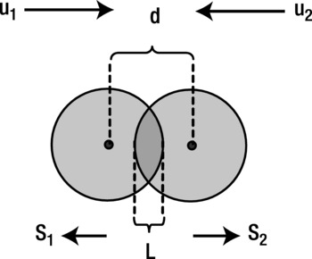
Figure 11-11. Separating overlapping particles moving toward each other
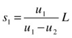
The amount of overlap L is given by the following, where r1 and r2 are the radii of the two particles, and d is the distance between their centers, as given by the Pythagorean formula discussed in the previous section:
![]()
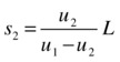
Let s1 and s2 be the magnitudes of the displacements by which the particles must be moved, in opposite directions, so that they are just touching. These displacements must add up to give the overlap distance L:
![]()
This gives one equation relating s1 and s2 in terms of a known variable L. In order to be able to work out s1 and s2, we need a second equation connecting them. We can come up with such an equation by recalling that, in a small time interval t:
![]()
and
![]()
where u1 and u2 are the velocities of the respective particles just before the collision. That’s just using the fact that displacement = velocity × time (see Chapter 4).
Dividing the first equation by the second gives this:

This is our second equation. It is now a matter of simple algebra to solve for s1 and s2 to give this:
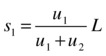
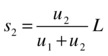
What this result tells us is that the particles must be displaced in proportion to their velocities just before the impact.
This is great, but what if we have the other possible situation, in which the two particles are moving in the same direction (rather than toward each other) with the one behind moving faster (so that a collision actually happens), as shown in Figure 11-12.
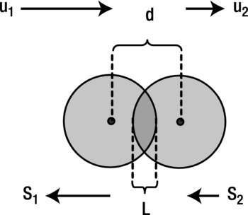
Figure 11-12. Overlapping particles moving in the same direction
In that case, the first equation connecting the displacement magnitudes s1 and s2 becomes the following, while the second equation is unchanged:
![]()
Solving them simultaneously then gives this:
and this:
This is a bit messy because we have different equations depending on whether the particles are moving toward each other or not. Luckily, it is possible to incorporate both cases into a single solution by thinking in terms of vector displacements. The reasoning is slightly less intuitive, but here is the final result, where the symbol |v| signifies the magnitude of vector v:
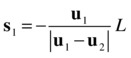
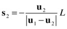
Note that we always divide by the magnitude of the relative velocity (u1 – u2). When the particles are approaching each other, this is (u1 + u2); otherwise, it is (u1 – u2). Hence, these equations indeed reduce to the corresponding equations for the displacement magnitudes in the two cases discussed previously. The other good thing is that here the direction of the displacements is also explicit in the formulas: the minus sign tells us that s1 is opposite to u1, and s2 is opposite to u2.
You now know how to reposition the particles once the collision is detected. The final thing to do is to calculate the new velocities of the colliding particles just after the collision. We’ll do this separately for elastic and inelastic collisions.
Recall from Chapter 4 that an elastic collision is one in which kinetic energy is conserved. This means we can apply conservation of kinetic energy in addition to conservation of momentum (which is always conserved in any collision, elastic or not). For example, the collisions between billiard balls are usually modeled as elastic collisions.
Let the two colliding particles (which we can call particle1 and particle2) have masses m1 and m2, initial velocities u1 and u2, and final velocities v1 and v2, respectively. Note that we need only one component of velocity because the motion is 1D. Then we can write momentum conservation and energy conservation as follows:
![]()
![]()
Here the masses m1 and m2 of the particles are known, and so are the initial velocities u1 and u2. The aim is to calculate the final velocities v1 and v2 in terms of these known variables. This is a matter of solving these two equations simultaneously. The easiest method to do so involves deriving an important intermediate result involving the relative velocities of the particles before and after the collision. So let’s do that now.
Relative velocity of colliding particles
The first step in deriving the relative velocity of the colliding particles is to rearrange the previous two equations by combining the terms for each particle on each side of the equation (put all the terms with a 1 subscript on one side and the terms with a 2 subscript on the other side):
![]()
![]()
Now recall the following identity from your school algebra:
![]()
This allows you to write the second equation as follows:
![]()
You can now see that each side of this equation contains the corresponding side of the first equation as a factor. So you can divide this equation by the first equation to get rid of those factors, leaving us with this:
![]()
This can be rearranged by combining the initial velocities (the u variables) on one side and the final velocities (the v variables) on the other side of the equation to give this:
![]()
Or, equivalently, this:
![]()
This is our result. Note that (u1 – u2) is the initial relative velocity of particle1 from the point of view of particle2. Similarly, (v1 – v2) is the final relative velocity of particle1 from the point of view of particle2. Therefore, the preceding result tells us that the relative velocity of separation of the two particles is the negative of their relative velocity of approach. This result does not depend on the masses of the particles, because m1 and m2 were cancelled out. But note that it holds only for elastic collisions. We shall see in the next section how it is modified for inelastic collisions.
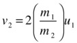
As an immediate application of this result, consider the case when one of the particles, say particle2, is immovable (such as a wall). This is the same as saying that u2 = v2 = 0. Putting these values into the last equation gives us this:
![]()
This is elastic bouncing off an immovable object, and is the condition that we applied in the first example of a ball bouncing elastically off a wall.
Calculating velocities after an elastic collision
Using the result derived in the preceding section, it is now easy to work out the velocities of the particles after an elastic collision. The logic is that energy conservation is incorporated into the equation for relative velocities:
![]()
So we need to solve this equation simultaneously with the equation expressing momentum conservation:
![]()
The goal is to find the final velocities, v1 and v2, in terms of the other variables (the initial velocities and the masses). This can be done by eliminating either v1 or v2 between the two equations and then rearranging the resulting equation to find the other one. For example, we first multiply the first equation by m2 to give this:
![]()
Adding this to the second equation then gets rid of v2, giving this:
![]()
Dividing by (m1+m2) then gives the final result for the velocity of particle1:
You could go through a similar algebraic manipulation to calculate v2, but there is no need to: you can just swap the 1 and 2 indices on the last equation to give this:

This is the result you are after: you can now calculate the velocities of the two particles just after the impact, from the velocities just before the impact (and the masses of the particles).
Finally, note that you don’t have to calculate v2 from the second equation. Once you know v1, you can just work out v2 by rearranging the equation for relative velocities to give the following, which saves on CPU time:
![]()
A special case: particles of equal masses
In the special case of particles that have the same mass, the formulas for their velocities after collision take a particularly simple form. To see this, simply replacing m1 = m2 = m into the preceding equations gives this:
![]()
and this:
![]()
In other words, the particles simply exchange velocities after the collision! This applies regardless of the initial velocities of the particles, as long as they have the same mass and the collision is elastic. This is a very useful result. If your simulation will only ever involve elastic collisions between particles of the same mass, there is no need to code in the complicated general formula given previously, saving on valuable CPU time. You might recall that we made use of this result in the simple collision example in Chapter 5.
As a special case of this special case, if one of the particles is initially at rest (u2 = 0), we get v1 = 0 and v2 = u1; the other particle then stops dead in its track after the collision, while the initially stationary particle moves off at the velocity that the other one had before the collision.
Another special case: collision with a particle of much larger mass
On the other hand, if the mass of one of the particles is much larger than the other (for example, m2 >> m1), the formulas for the final velocities reduce to this:
![]()
and this:

In particular, if the particle with large mass (particle2) is initially stationary, u2 = 0, so
![]()
and
Hence, the lighter particle bounces off the heavier one, almost reversing its velocity. Noting that (m1/m2) is a small number much less than 1, we conclude that v2 << u1; hence, the heavier particle moves off at a much smaller velocity than the velocity at which the first particle hit it. This is all common sense.
Although it is common to model collisions as elastic, most collisions in real life are rarely elastic—they usually involve a loss of kinetic energy and are therefore inelastic.
To model inelastic collisions, a useful starting point is again the relative velocity of the colliding particles—through the introduction of a concept known as the coefficient of restitution.
Coefficient of restitution
The coefficient of restitution (denoted by the symbol CR) is defined as the ratio between the relative velocity after a collision and the relative velocity before the collision:.
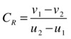
This equation can be rewritten as follows:
![]()
For an elastic collision, the relative velocities before and after the collision are related by the equation ![]() , so the preceding equation tells us that CR = 1 for an elastic collision.
, so the preceding equation tells us that CR = 1 for an elastic collision.
Conceptually, the coefficient of restitution is a measure of the departure from perfectly elastic collisions. Generally, the value of CR will be less than 1. Collisions for which CR > 1 are also possible; they correspond to collisions that generate explosive forces, so that the total kinetic energy of the particles after the collision is larger than their initial kinetic energy. Such collisions are called superelastic.
The special case when CR = 0 refers to so-called completely inelastic collisions. In that case, the relative velocity equation reduces to this:
![]()
So that:
![]()
In other words, the final velocities of the particles are the same: they stick together. In a completely inelastic collision, the loss of kinetic energy is maximum, but not complete (if it were complete, the particles would just stop; this would violate momentum conservation).
As another special case, suppose that one of the particles is immovable (such as a wall). For example, if particle2 is immovable, u2 = v2 = 0, so that the relative velocity equation gives this:
![]()
This is exactly how we modeled wall collisions involving energy loss earlier in this chapter, with CR representing the “bounce” factor.
Calculating velocities after an inelastic collision
Starting from the relative velocity equation for inelastic collisions and using a method similar to that used to derive the corresponding elastic collision equations, it is easy to show that the final velocities due to an inelastic collision are given by this:
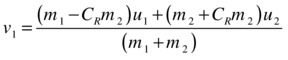
and this:
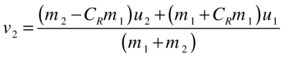
This is the most general formula for collisions, as it also includes the elastic formula as a special case (set CR = 1 in the above formulas and verify that they reduce to the corresponding formulas for elastic collisions).
Completely inelastic collisions
If the collision of two particles is completely inelastic (with CR = 0), the last equations reduce to this:
So the two particles stick together and move at the same velocity after the collision. Examples in which you might want to model completely inelastic collisions include hitting a character with a snowball or firing a bullet that sticks into its target.
This completes our discussion of particle collisions in 1D. You are no doubt eager to see all that math applied in a demo. You’ll get to see a code example very soon, but before we do that, let’s quickly discuss how this extends to 2D. Once we’ve covered that, we will then be able to build simulations that can handle both 1D and 2D collisions.
Collisions between particles in 2D
We are now ready to look at general 2D collisions, in which the direction of approach of the particles is not necessarily along the line joining their centers. The way to handle such collisions is to resort to a trick similar to that used for a ball colliding with a wall: at the point of collision (when the particles are just touching), resolve the velocity of each particle into a normal component along the line joining them, and a tangential component perpendicular to that line (see Figure 11-13). The revelation is that, just as in a collision with a wall, only the normal velocity components are affected by the collision; the tangential components remain the same after the collision (provided it is frictionless). What’s more, the normal velocity components are changed in exactly the same way as if the collision were in 1D (as if the tangential components were zero). That’s great; it means that we can treat any 2D collision as a 1D collision in terms of the normal velocity components.
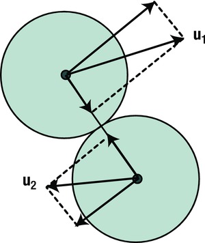
Figure 11-13. Resolving velocity normal and parallel to line joining particles
So the steps for handling 2D particle collisions are the following:
- Detecting the collision
- Decomposing the initial velocities in normal and tangential components
- Repositioning the particles at the moment of collision
- Calculating the new normal velocities just after the collision
- Adding the new normal velocity components back to the tangential components
Compared with the procedure for handling 1D collisions, the extra steps are steps 2 and 5. Note also that, in step 3, the particles are repositioned using the same formula we derived for 1D collisions (see the section “Repositioning the particles”), but using the normal velocities.
As mentioned in the section “Bouncing off inclined walls,” the usual method we found that people use to handle 2D collisions is to rotate the coordinate system, perform a 1D collision, and then rotate back the coordinate system. But armed with vectors, the method we suggest actually proves simpler: in place of coordinate rotations, we simply resolve vectors and later add them up again. Let’s see the method in action!
Example: 2D collisions between two particles
We will create a simulation that can handle a general 2D collision between two particles. Obviously, it will also be able to handle 1D collisions simply by choosing appropriate initial positions and velocities for the particles. This example will pull together everything we have covered on collisions between particles.
Creating a two-particle collision simulator
The code for creating this two-particle collision simulator example is in the file ball-collision.js. The init() method creates the two particles as Ball instances and sets their initial sizes, masses, positions, and velocities before invoking the animation code:
function init() {
     // create a ball
     ball1 = new Ball(15,'#ff0000',1,0,true);
     ball1.pos2D = new Vector2D(0,200);
     ball1.velo2D = new Vector2D(250,0);
     ball1.draw(context);
     ball2 = new Ball(75,'#0000ff',125,0,true);
     ball2.pos2D = new Vector2D(300,200);
     ball2.velo2D = new Vector2D(50,0);
     ball2.draw(context);
     // make the ball move
     t0 = new Date().getTime();
     animFrame();
}
We are creating a small ball of radius 15 pixels and 1 mass unit and a large ball of radius 75 pixels and 125 mass units. Note that we’ve scaled masses on the cube of the radius, based on 3D geometry (recall that the volume of a sphere = 4πr3/3), and assuming that the two balls have the same density (recall that mass = density × volume). On this basis, because the large ball has a radius 5 times that of the smaller one, its mass should be 125 times larger.
In the animation part of the code, the move() method moves each ball in turn and then checks for collision at each timestep:
function move(){
     context.clearRect(0, 0, canvas.width, canvas.height);
     moveObject(ball1);
     moveObject(ball2);
     checkCollision();
}
The checkCollision() method looks like this:
function checkCollision(){
var dist = ball1.pos2D.subtract(ball2.pos2D);
if (dist.length() < (ball1.radius + ball2.radius) ) {
// normal velocity vectors just before the impact
var normalVelo1 = ball1.velo2D.project(dist);
var normalVelo2 = ball2.velo2D.project(dist);
// tangential velocity vectors
var tangentVelo1 = ball1.velo2D.subtract(normalVelo1);
var tangentVelo2 = ball2.velo2D.subtract(normalVelo2);
// move particles so that they just touch
var L = ball1.radius + ball2.radius-dist.length();
var vrel = normalVelo1.subtract(normalVelo2).length();
ball1.pos2D = ball1.pos2D.addScaled(normalVelo1,-L/vrel);
ball2.pos2D = ball2.pos2D.addScaled(normalVelo2,-L/vrel);
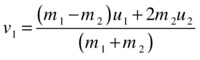
// normal velocity components after the impact
var m1 = ball1.mass;
var m2 = ball2.mass;
var u1 = normalVelo1.projection(dist);
var u2 = normalVelo2.projection(dist);
var v1 = ((m1-m2)*u1+2*m2*u2)/(m1+m2);
var v2 = ((m2-m1)*u2+2*m1*u1)/(m1+m2);
// normal velocity vectors after collision
normalVelo1 = dist.para(v1);
normalVelo2 = dist.para(v2);
// final velocity vectors after collision
ball1.velo2D = normalVelo1.add(tangentVelo1);
ball2.velo2D = normalVelo2.add(tangentVelo2);
}
}
The code follows the explanations given in the previous subsections closely, and the comments in the code should make it clear what is going on at each step. In fact, this code is substantially simpler than the corresponding code for bouncing off an oblique wall. Notice also the symmetry with respect to the two balls. The simplicity and relative brevity of the code provide what we think is an attractive alternative to the usual method of rotating the coordinate system to resolve oblique collisions.
Finally, the formula for calculating the final velocities assumes elastic collisions, but it is a simple matter to replace it with the alternative (and more general) formula for inelastic collisions. We leave this as an exercise for you.
Experimenting with the particle collision simulation
If you run the particle collision simulation, you’ll see the small ball in a 1D collision with the larger one (see Figure 11-14). Let’s start experimenting by verifying some of the observations we made when discussing special cases in 1D elastic collisions.
Figure 11-14. A two-particle collision simulator
First, set the initial velocity of the large one to zero, simply by commenting out the line that sets its velocity in ball-collision.js. You will see that the small ball almost reverses its velocity after the collision, while the larger one moves off with a very small velocity, just as we said before.
Next, make the second ball the same size and mass as the first by replacing the line that instantiates it with the following modified line:
var ball2 = new Ball(15,'#0000ff',1,0,true);
Keep the second ball’s velocity at zero and run the code. You will see that, upon collision, the first ball stops right in its track, while the second ball moves off at the initial velocity of the first ball. Again this confirms the deductions we made previously on the basis of the governing collision equations.
This is a full 2D collision simulator, so why not get the balls to collide at an angle? For example, while keeping the masses and the sizes of the two particles the same, try the following:
ball1.velo2D = new Vector2D(100,-30);
ball2.velo2D = new Vector2D(-50,-30);
This shows that our basic 2D particle collision simulator can handle both 1D and 2D collisions properly. So let’s now add a bit more complexity.
Example: multiple particle collisions
Extending the preceding simulation to handle a large number of particles is simply a matter of creating more ball instances and then checking for collisions between each pair of particles. In multiple-ball-collision.js, we create nine particles of the same size and mass, and animate each one in the move() method, which looks like this:
function move(){
     context.clearRect(0, 0, canvas.width, canvas.height);
     for (var i=0; i<numBalls; i++){
          var ball = balls[i];
          moveObject(ball);
     }
     checkCollision();
}
The checkCollision() method is very similar to the two-particle version in ball-collision.js, the main difference being a double for loop in the present version:
function checkCollision(){
     for (var i=0; i<balls.length; i++){
          var ball1 = balls[i];
          for(var j=i+1; j<balls.length; j++){
               var ball2 = balls[j];
                        //code in here is similar to ball-collision.js
                }
        }
}
The key task with the for loops is to pick all possible pairs of particles without double-counting. So the first loop iterates over all the elements of the balls array, picking the first ball, ball1, from it. The second loop then iterates over the elements of balls again to pick ball2, but this time starting from the next element from ball1. This avoids checking for collisions between ball1 and ball2, and then again between ball2 and ball1.
The nine balls are initially positioned randomly on the canvas. They are given velocities toward the center of the canvas, with a velocity magnitude proportional to their distance from the center. When you run the simulation, the balls move to the center, where they collide a number of times in quick succession, as a result of which they bounce outward. Feel free to experiment with different configurations and initial velocities.
Example: multiple particle collisions with bouncing
The previous example was interesting, but the particles only collided briefly before separating and disappearing outside the canvas area. It would be much more fun to confine them so that they collide over and over again. To do this, we need to introduce confining walls. So, let’s combine everything we have learned in this chapter and build one final example involving multiple particles colliding with each other and with walls. The particles will also have different sizes and masses.
We call the new file molecules.js because the result will look like gas molecules bouncing about. Here is the init() method in molecules.js:
function init() {
     balls = new Array();
     for(var i = 0; i < numBalls; i++){
          var radius = Math.random()*20 + 5;
          var mass = 0.01*Math.pow(radius,3);
          var ball = new Ball(radius,'#666600',mass,0,true);
          ball.pos2D = new Vector2D(Math.random()*(canvas.width-2*radius)+radius, Math.random()*(canvas.height-2*radius)+radius);
          ball.velo2D = new Vector2D(((Math.random()-0.5)*100),((Math.random()-0.5)*100));
          balls.push(ball);
          ball.draw(context);
     }
     walls = new Array();
     var wall1 = new Wall(new Vector2D(canvas.width,0),new Vector2D(0,0));
     wall1.draw(context_bg);
     walls.push(wall1);
     var wall2 = new Wall(new Vector2D(canvas.width,canvas.height),new Vector2D(canvas.width,0));
     wall2.draw(context_bg);
     walls.push(wall2);
     var wall3 = new Wall(new Vector2D(0,canvas.height), new Vector2D(canvas.width,canvas.height));
     wall3.draw(context_bg);
     walls.push(wall3);
     var wall4 = new Wall(new Vector2D(0,0),new Vector2D(0,canvas.height));
     wall4.draw(context_bg);
     walls.push(wall4);
     t0 = new Date().getTime();
     animFrame();
}
We first create a set of balls with random radius ranging from 5 px to 25 px, and with masses proportional to the cube of the radius. The balls are positioned randomly on the canvas and given random velocities with a maximum magnitude of 50 px/s. Then four walls are created at the edges of the canvas. The animation code is then called.
The rest of the code is basically a hybrid of the codes used for multiple colliding particles (the previous example) and for bouncing off multiple walls. Hence, there is nothing substantially new, except in the way they are combined. The move() method is identical to that in the previous example with multiple colliding particles. The checkCollision() method is almost identical with that of the previous example, except for the addition of one line in the outer for loop (shown in bold in the following listing):
function checkCollision(){
     for (var i=0; i<balls.length; i++){
          var ball1 = balls[i];
          for(var j=i+1; j<balls.length; j++){
               var ball2 = balls[j];
               var dist = ball1.pos2D.subtract(ball2.pos2D);
               if (dist.length() < (ball1.radius + ball2.radius) ) {
                    // normal velocity vectors just before the impact
                    var normalVelo1 = ball1.velo2D.project(dist);
                    var normalVelo2 = ball2.velo2D.project(dist);
                    // tangential velocity vectors
                    var tangentVelo1 = ball1.velo2D.subtract(normalVelo1);
                    var tangentVelo2 = ball2.velo2D.subtract(normalVelo2);
                    // move particles so that they just touch
                    var L = ball1.radius + ball2.radius-dist.length();
                    var vrel = normalVelo1.subtract(normalVelo2).length();
                    ball1.pos2D = ball1.pos2D.addScaled(normalVelo1,-L/vrel);
                    ball2.pos2D = ball2.pos2D.addScaled(normalVelo2,-L/vrel);
                    // normal velocity components after the impact
                    var m1 = ball1.mass;
                    var m2 = ball2.mass;
                    var u1 = normalVelo1.projection(dist);
                    var u2 = normalVelo2.projection(dist);
                    var v1 = ((m1-m2)*u1+2*m2*u2)/(m1+m2);
                    var v2 = ((m2-m1)*u2+2*m1*u1)/(m1+m2);
                    // normal velocity vectors after collision
                    normalVelo1 = dist.para(v1);
                    normalVelo2 = dist.para(v2);
                    // final velocity vectors after collision
                    ball1.velo2D = normalVelo1.add(tangentVelo1);
                    ball2.velo2D = normalVelo2.add(tangentVelo2);
               }
          }
          checkWallBounce(ball1);
     }
}
The extra line tells the code to see whether ball1 is in collision with any wall. The checkWallBounce() method is given here for completeness, but it is essentially the same as in bouncing-off-multiple-inclined-walls.js, except that we got rid of the code that handled bouncing off the wall end points, because there are no free wall end points to bounce off in this example:
function checkWallBounce(obj){
     var hasHitAWall = false;
     for (var i=0; (i<walls.length && hasHitAWall==false); i++){
          var wall = walls[i];
          var wdir = wall.dir;
          var ballp1 = wall.p1.subtract(obj.pos2D);
          var ballp2 = wall.p2.subtract(obj.pos2D);
          var proj1 = ballp1.projection(wdir);
          var proj2 = ballp2.projection(wdir);
          var dist = ballp1.addScaled(wdir.unit(), proj1*(-1));
          var test = ((Math.abs(proj1) < wdir.length()) && (Math.abs(proj2) < wdir.length()));
          if ((dist.length() < obj.radius) &&  test){
               var angle = Vector2D.angleBetween(obj.velo2D, wdir);
               var normal = wall.normal;
               if (normal.dotProduct(obj.velo2D) > 0){
                    normal.scaleBy(-1);
               }
               var deltaS = (obj.radius+dist.dotProduct(normal))/Math.sin(angle);
               var displ = obj.velo2D.para(deltaS);
               obj.pos2D = obj.pos2D.subtract(displ);
               var normalVelo = obj.velo2D.project(dist);
               var tangentVelo = obj.velo2D.subtract(normalVelo);
               obj.velo2D = tangentVelo.addScaled(normalVelo,-vfac);
               hasHitAWall = true;
          }
     }
}
Figure 11-15 shows a screenshot of what you will see when you run the code: gas molecules bouncing about! Notice that the little molecules generally end up moving faster than the bigger ones because they can pick up a lot of momentum when a large one collides with them. A lot of time can be wasted playing with this simulation or simply watching it! To make it even more fun, in the source code we have also included a modified version of the simulation (molecules2.js) that allows you to add your own particles by clicking and dragging. With a lot of particles, you might find that some of them, especially the smaller ones, will occasionally tunnel out of the confining walls. You can fix this by using the method described in the section “Bouncing off inclined walls.”
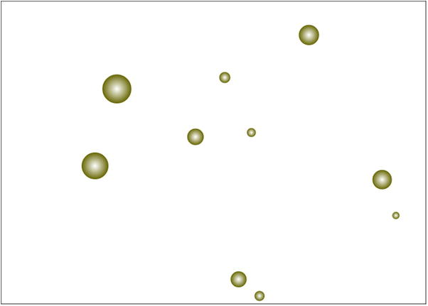
Figure 11-15. “Molecules” bouncing off each other and off walls
You may also find that some particles overlap when they are initially created because of the random positioning. This will result in some initial erratic behavior that should mostly sort itself out in a few timesteps. Other problems could also occur with numerous particles (apart from the obvious one of your computer not being able to cope), especially if they are crammed into a small space or if they are moving at high speed. You could, for example, have a particle colliding with two other particles in the same timestep. Or you could have a particle that is repositioned and ends up overlapping another particle close by. We could go into elaborate methods for dealing with scenarios like these, but we’ve already covered a lot of ground in this chapter and need to stop somewhere!
Summary
In this chapter, we have gone from a simple demonstration of a ball bouncing off a vertical wall to creating complex simulations involving particles bouncing off multiple inclined walls and particles colliding with other particles. We have covered the underlying physics in considerable detail, discussing the equations that govern different types of collisions in 1D and 2D. In implementing collision resolution, both with walls and between particles, we introduced a novel method using vector algebra that avoids the usual need for performing coordinate rotations to resolve collisions in 2D. The range of examples we looked at culminated in an interesting simulation with multiple particles colliding and behaving like the molecules of a gas. In the next chapter we continue the fun by exploring a range of visual and animated effects that can be achieved with systems involving a large number of particles.