**3.7. Arithmetic on Hyperelliptic Curves

Let be a finite field and C a hyperelliptic curve of genus g defined over K by Equation (2.13), that is, by

C : Y² + u(X)Y = v(X)

for suitable polynomials u, . We want to implement the arithmetic in the Jacobian . Recall from Section 2.12 that an element of can be represented uniquely as a reduced divisor Div(a, b) for a pair of polynomials a(x), with a monic, deg_x a ≤ g, deg_x b < deg_x a and a|(b² + bu – v). Thus, each element of requires O(g log q) storage.

3.7.1. Arithmetic in the Jacobian

We first present Algorithm 3.34 that, given two elements Div(a₁, b₁), Div(a₂, b₂) of , computes the reduced divisor Div which satisfies Div(a, b) ~ Div(a₁, b₁) + Div(a₂, b₂). The algorithm proceeds in two steps:

Both these steps can be performed in (deterministic) polynomial time (in the input size, that is, g log q). Algorithm 3.34 implements the first step and continues to work even when the input divisors are semi-reduced (and not completely reduced).

Algorithm 3.34. Sum of semi-reduced divisors

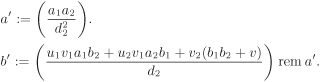
It is an easy check that the two expressions appearing between pairs of big parentheses in Algorithm 3.34 are polynomials. This algorithm does only a few gcd calculations and some elementary arithmetic operations on polynomials of K[X]. If the input polynomials (a₁, a₂, b₁, b₂) correspond to reduced divisors, then their degrees are ≤ g and hence this algorithm runs in polynomial time in the input size. Furthermore, in that case, the output polynomials a′ and b′ are of degrees ≤ 2g.

We now want to compute the unique reduced divisor Div(a, b) equivalent to the semi-reduced divisor Div(a′, b′). This can be performed using Algorithm 3.35. If the degrees of the input polynomials a′ and b′ are O(g) (as is the case with those output by Algorithm 3.34), Algorithm 3.35 takes a time polynomial in g log q. To sum up, two elements of can be added in polynomial time. The correctness of the two algorithms is not difficult to establish, but the proof is long and involved and hence omitted. Interested readers might look at the appendix of Koblitz’s book [154].

For an element and , one can easily write an algorithm (similar to Algorithm 3.9) to compute nα using O(log n) additions and doublings in .

3.7.2. Counting Points in Jacobians of Hyperelliptic Curves

For a hyperelliptic curve C of genus g defined over a field , we are interested in the order of the Jacobian rather than in the cardinality of the curve . Algorithmic and implementational studies of counting have not received enough research endeavour till date and though polynomial-time algorithms are known to this effect (at least for curves of small genus), these algorithms are far from practical for hyperelliptic curves of cryptographic sizes. In this section, we look at some of these algorithms.

Algorithm 3.35. Reduction of a semi-reduced divisor

We start with some theoretical results which are generalizations of those for elliptic curves. The Frobenius endomorphism , x ↦ x^q, is a (non-trivial) -automorphism of . The map naturally (that is, coordinate-wise) extends to the points on and also to divisors and, in particular, to the Jacobian as well as to . For a reduced divisor Div, we have , where for a polynomial the polynomial is obtained by applying the map to the coefficients of h. It is known that satisfies a monic polynomial χ(X) of degree 2g with integer coefficients. For example, for g = 1 (elliptic curves) we have

χ(X) = X² – tX + q,

where t is the trace of Frobenius at q. For g = 2, we have

Equation 3.7

for integers t₁, t₂. The cardinality is related to the polynomial χ(X) as

and satisfies the inequalities

Equation 3.8

Thus n lies in a rather narrow interval, called the Hasse–Weil interval, of width ,

Theorem 2.50 can be generalized as follows:

Theorem 3.6. Structure theorem for

The exponent of (See Exercise 3.42) is clearly m := Exp . Since m|n, there are ≤ ⌈(w + 1)/m⌉ possibilities for n for a given m (where w is the width of the Hasse–Weil interval). In particular, n is uniquely determined by m, if m > w. From the Hasse–Weil bound, we have , that is, . There are examples with . On the other hand, . So it is possible to have m ≤ w, though such curves are relatively rare. In the more frequent case (m > w), Algorithm 3.36 determines n.

Algorithm 3.36. Hyperelliptic curve point counting

Since Exp , the above algorithm eventually (in practice, after few executions of the while loop) computes this exponent. However, if Exp , the algorithm never terminates. Thus, we may forcibly terminate the algorithm by reporting failure, after sufficiently many random elements x are tried (and we continue to have m ≤ w). In order to complete the description of the algorithm, we must specify a strategy to compute ν := ord x for a randomly chosen . Instead of computing ν directly, we compute an (integral) multiple μ of ν, factorize μ and then determine ν. Since nx = 0, we search for a desired multiple μ in the Hasse–Weil interval. This search can be carried out using a baby-step–giant-step (Section 4.4) or a birthday-paradox (Exercise 2.172) method, and the algorithm achieves an expected running-time of which is exponential in the input size. This method, therefore, cannot be used except when n is small.

For hyperelliptic curves of small genus g, generalizations of Schoof’s algorithm (Algorithm 3.31) can be used. Gaudry and Harley [106] describe the case g = 2. One computes the polynomial χ(X) of Equation (3.7), that is, the values of t₁ and t₂ modulo sufficiently many small primes l. Since the roots of χ(X) are of absolute value , we have and |t₂| ≤ 6q. Therefore, determination of t₁ and t₂ modulo O(log q) small primes l uniquely determines χ(X) (as well as n = χ(1)).

Let be the set of l-torsion points of . The Frobenius map restricted to satisfies

Equation 3.9

where t_{1, l} := t₁ rem l, t_{2, l} := t₂ rem l and q_l := q rem l. By exhaustively trying all (that is, ≤ l²) possibilities for t_1,l and t_2,l, one can find out their actual values, that is, those values that cause the left side of Equation (3.9) to vanish (symbolically).

A result by Kampkötter [144] allows us to consider only the reduced divisors of the form D = Div(a, b) with a(X) = X² + a₁X + a₀ and b(X) = b₁X + b₀. There exists an ideal of the polynomial ring such that a reduced divisor D of this special form lies in if and only if f(a₁, a₀, b₁, b₀) = 0 for all . Thus the computation of the left side of Equation (3.9) may be carried out in the ring . An explicit set of generators for can be found in Kampkötter [144]. To sum up, we get a polynomial-time algorithm.

Working (modulo ) in the 4-variate polynomial ring is, indeed, expensive. Use of Cantor’s division polynomials [43] essentially reduces the arithmetic to proceed with a single variable (instead of four). We do not explore further along this line, but only mention that for g = 2 Schoof’s algorithm employing division polynomials runs in time O(log⁹ q). Although this is a theoretical breakthrough, the prohibitively large exponent (9) in the running-time precludes the feasibility of using the algorithm in the range of interest in cryptography.

Exercise Set 3.7