
3 Digital Interperiod Signal Processing Algorithms
3.1 Digital Moving-Target Indication Algorithms
The main fundamental theoretical principles of moving-target indication radar are delivered well in Ref. [1]. The performance of the moving-target indication radar can be greatly improved due primarily to four advantages:
Increased stability of radar subsystems such as transmitters, oscillators, and receivers
Increased dynamic range of receivers and analog-to-digital converters
Faster and more powerful digital signal processing
Better awareness of the limitations, and therefore requisite solutions, of the adapting moving-target indication radar systems to the environment
These four advantages can make it practical to use sophisticated techniques that were considered, and sometimes tried, many years ago but were impractical to implement. Examples of early concepts that were well ahead of the adaptive technology were the velocity-indicating coherent integrator [2] and the coherent memory filter [3,4].
Although such technological developments are able to augment the moving-target indication radar capabilities substantially, there are still no perfect solutions to all problems encountered with using moving-target indication radars, and the design of moving-target indication radar systems is still as much an art as it is a science. Examples of current problems include the fact that when receivers are built with increased dynamic range, limitations arising out of systemic instability will cause increased clutter residue (relative to system noise), leading to false detections. Clutter maps, which are used to prevent false detections from clutter residues, work quite well on fixed radar systems but are difficult to implement on, for example, shipboard radars, because as the ship moves, the aspect angle and range to each clutter patch changes, creating increased residues after the clutter map. A decrease in the resolution of the clutter map to counter the rapidly changing clutter residue will preclude much of the inter-clutter visibility, which is one of the least appreciated secrets of successful moving-target indication radar operation. The moving-target indication radar must work in the environment that contains strong fixed clutter; birds, bats, and insects; weather; automobiles; and ducting. The ducting is also referred to as anomalous propagation; it causes radar return signals from clutter on the surface of the Earth to appear at greatly extended ranges, which in turn exacerbates the problems with birds and automobiles, and can also cause the detection of fixed clutter hundreds of kilometers away.
3.1.1 PRINCIPLES OF CONSTRUCTION AND EFFICIENCY INDICES
When signal processing is carried out under conditions of correlated passive interferences, an initial optimal signal processing of pulse train from N coherent pulses is reduced to v-fold (v ≤ N) interperiod subtraction of complex amplitude envelopes of the pulse train with subsequent accumulation of uncompensated remainders. A procedure of the interperiod subtraction (equalization) of fixed-position correlated interferences (interferences generated by fixed-position correlated sources) allows us to indicate targets moving relative to radar system. As a rule, this procedure is called the moving-target indication.
About 25–30 years ago, the moving-target indication was carried out by analog wireless devices such as delay circuit, analog filters, and so on. Currently, digital moving-target indicators are widely used for the equalization of passive interferences. The digital moving-target indicators consist of memory devices and digital filters [5–8].
The designing of digital moving-target indicators and the evaluation of their efficiency must take into consideration the following peculiarities:
Using the digit capacity Nb ≥ 8 of the target return signal amplitude samples in the digital moving-target indicator, quantization errors can be considered as the white Gaussian noise that is added to the receiver noise; on account of this, a synthesis of the digital moving-target indicator is carried out using an analog prototype, that is, by the digitization of well-known analog algorithms.
Quantization of the target return signal amplitude samples leads to additional losses under the equalization of passive interferences, compared to that observed with the use of analog moving-target indicators.
The digital moving-target indicators can be presented using both two-channel and single-channel forms. The block diagram of the two-channel digital moving-target indicator is shown in Figure. 3.1. After processing by DGD, the in-phase and quadrature components of the DGD output signal come in at the inputs of two similar digital filters realizing the interperiod subtraction operation. Under single subtraction, the output signals of quadrature channels of the filter can be presented in the following form:
{ZoutI[i]=ZoutDGDI[i]−ZoutDGDI[i−1]ZoutQ[i]=ZoutDGDQ[i]−ZoutDGDQ[i−1].(3.1)

FIGURE 3.1 Flowchart of the two-channel digital moving-target indicator: ISF-v-v-fold interperiod subtraction filter; ZoutMIT1=√(ZoutIi)2+(ZoutQi)2;ZoutMTI2=|ZoutIi|+|ZoutQi|;ZoutMTI3=|max(ZoutIi,ZoutQi)|+0.5|min(ZoutIi,ZoutQi).
In a similar manner, we can obtain the formulas for the filter output signals in the case of any ν-fold (ν ≤ N) interperiod subtraction when ν = 2, 3,… There is a need to take into consideration that the operations are realized on the signals obtained within the limits of the same sampling interval under sampling in time and the index i denotes the current value of the sweep. Thus, the signals ZoutI[i]
In practice, the following indices are widely used for the evaluation of the efficacy of digital moving-target indicators:
The coefficient of interference cancellation Gcan that is defined as a ratio of the passive interference power at the equalizer input to the passive interference power at the equalizer output
Gcan=PinpiPoutpi=σ2piinσ2pioutatσ2piin≫σ2n,(3.2)
Gcan=PinpiPoutpi=σ2piinσ2pioutatσ2piin≫σ2n,(3.2) where
Pinpi
Pinpi is the power of the passive intereference at the equalizer inputσ2piin
σ2piin is the variance of the passive interference at the equalizer inputPoutpi
Poutpi is the power of the passive interference at the equalizer outputσ2piout
σ2piout is the variance of the passive interference at the equalizer outputσ2n
σ2n is the receiver noise
Figure of merit for the case of linear interperiod cancellation of the passive interferences can be defined in the following manner:
η=Pouts/PoutpiPins/Pinpi=PinsPoutpi×PoutsPins=Gcan×Gs,(3.3)
η=Pouts/PoutpiPins/Pinpi=PinsPoutpi×PoutsPins=Gcan×Gs,(3.3) where Gs is the coefficient characterizing a signal passing through the passive interferences equalizer. In general, when a nonlinear signal processing is used, the figure of merit η indicates to what extent the interference power at the equalizer input can be increased, without losses in detection performance.
The coefficient of improvement is a characteristic of the response of the digital moving-target indicator on passive interferences with respect to the averaged response on target return signals:
Gim=Pouts/Poutpi[Pins/Pinpi]Vtg,(3.4)
Gim=Pouts/Poutpi[Pins/Pinpi]Vtg,(3.4) where ¯[Pins/Pinpi]Vtg
[Pins/Pinpi]Vtg¯¯¯¯¯¯¯¯¯¯¯¯¯¯¯¯¯¯ is the SNR at the equalizer input while deciding on the average values with respect to all target velocities.
The aforementioned Q-factors can be determined both for passive interferences equalizer systems using the interperiod subtraction and for equalizer systems with subsequent accumulation of residues after the passive interference cancellation.
3.1.2 DIGITAL REJECTOR FILTERS
The main element of the digital moving-target indicator is the digital rejector filter that can guarantee a cancellation of correlated passive interference. In the simplest case, the digital rejector filter is constructed in the form of the filter with the v-fold (v < N) interperiod subtraction that corresponds to the structure of the nonrecursive filter. The recursive filters are also widely used for the cancellation of passive interferences. Consider briefly the problems associated with the analysis and synthesis of rejector filters.
The signal processing algorithm of the digital nonrecursive filter takes the following form:
ZoutIQnr(nT)=ZoutIQnr[n]=v∑i=0hiZinIQnr[n−i],(3.5)
where
hi is the weight coefficient of the filter
ZinIQnr[n−i]
ZinIQnr[n−i] are in-phase and quadrature components of signal at the filter input (the DGD output)
At ν = 2, (3.5) defines a signal processing algorithm for the nonrecursive filter with the double interperiod subtraction. To define the coefficients of this filter we can set up the following equations:
ΔZoutIQnr[n]=ZinIQnr[n]−ZinIQnr[n−1];(3.6)
ΔZoutIQnr[n−1]=ZinIQnr[n−1]−ZinIQnr[n−2];(3.7)
ZoutIQnr[n]=ΔZoutIQnr[n]−ΔZoutIQnr[n−1]=ZinIQnr[n]−2ZinIQnr[n−1]+ZinIQnr[n−2].(3.8)
Consequently, the filter coefficients are equal to h0 = h2 = 1, h1 = −2, hi = 0 at i > 2. The flowchart of the digital filter with the interperiod subtraction at v = 2, in the case of the single quadrature channel, is shown in Figure 3.2. Similarly, we can derive the filter coefficients at v > 2. So, at v = 3 we obtain h0 = 1, h1 = −3, h2 = 3, h3 = −1, hi = 0 at i > 3; and the signal processing algorithm takes the following form:
ZoutIQnr[n]=ZinIQnr[n]−3ZinIQnr[n−1]+3ZinIQnr[n−2]−ZinIQnr[n−3].(3.9)
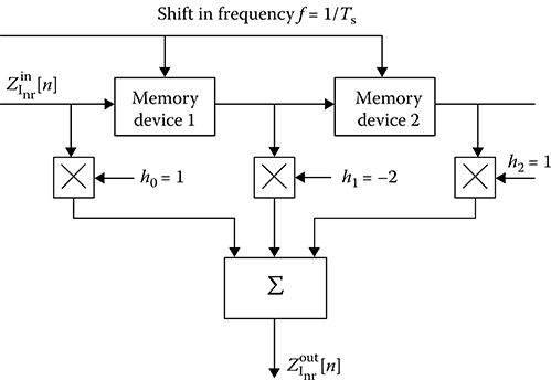
FIGURE 3.2 Flowchart of the digital filter with the interperiod subtraction at v = 2: the in-phase channel.
The digital nonrecursive filters are very simple under realization, but they have very low-angle fronts of the amplitude-frequency performance, which severely affects the effectiveness of passive interference cancellation.
In addition to the nonrecursive filters, the recursive filter can be used as the rejector filter with the following signal processing algorithm:
ZoutIQnr[n]=v∑i=0aiZinIQnr[n−i]+v∑j=0bjZinIQnr[n−j],(3.10)
where ai and bj are the coefficients of the digital recursive filter.
Methods of recursive filter synthesis are considered and discussed in numerous literatures [9-21]. Without going into detail, we note that a synthesis procedure based on a squared amplitude– frequency filter response in accordance with a technique described in Ref. [22] can be considered the most effective for the digital moving-target indicators constructed based on the digital rejector filters. As a first step, and on the basis of the given parameters of environment conditions and initial premises, an order is chosen and the amplitude-frequency characteristic of analog filter prototype is defined. After that we define an approximation of squared amplitude-frequency characteristic of digital filter to the squared amplitude-frequency characteristic of analog filter-prototype, taking into consideration the restrictions arising from structural complexity. The elliptic filter, also known as Zolotaryov-Cauer filter [23], is best suited for these requirements.
Under realization of the digital rejector filter in accordance with (3.10), it is convenient that ai and bj are simple binary numbers. In this case, there is no need to use ROM to store these coefficients, and the multiplication operations are changed by simple shift and summation operations. For example, in the case of the recursive elliptic filter of the second order, synthesized using the squared amplitude-frequency characteristic, we obtain the following values of coefficients [22]: a0 = a2 = 1; a1 = −1.9682; b1 = −0.68; and b2 = −0.4928. To simplify the realization of the digital rejector filter, the coefficients a1, b1, and b2 can be rounded in the following order: a1 = −1.875 = −21 + 2−3, b1 = −0.75 = 20 + 2−3, b2 = −0.5 = −2−1. Investigations showed that rounding off of the coefficients a1, b1, and b2 can give a very small effect on the cancellation of passive interferences; however, this effect is negligible.
The digital rejector filter ensures the best cancellation of passive interferences due to an improvement in the amplitude-frequency characteristic shape, compared with the nonrecursive rejector filter of the same order. However, the degree of correlation of the passive interference remainders at the digital recursive filter output is higher compared to the correlation degree of the passive interference remainders at the digital nonrecursive filter. Moreover, the presence of positive feedback leads to an increase in the duration of transient process and corresponding losses in efficacy if the number of target return pulses in the train is less 20, that is, N < 20.
Now, consider some results of the comparison between the efficiency levels of the digital filter and the analog filter. At first, transform (3.10) to nonrecursive form, that is, present the signal processing algorithm of the digital recursive filter in the following form:
ZoutIQnr[n]=N−1∑i=0hirfZinIQnr[n−i],(3.11)
where
N is the number of pulses in train (sequence)
hirf are the coefficients of digital recursive filter impulse response defined by [23,24]
h0rf=1,hirf=ai+k∑j=1bjhi−jrf.(3.12)
For example, in the case of the digital recursive second-order filter (ν = k = 2) we obtain h0rf = 1, h1rf = a1 + h2rf = a2 + b1h1rf + b2, at i > 2 we have hirf = b1hi−1rf + b2hi−2rf. As follows from (3.12), the impulse response of recursive filter tends to approach infinity and the number of used coefficients is defined by the sample length of the input signal.
Efficiency of interperiod subtraction at different multiplicities of ν can be compared using the coefficient of passive interference cancellation [25]:
Gcan=1∑vi=0∑vj=0bihjρpi[(i−j)T],(3.13)
where
ρpi[·] is the normalized coefficient of interperiod correlation of the passive interferences T is the radar bang period
At determination of Gcan for nonrecursive filters using (3.13) we think that ν is the multiplicity of the interperiod subtraction and for the recursive filters ν = Npi − 1, where Npi is the sample size of passive interferences.
To make calculations using (3.13) there is a need to define a model of interferences. The energy spectrum of passive interferences, that is, the signals reflected from, for example, extended territorial objects, clouds, or other types of reflectors, can be approximated by the Gaussian distribution law given by
fpi(Spi)≈exp[−2.8(SpiΔfpi)2],(3.14)
where
Spi is the energy spectrum of passive interferences
Δfpi is the bandwidth of passive interference spectrum at the level 0.5
The normalized coefficient of correlation corresponding to this spectrum is given as
ρpi(iT)=exp[−π2(ΔfpiiT)22.8].(3.15)
Figure 3.3 represents the coefficient of passive interference cancellation Gcan as a function of Δ fpiiT(i = 1) for various values of multiplicity of interperiod subtractions. As we can see from Figure 3.3, the use of the twofold interperiod subtraction brings a win in cancellation for about 15.dB compared to a single interperiod subtraction. In the case of the threefold interperiod subtraction, a win in cancellation in comparison with the twofold interperiod subtraction is less than 15.dB. In the case of the fourfold interperiod subtraction, a win in cancellation in comparison with the threefold interperiod subtraction is still less. The coefficient of cancellation of passive interferences for recursive filters depends on the sample size Npi of the passive interference. Thus, it is of no use to compare the recursive and nonrecursive filters by the coefficient of passive interference cancellation Gcan. Comparative efficacy of the interperiod subtraction and recursive filters can be evaluated by the figure of merit η given by (3.3), which corresponds to a win in SNR in the case of digital linear filters.
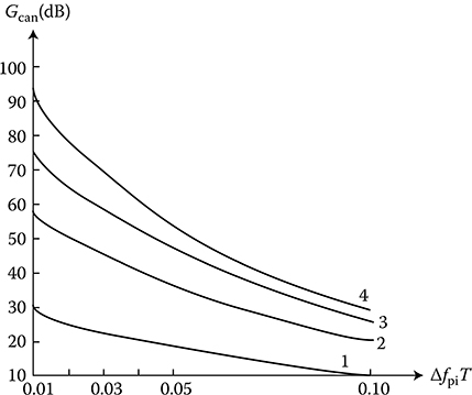
FIGURE 3.3 Coefficient of passive interference cancellation as a function of ΔfpiT(i = 1) for various values of multiplicity of interperiod subtractions: ISF-1, ISF-2, ISF-3, and ISF-4—a single, twofold, threefold, and fourfold interperiod subtraction filters.
Assume that a passive interference source is stationary and fixed, that is, the Doppler shift is zero, ϕD = 0, and the target velocity is optimal, that is, ϕD = π in such a scenario, the figure of merit η can be determined in the following form [24]:
η=∑vsi,j=0(−1)i−jhihjρs[(i−j)T]∑vini,j=1hihjρpi[(i−j)T],(3.16)
where
vs is the sample size of the target return signal equal to Ns − 1 (Ns is the number of target return pulses in train) in the case of recursive filter and the interperiod subtraction multiplicity v in the case of nonrecursive filter
vin is the sample size of interference determined by analogous way as for vs
ρs is the coefficient of correlation of the target return signal
ρpi is the coefficient module of passive interference interperiod correlation
There is a need to define a model of the target return signal for calculations. As a rule, we can think that the target return signal amplitude envelope is subjected to Rayleigh distribution law with the coefficient of correlation defined by
ρs(T)=exp(−πΔftgT),(3.17)
where Δftg is the spectrum bandwidth of the fluctuated target return signal.
The figure of merit η for a set of the digital nonrecursive filters with the twofold (the curve 1) and threefold (the curve 3) interperiod subtractions, the digital recursive filter of the second order (the curve 2), and the digital composite filter consisting of the nonrecursive filter with the single interperiod subtraction and the recursive filter of the second order connected in cascade (the curve 4) is shown in Figure 3.4 as a function of ΔfpiiT (i = 1). As follows from Figure 3.4, the use of digital recursive filters provides a win in 10 dB in the figure of merit in comparison with the use of filters with the interperiod subtraction. The digital recursive filter order and the multiplicity of the interperiod subtraction of the digital nonrecursive filters are the same under comparison.
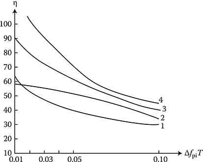
FIGURE 3.4 Figure of merit as a function of ΔfpiT (i = 1) for a set of digital filters: 1—the digital nonrecursive filter with twofold interperiod subtractions; 2—the digital recursive filter of the second order; 3—the digital nonrecursive filter with the threefold interperiod subtractions; 4—the digital composite filter: the digital nonrecursive filter with the single interperiod subtraction plus the digital recursive filter of the second order.
In addition, we can see that the time of transient process in the digital recursive filters is much more in comparison with the time of transient process of the digital nonrecursive filters. Because of this, the interference sample size under the use of the digital recursive filters of the second order must be greater than 20, that is, vin ≥ 20, and vin ≥ 30, if we use the digital recursive filters of the third order. In doing so, the sample size of the target return signal vs does not affect the efficacy of the digital recursive filters of the second and third orders already if vs ≥ 10.
To reduce computer cost under realization of the signal processing algorithm (3.10) using the digital recursive filter, we can implement various computational processes in parallel. As an example, consider a hardware implementation by iteration network [14,26,27]. For this purpose, we can rewrite (3.10) in the following form at v = k = N
Zout[n]=N∑i=0aiDi(Zin[n])−N∑j=1bjDj(Zout[n]),(3.18)
where Di is the operator delaying the input data on i cycles Equation 3.18 can be presented in the following detailed form:
Zout[n]=a0Zin[n]+D1(a1Zin[n]−b1Zout[n])+…+Di(aiZin[n]−biZout[n])+…+DN(aNZin[n]−bNZout[n])
After elementary transformations we obtain
Zout[n]=a0Zin[n]+D1{(a1Zin[n]−b1Zout[n])+D1{(a2Zin[n]−b2Zout[n])+…+D1{(aiZin[n]−biZout[n])+…+D1(aNZin[n]−bNZout[n])}…}.(3.19)
As follows from (3.19), the signal processing algorithm based on the recursive digital filter can be realized using the iteration network (see Figure 3.5) consisting of homogenous elementary blocks with three inputs and a single output and realizing the signal processing algorithm that can be presented in the following form:
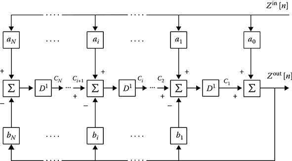
FIGURE 3.5 Digital recursive filter based on the iteration network.
Ci=Ci+1+a1Zin[n]−b1Zout[n],b0=0.(3.20)
Operating speed of the iteration network presented in Figure 3.5 is defined by the operating speed of a single filter cell carrying out two multiplications on constant factors and two summations. Because of this, further increase in the operating speed is made possible using specific structural designs that help with making calculations based on (3.20). When in the considered iteration network all bj = 0 we can obtain a realization of the digital nonrecursive filter. Under the realization of rejector digital filters some specific losses in efficacy occur. The main sources of these losses are quantization of the input signals, rounding-off of the filter weight coefficients, and results of calculations.
As we noted in Section 2.1, under choosing the quantization step Δx based on the condition Δx/σn ≤ 1, where σ2n
σ2out≈σ2n+σ2qn+σ2an.(3.21)
In this case, the resulting value of the figure of merit, taking into consideration the quantization and round-off errors, will be determined as
η′=η1+((σ2qn+σ2an)/σ2n).(3.22)
3.1.3 DIGITAL MOVING-TARGET INDICATOR IN RADAR SYSTEM WITH VARIABLE PULSE REPETITION FREQUENCY
Under indication of moving targets by a complex radar system (CRS) with a constant repetition period of radar searching signal, there take place the so-called “blind” velocities at Doppler frequencies fD = ±k/T, k = 0, 1, 2,… because the phase of the target return signal from moving target varies by 2kπ times within the limits of the period T. To avoid this phenomenon the wobble (modulation) procedure for the repetition period of radar searching signals is used, which leads to the spreading of velocity response of moving-target indication and, finally, to a decrease in the number and depth of dips of resulting velocity response.
Implementation of analog moving-target indicators with the wobble procedure within the limits of the interval T is very difficult, since in this case there is a need to employ various individual delay circuits for each value of repetition period T and complex switching system for these circuits. Under realization of the digital moving-target indicator with the wobble procedure within the limits of the interval T, it is enough to realize only synchronization between a sample of delayed data from memory device and radar searching signal instants. In doing so, the size of memory device does not change and does not depend on the number of discrete values and the wobble procedure function within the limits of the repetition period T. The best speed performance of the digital moving-target indicators with the wobble procedure within the limits of the repetition period T can be obtained if each pulse from the target return pulse train is measured Ns, where Ns is the number of target return pulses in the train adjusted with a new individual repetition period. The individual repetition period T must vary with respect to the average value ˉT
Ti=ˉT+iΔT,i=0,±1,…,±0.5(Ns−1).(3.23)
The problem of design and construction of the digital moving-target indicators with the wobble procedure within the limits of the repetition period T is to make a correct selection of a value ˉT
In the case of coherent pulse radar, we should take into consideration the following conditions choosing the values of ˉT
ˉT−0.5(Ns−1)ΔT≥Tmin.(3.24)
The maximal repetition period Tmax is defined from conditions that are not associated with the digital moving-target indicator operation. Under the given and known values Tmin and Tmax and symmetric disposition of the wobble interval with respect to the value ˉT
ˉT=0.5(Tmin+Tmax).(3.25)
Then, knowing the value of Ns, from (3.25) we can define ΔT.
In general, the wobble procedure is defined by the criterion of figure of merit r) maximization, taking into consideration the minimization of amplitude-frequency characteristic ripple in the digital filter bandwidth. As a rule, this problem is solved by simulation methods. The following wobble procedures are used:
Linear—a consecutive increasing or decreasing T on ±ΔT from pulse to pulse in the train
Cross-sectional analysis, for example, following the procedure
{T2i=ˉT+iΔT,i=0,2,…,0.5(Ns−1)T2i+1=ˉT−(i+1)ΔT,i=1,3,…,0.5(Ns−2)(3.26)
{T2i=T¯¯¯+iΔT,T2i+1=T¯¯¯−(i+1)ΔT,i=0,2,…,0.5(Ns−1)i=1,3,…,0.5(Ns−2)(3.26) Random, for example, by realization of the “bowl” model, restored from the total value of a prior given set T.
Calculations and simulations demonstrate that the wobble procedures for the repetition period T lead to a decrease in the depth of amplitude-frequency response dips of the nonrecursive and recursive digital filters. However, at the same time, a stop band of the nonrecursive and recursive digital filters is narrowed simultaneously with the frequency band extension and distortion of the interference frequency spectrum. By this reason, the effectiveness in cancellation of passive interferences is considerably reduced. Absolute losses in the figure of merit r) for the recursive digital filters of the second order vary from 0.3 to 4.3 dB and from 4 to 19 dB for the recursive digital filters of the third order, in comparison with the digital moving-target indicators without wobble procedures for the repetition period T(at optimal velocity) [28-34].
3.1.4 ADAPTATION IN DIGITAL MOVING-TARGET INDICATORS
In practice, spectral-correlation characteristics of passive interferences are unknown a priori and, moreover, are heterogeneous in space and not stationary in time. Naturally, the efficacy of passive interference cancellation becomes essentially inadequate. To ensure high effectiveness of the digital moving-target indication radar subsystems under conditions of a priori uncertainty and non-stationarity of passive interference parameters, the adaptive digital moving-target indication radar subsystems are employed [4]. In a general sense, the problem of adaptive moving-target indication is solved based on an implementation of the correlation feedback principle [35]. Correlation automatic equalizer of passive interferences represents a closed tracker adapting to noise and interference environment without taking into consideration the Doppler frequency. Parallel with high effectiveness, the tracker has a set of the following imperfections:
Poor cancellation of area-extensive interference leading edge that is a consequence of high time constant value (for about 10 resolution elements) of adaptive feedback
Decrease in passive interference cancellation efficiency over the powerful target return signal
Very difficult realization, especially using digital signal processing
The problem of moving-target indicator adaptation can be solved using the so-called empirical Bayes approach using of which we at first, define the maximal likelihood estimation (MLE) of passive interference parameters and after that we use these parameters to determine the impulse response coefficients of rejector digital filter. In this case, we obtain an open-loop adaptation system, a transient process that is carried out within the limits of transient process of the digital filter.
The first simplest adaptation level in the open-loop adaptation system is to cancel the average Doppler frequency of passive interference caused by relocating to an interference source relative to radar system. In this case, an estimator of the average Doppler frequency of passive interference ¯fDpi
ΔˆˉφDpi=arctan∑ki=1(ZinI1iZinQ2i−ZinI2iZinQ1i)∑ki=1(ZinI1iZinI2i+ZinQ1iZinQ2i),(3.27)
where ZinI1,ZinQ1
˙Zin[n−1]=ZinI[n−1]+jZinQ[n−1](3.28)
on the angle ΔˆˉφDpi
{Z′Iin[n−1]=ZinI[n−1]cosΔˆˉφDpi−ZinQ[n−1]sinΔˆˉφDpi,Z′Qin[n−1]=ZinI[n−1]sinΔˆˉφDpi+ZinQ[n−1]cosΔˆˉφDpi.(3.29)
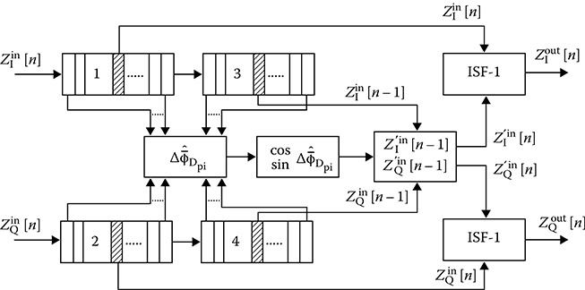
FIGURE 3.6 Block diagram of digital signal processing algorithm used by the digital moving-target indicator under adaptation to target displacement: memory devices 1, 2, 3, and 4.
Flowchart of digital signal processing algorithm used by the digital moving-target indicator under adaptation to the displacement of passive interference source is shown in Figure 3.6. The block diagram consists of memory devices to store the four (k − 1)-fold samples of input signals for each element of radar range along with normal elements; digital signal processing circuits to determine ΔˆˉφDpi,cosΔˆˉφDpi,sinΔˆˉφDpi,Z′Iin[n−1],Z′Qin[n−1]
3.2 DGD for Coherent Impulse Signals with Known Parameters
3.2.1 INITIAL CONDITIONS
In digital signal processing systems, a process of accumulation and signal detection is realized, as a rule, at video frequency, after the union of in-phase and quadrature channels. Henceforth, the signal detection problems will be solved taking into consideration the following initial conditions:
A single input signal can be presented in the following form:
Xi=X(ti)=S(ti,α)+N(ti),(3.30)
Xi=X(ti)=S(ti,α)+N(ti),(3.30) where S(ti, α) is the target return signal (information signal, i.e., the signal containing an information about parameters of the target), α is the function of time and signals parameters, and N(ti)
N(ti) is the noise. The signal parameters are the delay td and direction of arrival θ The total target return signal is a sequence of periodically repeated pulses (the pulse train). At uniform rotation of radar antenna in the searching plane, the pulse train is modulated by directional diagram envelope of the radar antenna. The number of pulses in train is given asNp=φddfVA,(3.31)
Np=φddfVA,(3.31) where
ϕdd is the width of radar antenna directional diagram in the searching plane at the given power P level
f is the pulse repetition frequency of searching signals
VA is the scanning speed of antenna beam
Under discrete scanning in radar systems with phase array the pulse train envelope of the target return signals has a square shape and the number of pulses in train is defined based on the predetermined probability of detection at the searching target zone edge with minimal effective scattering surface. As for the statistical characteristics of the target return signal (information signal), as usual, we consider two cases:
The train of nonfluctuated pulses
The train of independently fluctuating pulses obeying to the Rayleigh pdf with zero mean and the variance σ2s
σ2s , that is,p(Si)=Siσ2Sexp{−S2i2σ2s}.(3.32)
p(Si)=Siσ2Sexp{−S2i2σ2s}.(3.32)
Under synthesis of signal detection algorithms and evaluation of target return signal parameters we use, as a rule, a noise model in the form of Gaussian random process with zero mean and the variance σ2n
σ2n . When the correlated time interferences (namely, passive interferences) are absent, noise samples modeled by the Gaussian process do not have an interperiod correlation. When the passive interferences or their remainders are present after cancellation by the digital moving-target indicators, a sequence of passive interference samples are approximated by Markov chain. To describe statistically the Markov chain we, in addition to the variance, should know the coefficient module ρpi of passive interference interperiod correlation. The interperiod correlation coefficient of the uncorrelated noise with the variance σ2nσ2n and correlated passive interference with the variance σ2piσ2pi can be presented in the following form:ρij=σ2piρpiij+σ2nδijσ2Σ,(3.33)
ρij=σ2piρpiij+σ2nδijσ2Σ,(3.33) where
σ2Σ=σ2pi+σ2n;δij=1 at i=jandδij=0 at i≠j.(3.34)
σ2Σ=σ2pi+σ2n;δij=1 at i=jandδij=0 at i≠j.(3.34) As an example of additional non-Gaussian noise, we can consider a random pulse interference generated by other sources of radiation. This interference is characterized by the off-duty ratio Qpulsein
Qpulsein and amplitude ZpulseinZpulsein that are random variables. Analysis of the stimulus of random pulse interference under signal processing is carried out, as a rule, by simulation methods.Samples of the input signal Xi in the case of absence of target reflecting surface fluctuations are subjected to the general Rayleigh pdf (the hypothesis ℋ1—a “yes” signal)
pℋ1SN(Xi)=Xiσ2Σexp{−X2i+S2i2σ2Σ}I0(XiSiσ2Σ),Xi>0,(3.35)
pH1SN(Xi)=Xiσ2Σexp{−X2i+S2i2σ2Σ}I0(XiSiσ2Σ),Xi>0,(3.35) where I0(x) is the zero-order Bessel function of the first kind. In the case of presence of target reflecting surface fluctuations, we can write
p′ℋ1SN(Xi)=Xiσ2Σ+σ2Siexp{−X2i2(σ2Σ+σ2Si)},(3.36)
p′H1SN(Xi)=Xiσ2Σ+σ2Siexp⎧⎩⎨⎪⎪−X2i2(σ2Σ+σ2Si)⎫⎭⎬⎪⎪,(3.36) where σ2Si
σ2Si is the variance of target return signal amplitude Introduce the following notations: xi = Xi/σ∑ is the relative envelope amplitude; qi = Si/σE is the SNR by voltage; k2i=σ2Si/σ2Σk2i=σ2Si/σ2Σ is the ratio of the target return signal amplitude variance to the interference amplitude variance. Using these notations, we can rewrite (3.35) and (3.36) in the following form:pℋ1SN(xi)=xiexp{−x2i+q2i2}I0(xi,qi),(3.37)
pH1SN(xi)=xiexp{−x2i+q2i2}I0(xi,qi),(3.37) p′ℋ1SN(xi)=xi1+k2iexp{−x2i2(1+k2i)}.(3.38)
p′H1SN(xi)=xi1+k2iexp{−x2i2(1+k2i)}.(3.38) If the target return signal is absent in the input signal, the pdf is the same for the considered cases, that is,
pℋ0N(xi)=xiexp{−0.5x2i}.(3.39)
pH0N(xi)=xiexp{−0.5x2i}.(3.39) The joint pdf of pulse train from uncorrelated normalized samples in the case of absence of target reflecting surface fluctuations (uniform radar antenna scanning) takes the following form:
pℋ1SN(x1,x2,…,xN)=pℋ1SN{x}N=N∏i=1{xiexp{−x2i+q2i2}I0(xi,qi)},(3.40)
pH1SN(x1,x2,…,xN)=pH1SN{x}N=∏i=1N{xiexp{−x2i+q2i2}I0(xi,qi)},(3.40) where
qi = q0gi, gi are the weight coefficients depending on the radar antenna directional diagram shape
q0 is the SNR at the maximum power of radar antenna directional diagram
Similarly, for the pulse train from N samples in the case of Rayleigh fluctuations of the target return signal (the target reflecting surface fluctuations), we can write
pℋ1SN{x}{xi1+k2iexp{−x2i2(1+k2i)}}=N∏i=1{xi1+k2iexp{−x2i2(1+k2i)}}.(3.41)
pH1SN{x}{xi1+k2iexp{−x2i2(1+k2i)}}=∏i=1N{xi1+k2iexp{−x2i2(1+k2i)}}.(3.41) In the case of discrete radar antenna scanning, (3.40) and (3.41) have the same form under the conditions
x1=x2=…=xN,ai=a0,k1=k0,gi=1.(3.42)
x1=x2=…=xN,ai=a0,k1=k0,gi=1.(3.42) Digital signal detection algorithm is considered for two versions:
The target return signal is quantized by amplitude in such manner that a low-order bit value does not exceed the root-mean-square value σn of receiver noise. In this case, a stimulus tracking of quantization by amplitude is added up to an addition of independent quantization noise to the input noise and a synthesis of digital signal processing algorithms is reduced to digital realization of optimal analog signal processing algorithms [36]
The target return signal is quantized on two levels—binary quantization. In this case, there is a need to carry out a direct synthesis of signal processing algorithms and decision-making networks to process digital binary quantized signals. The required probability of signal detection PD and the probability of false alarm PF take the following form [37–40]:
PD{di}=N∏i=1PdiSNib(1−di)SNi;(3.43)
PD{di}=∏i=1NPdiSNib(1−di)SNi;(3.43) PF{di}=N∏i=1PdiNib(1−di)Ni;(3.44)
PF{di}=∏i=1NPdiNib(1−di)Ni;(3.44)
where
PdiSNi
PdiSNi is the probability of detectionPdiNi
PdiNi is the probability of false alarm of the i-th target return signal from the pulse train that can be presented in the following form:PSNi=∞∫c0Pℋ1SN(xi)dxi,bSNi=1−PSNi;(3.45)
PSNi=∫c0∞PH1SN(xi)dxi,bSNi=1−PSNi;(3.45) PNi=∞∫c0Pℋ1N(xi)dxi,bNi=1−PNi;(3.46)
PNi=∫c0∞PH1N(xi)dxi,bNi=1−PNi;(3.46)
and
di={1,ifxi≥c00,ifxi<c0,(3.47)
di={1,0,ififxi≥c0xi<c0,(3.47) where c0 is the normalized threshold for binary signal quantization by amplitude.
3.2.2 DGD FOR TARGET RETURN PULSE TRAIN
DGD is discussed in detail for a variety of applications in Refs. [39,40,42-69]. In this section we present a brief analysis of the digital signal processing algorithms based on the generalized approach to signal processing in noise. Our main goal in this section is to compare the work content of DGD realization with other digital signal processing algorithms. First, consider the case when the parameters of target return signals—the pulse train from N nonfluctuating pulses with the additive receiver noise with known statistical characteristics—are known.
Based on the theoretical analysis carried out in Refs. [41,44,45], we can write the likelihood ratio for the generalized signal processing algorithm in the following form:
ℒg=pℋ1SN{xi}pℋ0N{˜xi}=N∏i=1exp[−0.5q2i]I0[2xiqi−x2i+˜x2i],(3.48)
where ˜xi
N∏i=1exp[−0.5q2i]I0[2xiqi−x2i+˜x2i]≥Kg.(3.49)
Taking logarithm and making some mathematical transformations with respect to (3.49), we can write
N∑i=1lnI0[2xiqi−x2i+˜x2i]≥lnKg+N∑i=10.5q2i.(3.50)
Further mathematical transformations of (3.50) are associated with an approximation of the function ln I0(x). In the case of weak signals, that is, qi ≪ 1, we use the following approximation
lnI0[2xiqi−x2i+˜x2i]≈12xiq2i−x2i+˜x2i.(3.51)
Consequently, taking into consideration that qi = q0gi and gi are the weight coefficients depending on the radar antenna directional diagram shape, the detection algorithm of weak target return pulse train will have the following form:
N∑i=1[2g2ix2i−x4i+˜x4i]≥K′g,whereK′g=lnKgq20+0.5q20N∑i=1g2i.(3.52)
Now, consider the case of powerful signals, that is, qi ≫ 1. In this case, we use the following approximation:
lnI0[2xiqi−x2i+˜x2i]≈2xiqi−x2i+˜x2i.(3.53)
Consequently, taking into consideration that qi = q0gi and gi are the weight coefficients depending on the radar antenna directional diagram shape, the detection algorithm of powerful target return pulse train will have the following form:
N∑i=1[2gixi−x2i+˜x2i]≥K′g,whereK′g=lnKg2q0+0.5q0N∑i=1g2i,(3.54)
Thus, in the case of the target return pulse train with completely known parameters and modulated by the radar antenna directional diagram, the generalized signal detection algorithm comes to weight summation of normalized samples of the target return pulse train and implementation of energy detector at the output of quadrature or linear detector within the limits of target return pulse train bandwidth and comparison of accumulated statistic with the threshold K′g
In practice, when the real radar system is employed, the target return pulse train contains the unknown parameters, such as SNR, that is, q0, at the maximum point of radar antenna directional diagram, the delay td of the target return pulse train relative to searching/scanning signal, and angular defection of the target return pulse train center θ in the scanning plane with respect to the fixed direction θ0. Because of this, to process information completely inside the radar coverage a realization of generalized signal detection algorithm should be organized within the limits of each interval of time sampling or radar range discretization. Accumulation of processed signals must be carried out within the limits of “tracking/moving window.” The length of “tracking/moving window” must be equal to the number of target return pulses in train. In this case, at the low SNR (for rth sampling or discretization interval) the generalized detection algorithm of nonfluctuating target return pulse train (there are no fluctuations of the target reflecting surface) can be presented in the following form:
ln{ℒ(r)gμ}=N−1∑i=0[2g2i(x(r)μ−i)2−(x(r)μ−i)4+(˜x(r)μ−i)4]≥K′g,r=1,2,…,M,M=TTs,μ≥N;(3.55)
The generalized detection algorithm of fluctuating target return pulse train (there are fluctuations of the target reflecting surface) can be presented in the following form (at q0 ≪ 1):
ln{ℒ(r)gμ}=N−1∑i=0[2g2ik2i1+g2ik2i(x(r)μ−i)2−(x(r)μ−i)4+(˜x(r)μ−i)4]≥K′g.(3.56)
In the case of powerful signal, the generalized signal detection algorithm within the limits of the “tracking/moving window” is obtained by analogous way. Thus, the DGD of target return pulse train with unknown parameters represents a composition of the “tracking/moving window” summator and energy detector with the threshold network and signal generator indicating a detection of the target return pulse train.
3.2.3 DGD FOR BINARY QUANTIZED TARGET RETURN PULSE TRAIN
Now, consider the case when the input sequences are quantized on two levels by amplitude. The generalized detection algorithm of binary quantized target return pulse train is obtained from a synthesis of the likelihood ratio comparing it with the threshold. In doing so, we use the probability of signal detection PD and the probability of false alarm PF given by (3.43) and (3.44). The obtained generalized signal detection algorithm has the following form in its final version:
ln{ℒ(r)gμ}=N−1∑j=0χjd(r)μ−j≥K′g,(3.57)
where the weight coefficients and the threshold are given by
χj=lnPSNbNPNbSNj;(3.58)
K′g=lnKg−N−1∑j=0bSNjbN;(3.59)
and
PSNj=∞∫c0xjexp{−x2j+q2j2}I0(xj,qj)d(xj);bSNj=1−PSNj(3.60)
is the probability to get the unit on the jth position of the target return pulse train;
PN=∞∫c0xjexp{−x2j2}d(xj);bN=1−PN(3.61)
is the probability to get the unit in noise region (a “no” signal);
dμ−j={1,ifzinμ−j≥c00,ifzinμ−j<c0,(3.62)
where c0 is the normalized threshold for binary signal quantization by amplitude.
Thus, the generalized signal detection algorithm for the binary quantized target return pulse signals comes to summation of the weight coefficients χj corresponding to positions of the target return pulse train where d(r)μ−j=1. The generalized signal detection algorithm of nonmodulated target return pulse train (in the case of scanning with the fixed antenna) takes the following form:
ln{ℒgμ}=N−1∑j=0dμ−j≥K″g.(3.63)
In other words, the generalized signal detection algorithm is reduced to accumulation of units within the limits of the target return pulse train length (within the limits of length of the “moving/tracking window” with the predetermined sampling increment) and comparison of the obtained end sum with the threshold.
3.2.4 DGD BASED ON METHODS OF SEQUENTIAL ANALYSIS
The use of methods of the sequential analysis takes a very important place in signal detection theory. Detectors constructed based on methods of the sequential analysis allow us to determine the logarithm of likelihood ratio by the following recurrence formula [70-75]
ln{ℒgμ}=ln{ℒgμ−1}+ln{Δℒgμ},(3.64)
where
ℒgμ−1 is the accumulated likelihood ratio over μ − 1 steps
Δℒgμ is the likelihood ratio increment at the μ-th step of sequential analysis
The accumulated step-to-step statistic ln{ℒgμ} is compared with the upper ln A and lower ln B thresholds
lnA=lnPDPFandlnB=ln1−PD1−PF,(3.65)
where
PD is the predetermined probability of detection
PF is the predetermined probability of false alarm, correspondingly
If following a comparison we have
ln{ℒgμ}≥lnA,(3.66)
the decision about signal detection is accepted and we stop analysis. If following a comparison we obtain
ln{ℒgμ}≤lnB.(3.67)
Then the decision about a “no” signal is accepted and we also stop analysis. If the following condition is satisfied
lnB<ln{ℒgμ}<lnA,(3.68)

FIGURE 3.7 Accumulation of statistic and decision-making procedure under the sequential analysis.
we continue an analysis, that is, we observe a new sample and determine the likelihood increment. The process of accumulation of ln{ℒgμ} and making a decision is presented in Figure 3.7.
Logarithm of likelihood increment is determined by the following formula:
ln{Δℒgμ}=lnpSN(xμ)pN(˜xμ).(3.69)
In doing so, in the case of nonfluctuating target return pulse train model (there are no fluctuations of the target reflecting surface), we use the following logarithm of likelihood increment:
ln{Δℒgμ}=lnI0(xμ,qμ)−q2μ2.(3.70)
In the case of rapidly fluctuating target return pulse train model (there are fluctuations of the target reflecting surface), we use the following logarithm of the likelihood increment:
ln{Δℒgμ}=k2μx2μ1−k2μ−ln(1+k2μ),(3.71)
where the parameter k is given by (3.42).
Thus, to realize a procedure of sequential signal detection there is a need to first define the expected SNR by voltage, for example, in the case of nonfluctuating target return pulse train model (there are no fluctuations of the target reflecting surface), and by power in the case of rapidly fluctuating target return pulse train model (there are fluctuations of the target reflecting surface). The main characteristic of sequential analysis procedure is the average number of steps ˉn to make a final decision a “yes” or a “no” signal in the input process. Consider how the average number of steps depends on a “yes” signal and threshold under decision making.
In the case of a “no” signal in the input process, the procedure of sequential analysis is finished by the likelihood ratio logarithm ln{ℒgμ} overrunning the lower threshold ln B. Value of the lower threshold ln B does not depend on the predetermined probability of false alarm PF since the probability of false alarm PF varies within the limits of 10−3 ÷ 10−11 and is only defined by an acceptable value of the probability of miss, that is, PM = 1 − PD, where PD is the probability of signal detection. By this reason, the average cycle of sequential analysis procedure, in the case of a “no” signal in the input process, depends only on the predetermined probability of signal detection PD and increases with increasing in PD.
In the case of a “yes” signal at the DGD input, the procedure of sequential analysis is finished, as a rule, by overrunning the upper threshold ln A. A value of the upper threshold ln A is defined by the predetermined probability false alarm PF. Consequently, the average cycle of analysis in the case of a “yes” signal at the DGD input depends on the predetermined probability of false alarm PF and SNR.
An advantage of the DGD based on the sequential analysis in comparison with the well-known Neyman–Pearson detector consists of the average number of target return signal samples ˉn, which is necessary to make a decision based on the predetermined probability of false alarm PF and probability of signal detection PD is less under sequential analysis procedure than the fixed number of samples N required for the Neyman–Pearson detector. Consequently, it is possible to reduce the computer cost and power energy of a CRS under the detection of target. This possibility can be realized by a radar system with programmable radar antenna scanning when the radar antenna beam can be delayed in scanning direction until the end decision making. However, this advantage has been proved rigorously only in the case of a single channel, that is, under signal detection within the limits of a single radar range resolution interval. In the time of radar signal processing, there is a need to make a decision taking into consideration all elements of radar range resolution simultaneously (multichannel case). In this case, the effectiveness of sequential analysis is defined by the average number of searching radar signals required to make the end decision in all elements of radar range resolution with the predetermined probability of false alarm PF and probability of signal detection PD. This number is determined by the following formula:
ˉn=maxk=¯1,mˉnk,(3.72)
where
m is the number of analyzed resolution elements in radar range
ˉnk is the average cycle of sequential analysis at the kth radar range resolution element
Optimality of sequential procedure in the multichannel radar systems is not proved so far. There are no analytical and theoretical methods and procedures to determine the efficacy of detectors constructed based on the sequential analysis and employed by multichannel radar systems. This is also particularly true for the DGD. For this reason, an analysis of the multichannel radar systems implementing the sequential analysis procedures is carried out using simulation techniques in each particular case. In what follows, we present some results of this analysis.
In the time of sequential analysis in the multichannel radar system there are two possible types of procedures:
Decision making is an independent procedure: In this case, a test for the given channel is finished after reaching one of the thresholds—the upper threshold or the lower threshold.
Simultaneous decision making: This decision making is made if all values of partial likelihood ratios overrun one of the thresholds—the upper threshold or the lower threshold. In this case, multiple crossings of the thresholds are possible.
The average number of tests both for the first case and for the second cases is defined by (3.72). However, the procedure of the second kind is more cost-effective in terms of the required average number of tests since this procedure allows us to level out the lower threshold and, consequently, decrease an uncertainty zone between the upper and lower thresholds. This statement is illustrated in Figure 3.8, where the lower threshold values are demonstrated to make a decision at the predetermined probability of false alarm PF = 10−3 and the probability of signal detection PD = 0.7 for various values of SNR under various ratios of the rapidly fluctuating target return pulse train model (there are fluctuations of the target reflecting surface) to the noise by power as a function of the number m (the number of analyzed resolution elements in radar range). As we can see from Figure 3.8, the value of the lower threshold increases with a corresponding increase in the SNR and m. In this case, at fixed values of the lower threshold, the probability of missing PM of the target return signal decreases inversely to the number m of analyzed resolution elements in radar range; however, in the case of sequential analysis procedure of the first kind, the probability of missing PM of the target return signal is independent of the number m of analyzed resolution elements in radar range.
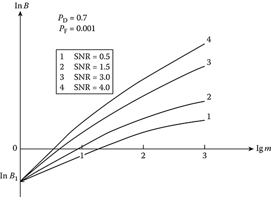
FIGURE 3.8 Simultaneous decision making for multiplicity channel radar systems.

FIGURE 3.9 Average numbers of tests at the sequential analysis versus the number of resolution elements.
In the case of a “no” signal at the DGD input, the average number of tests at sequential analysis procedure in a single receiver antenna radar system depends only on the predetermined probability of signal detection PD. In the multichannel radar system, there is a dependence of the average number of tests at sequential analysis procedure both on the predetermined probability of signal detection PD and on the number m of analyzed resolution elements in the radar range. Dependences between the average number of tests at sequential analysis procedure and the predetermined probability of signal detection PD, the probability of false alarm PF, and (SNR)2 = 1.5 obtained by simulation are presented in Figure 3.9. The average number of tests for a Neyman-Pearson detector are denoted by horizontal lines for each pair of the predetermined probability of signal detection PD and the probability of false alarm PF. The points of intersections of corresponding curves allow us to define the number of analyzed resolution elements in radar range at which the average number of tests for a Neyman-Pearson detector and the average number of tests for the DGD based on sequential analysis procedure is the same. Evidently, the DGD based on sequential analysis procedure is more effective in comparison with the Neyman-Pearson detector if the following condition in the case of a “no” signal
ˉngℋ0seq<ˉnℋ0N−P(3.73)
is satisfied. As follows from Figure 3.9, in the case of a “no” signal at the DGD input the efficacy of the DGD based on sequential analysis procedure is higher, and the predetermined probability of false alarm PF is lower. For a fixed value of the probability of false alarm PF the efficacy of the DGD based on sequential analysis procedure for m receiver antennas increases concomitant to decrease in the probability of signal detection PD.
In the multichannel radar systems, the average number of tests at sequential analysis procedure in the direction of target presence becomes commensurable with the average number of tests at sequential analysis procedure in the direction of target absence even at small numbers of resolution elements. Consequently, the average number of tests at sequential analysis procedure before a decision making is mainly defined by the average number of tests at sequential analysis procedure in the direction of target absence. In the multichannel radar systems, the average number of tests at sequential analysis procedure can be prolonged to such limits that are not acceptable by energy or other tactical considerations. The only way to avoid this prolonged delay of antenna beam in scanning direction is to introduce a truncation procedure of sequential analysis at the ntr-th step and to make a decision about exceeding some fixed threshold C. In this case, the probability of error at the truncation procedure can be presented in the following form:
Ptrer=Per(ˉn<ntr)+Per(C)[1−Per(ˉn<ntr)],(3.74)
where
Per(ˉn<ntr) is the probability of wrong decision at sequential analysis procedure before truncation
Per(C) is the probability of wrong decision at sequential analysis procedure under comparison of decision statistic with the threshold C
Obviously, we can choose such values of ntr and C that additional errors caused by truncation will be satisfied to the following conditions:
PF(C)≤Padd erF−PF(ˉn<ntr),(3.75)
PM(C)≤Padd erM−PM(ˉn<ntr).(3.76)
Algorithm to choose ntr and C satisfying to the conditions (3.75) and (3.76) comes to the following procedure: At n = ntr1 we can choose C such that the first condition given by (3.75) is satisfied. If, at the same time, the second condition given by (3.76) is also satisfied, we stop the procedure of choice. If the (3.76) is not satisfied, we select ntr2 = ntr1 + 1 and test conditions (3.75) and (3.76) again. As was proved by the theory of sequential analysis [25,71], there are the required ntr and C. Introduction of truncation does not effect essentially the average number of tests at sequential analysis procedure in the direction of target absence and slightly reduces the average number of tests at sequential analysis procedure in the direction of target presence.
At binary quantization of the target return pulse train samples, the generalized detection algorithm based on the sequential procedure becomes essentially simple, but the efficacy of detection procedure is decreased. In this case, additional losses in the average number of tests at the sequential analysis procedure can be 15% ÷ 30%. Losses caused by quantization can be reduced to 2%/5% even at 7-8 quantization levels. This fact gives us a reason to design and construct the DGDs based on the sequential analysis procedure with small digit capacity of the target return pulse train samples.
Comparative analysis of effectiveness of the DGD based on the sequential analysis procedure and a detector with the fixed sample volume, for example, the Neyman-Pearson detector, gives rise to a consideration of two-stage signal detection procedure. The two-stage signal detection procedure consists of the following. At first, the target return pulse train sample with the fixed volume n1 is subjected to the generalized signal processing algorithm with the predetermined probability of signal detection PD1 and the probability of false alarm PP1. If the decision a “no” signal is made, the procedure is stopped. Otherwise, an additional procedure is carried out with respect to “suspect data,” and we use for this purpose n2 samples of the target return pulse train and obtain the probability of signal detection PD2 and the probability of false alarm PF2. In doing so, using results of the two stages, we obtain
PD=PD1PD2andPF=PF1PF2.(3.77)
To solve the problem of optimization for the two-stage procedure we can choose such values of n1 and n2 that the average number of tests at sequential analysis procedure would be minimal. In doing so,
{ˉnℋ1=n1+PDˉnℋ12;ˉnℋ0=n1+P′scˉnℋ02,(3.78)
where at PF1 ≪ 1 the probability of duplicate scanning in the a “no” signal direction is defined in the following form:
P′sc=(1−PF1)m1≈m1PF1;(3.79)
where
PF1 is the probability of false alarm at the first stage
ˉnℋ1 is the average number of tests at sequential analysis procedure in the direction of target presence
ˉnℋ0 is the average number of tests at sequential analysis procedure in the direction of target absence
ˉn2ℋ1 is the average number of tests at sequential analysis procedure in the direction of target presence at the second stage
ˉn2ℋ0 is the average number of tests at sequential analysis procedure in the direction of target absence at the second stage
m1 is the number of analyzed resolution elements in radar range at the first stage.
Two-stage DGD based on the sequential analysis procedure allows us to obtain an advantage from 25% to 40% in the average number of tests at sequential analysis procedure in comparison with the DGD or Neyman-Pearson detector with the fixed number of tests subjected to the predetermined probability of signal detection PD and the probability of false alarm PF. Under target detection at high values of the probability of false alarm PF, for example, PF = 103, and at large number of resolution elements, the two-stage DGD can be more effective in comparison with the DGD based on the sequential analysis procedure.
3.2.5 SOFTWARE DGD FOR BINARY QUANTIZED TARGET RETURN PULSE TRAIN
In practice, while designing the detectors for binary quantized target return pulse train, many heuristic methods are used that make a decision about signal detection based on the definition of a unit density within the limits of each sampling interval of the target return pulse train at the envelope detector output. The best-known digital signal processing algorithms from this class of detectors are software algorithms fixing an initial instant of target return pulse train appearance by the presence of l units on m adjacent positions, where l ≤ m, m ≤ 5…10. This is the so-called criterion “ l from m” or “ l/m.” Criterion of the initial instant fixation of target return pulse train appearance is, at the same time, a criterion of target return pulse train detection. To eliminate ambiguity, a criterion of target return pulse train end is defined under an angular coordinate reading. As a rule, the target return pulse train end is fixed by presence of series from k skipping (zeros) one by one (k = 2 … 3). To determine positions between the origin and the end of target return pulse train the binary scalers are employed.
Each of the considered operations can be realized by the digital finite-state automaton. Composition of these digital finite-state automata gives us an example of the software detector block diagram presented in Figure 3.10, where A1 is the digital finite-state machine realizing the detection criterion “ l/m”; A2 is the digital finite-state automaton realizing the criterion of target return pulse train end definition based on series from k zeros; and A3 is the digital finite-state automaton (counter) to determine the number of positions from the instant of target return pulse train detection to the instant of erasing the stored information. Using the well-known methods of abstract digital automata composition [76,77], we are able to obtain the transition matrix and graph of associated automaton realizing a program “l/m - k” for each data pattern l, m, and k. This graph is a starting point to design tools to realize the required digital signal detection algorithm, and the transition matrix allows us to determine rigorously the quality characteristics of software detectors.
Digital storage devices of binary quantized target return pulse train are considered as other groups of detection algorithms for software detectors. The origin of target return pulse train is fixed by the digital storage device by the first unit obtained after counter storage erasing. The target return pulse train end is fixed when a series of k zeros appears, that is, the same principle as for the software detectors. The signal detection is fixed at the instant of counter erasing if the number of storage units is equal or greater than the threshold Nthr. Storage devices of other types are designed in such a way that the counter stores the number of positions (cycles) within the limits of the target return pulse train bandwidth, not the number of units between series from k and more skipping one by one. In doing so, skipping of units at intrinsic positions of target return pulse train is restored. These storage devices are very convenient to realize a digital signal processing algorithm to define the angle coordinate reading of target return pulse train.
Analysis of quality characteristics of the digital software detectors and storage devices can be carried out both by analytic-theoretical method and by simulation. As an example, Figure 3.11 represents the detection performance of software detectors “3/3 - 2,” “ 3/4 - 2,” and “4/5 - 2” and digital storage device of units at the predetermined probability of false alarm PF = 10−4 for the target return pulse train consisting of 15 pulses modulated by the radar antenna directional diagram envelope of the following form:
g(x)=|sinxx|.(3.80)
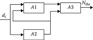
FIGURE 3.10 Software detector block diagram.
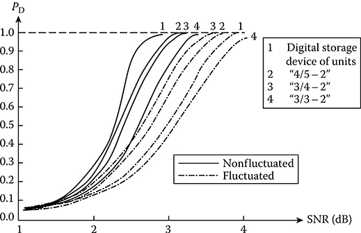
FIGURE 3.11 Detection performance of software detector.
Thresholds of binary quantization are determined by procedures discussed in Ref. [77,78]. The storage device detection threshold (the counter threshold) Nthr is determined in the following form:
Nthr=entier{1.5√N∑i=1gi},i={1,2,…,15}.(3.81)
In the case of absence of target reflecting surface fluctuations under detection of the target return pulse train, the storage devices are more effective in comparison with the software detectors and vice versa; in the case of presence of target reflecting surface fluctuations under detection of the target return pulse train, the software detectors with the detection criterion “l/m” or “l < m” are more effective in comparison with the storage devices.
Threshold losses are low when the target return pulse train is detected by “tracking/moving window” using both the software detectors and the storage devices. Digital realization of these detectors is sufficiently simple, which makes it advantageous to use these detectors when requirements for simplicity of realization prevail over requirements in minimization of energy losses.
It is appropriate to employ the software detectors on the first stage under the two-stage detection procedure.
3.3 DGD For Coherent Impulse Signals with Unknown Parameters
3.3.1 PROBLEM STATEMENTS OF DIGITAL DETECTOR SYNTHESIS
The synthesis problems of optimal detectors are solved with an assumption that there is a priori all information about the noise and interference and their statistical parameters and features under a predetermined energy and statistical characteristics of the target return signal (the information signal). The optimal signal processing and detection algorithms obtained under these conditions possess the best performance for established initial conditions. Changes in noise environment or deviation from characteristics considered under synthesis of detectors leads, as a rule, to a drastic decrease in the efficacy of signal processing and detection algorithms and even to losses in capacity for work.
Detection of target return signals by CRSs in practice is characterized by ambiguity, to a greater or lesser extent, in energy and statistical parameters of signals and noise. In addition, these characteristics are varied in time or are functions of time. In real practice, noise jumping can reach several tens of dB. For example, jumping on 2 ÷ 3 dB only under the fixed detection threshold reduces to changes in the probability of false alarm PF on four orders by magnitude [78]. Thus, a synthesis of robust signal processing and detection algorithms possessing a sufficiently stable quality of service (QoS) under changes in environment conditions is a special interest. As a rule, there is a need to ensure the stability of important QoS only or the probability of false alarm PF only. In this case, we must solve the problem of constant false alarm rate or, in other words, the CFAR problem.
Depending on a priori information about the target return signals and noise, we distinguish the parametric and nonparametric uncertainty. For the parametric uncertainty, the pdf pℋ1XN{xi} under the hypothesis ℋ1 (a “yes” signal) and the pdf pℋ0N{xi} under the hypothesis ℋ0 (a “no” signal) are considered as known pdf, and only some parameters of these pdf are considered as unknown. Changes in environment and external operation conditions are changes in the noise statistical characteristics such as the mean, variance, covariance function, and so on. The robust signal detection algorithms ensuring CFAR are considered, in this case, as adaptive algorithms allowing us to obtain estimations of unknown statistical characteristics of the noise and to employ these estimations to normalize the input signal or to control the threshold. In the second case, the target return signal and noise pdf shape is, as a rule, unknown both at the hypothesis ℋ1 (a “yes” signal) and at the hypothesis ℋ0 (a “no” signal). In this case, a synthesis of robust signal detection algorithms is carried out based on methods of inspection of nonparametric statistical hypotheses. The obtained nonparametric signal detection algorithms bring about the probability of false alarm PF that is independent (or invariant) of the noise envelope pdf pℋ0N{xi}. However, a statistical independence of the target return signal sample values is the indispensable condition of invariance of the nonparametric signal detection algorithms. If there is a correlation between sample values of the target return signal, the mixed signal detection algorithms using parametric and nonparametric statistic are implemented.
The robust signal detection algorithms are able to ensure the best detection performance under the presence of some information about the noise pdf in comparison with the invariant signal detection algorithms and the best stability in comparison with the optimal signal detection algorithms if, in reality, the noise pdf differs from the adopted noise pdf model that is used under synthesis of signal detection algorithms. Ambiguity of the noise statistical characteristics can be given, for example, in the following form for the case of one-dimensional sample:
Pℋ0N{xi}=(1−ε)ˆpℋ0N{xi}+εˆpℋ0N{xi},(3.82)
where
ε > 0 is the infinitesimal real number
ˆpℋ0N{xi} is the known pdf
˜pℋ0N{xi} is the unknown pdf from the given pdf class
When ˆpℋ0N{xi} is the normal Gaussian pdf and the noise samples are uniform, the DGD constructed based on the robust signal detection algorithm must accumulate statistic at the output that is the nonlinear function of Ref. [44], that is,
ZoutDGD(z)={x0,x>x0,x,−x0<x<x0,−x0,x≤−x0.(3.83)
In the case of nonstationary noise (pulse noise, noise “edge”), it is recommended to employ a gate-based signal processing of the target return signal sample in the process of the robust DGD thresh-old computation. One of the simplest examples of such robust signal detection algorithm can be presented in the following form when N is even:
ZoutDGD(x)>Cmax[2N0.5N∑i=1xi,2NN∑i=0.5N+1xi],(3.84)
where
N is the sample size used under threshold computation
C is the constant factor
Efficacy of signal detection algorithms in noise with unknown parameters in comparison with the optimal signal detection algorithms (in the case of known noise parameters) is evaluated by the required increase in the threshold value of SNR to obtain the same QoS. The SNR losses are defined in the following form:
L=10lgq21q20,(3.85)
where
q20 is the threshold SNR ensuring the predetermined probability of detection PD at the some fixed probability of false alarm PF for the optimal signal detection algorithm
q21 is the threshold SNR ensuring the same performance—the probability of detection PD and the probability of false alarm PF for the signal detection algorithm in noise with unknown parameters
To compare the relative efficacy of detectors we can employ the so-called coefficient of asymptotic relative efficiency:
ℱ(A1,A2,PF,PD)=limN1N2→∞N1N2,(3.86)
where N1 and N2 are the sample sizes required for the signal detection algorithms A1 and A2 of two detectors to obtain the same probability of detection PD at the predetermined probability of false alarm PF. In doing so, it is assumed that the total signal energy is independent of the sample size. When ℱ(·) > 1, the signal detection algorithm A1 is more effective in comparison with the signal detection algorithm A2.
3.3.2 ADAPTIVE DGD
To overcome the parametric uncertainty we use estimations of unknown parameters of the target return signal and noise and their pdfs, which are defined by observations [21,27,80-88]. Then these estimations are used under solving the signal detection problems instead of unknown real parameters of the signal and noise. The signal detection algorithms that use the pdfs and their parameters or any other statistical characteristics of signals at the detector input, which are obtained based on estimations, are called the adaptive signal detection algorithms.
When we have information about the presence of an unknown signal parameter θ, the conditional likelihood ratio can be presented in the following form:
ℒ(x|θ)=pℋ1XN{x|θ}pℋ0N{x|θ}.(3.87)
If we are able to define the estimation ˆθ of the signal parameter θ using any statistical procedure, we can determine the likelihood ratio and carry out a synthesis of optimal signal detection algorithm based on the determined likelihood ratio. The estimation of the unknown signal and/or noise parameter is defined by solving the following differential equation:
dp(x|θ)dθ|θ=ˆθ=0.(3.88)
Thus, an essence of adaptation approach is the following. At first, using the limited sample size of input process we define an estimation of the maximal likelihood ratio for unknown parameters of pdf. Then we solve the problem of optimal signal detection at the fixed values of these parameters, that is, θ=ˆθ. Effectiveness of this approach depends on the estimation quality of unknown pdf parameters of signal and noise, which is defined by sample size used to obtain estimations (the training sample).
The main adaptation problem is a stability of false alarm level. For this reason, the adaptive DGD (see Figure 3.12) must have the network calculating an estimation of the current noise parameters (the parameters of the noise pdf). These estimated values of parameters of the noise pdf are used later in the decision statistic generation network, at the output of which we observe the decision statistic given by
ZoutDGD(x)=f{N∑i=1xiσΣi},(3.89)
to normalize the target return signals and noise and, also, to determine the adaptive detection threshold after some functional transformations, where σ2Σi is the total variance.
However, because the sample size used to determine the parameters of the noise pdf and to define the nonstationarity of continuous noise and interference (amplitude jumping of the continuous noise and interference) is limited by m and owing to stimulus of nonstationary noise (e.g., chaotic pulses), there are significant deviations in the probability of false alarm PF from the predetermined value. Moreover, it is characteristic of the fact that these deviations in the probability of false alarm PF are not controlled by the considered adaptive DGD and are not used during an adaptation procedure.
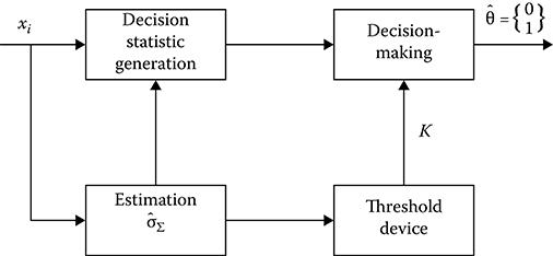
FIGURE 3.12 Adaptive DGD flow chart.
There are specific procedures and methods to reduce an impact of the nonstationarity of continuous noise and interference and chaotic pulse noise and interference in the adaptive DGD. Discuss some of them.
To determine, for example, the total variance σ2Σ=σ2n+σ2in of the noise and interference, assuming that the noise and interference are independent of each other, the noise and interference sampling is carried out under each scanning and in immediate proximity with a resolution element by radar range investigated to give an answer a “yes” or a “no” target. In other words, we employ m time sampling intervals neighboring with the studied resolution element, which are considered as interference. At the same time, we assume that noise samples are uncorrelated and possess a definite stationary by power interval (the quasistationary interval). To reduce an effect of jumping in noise amplitude on the shift of estimation of the variance σ2Σ, for example, to test a “yes” or a “no” target, we select the resolution element (elementary cell) that is in the center of m + 1 adjacent cells or resolution elements. The procedure to estimate the total variance σ2Σ and to normalize the voltage of a “yes” signal elementary cell is explained by Figure 3.13.
To reduce a sensitivity of the total variance σ2Σ to stimulus of powerful interference, for example, chaotic pulse interference, we use a preliminary comparison of the target return signal samples obtained in two adjacent elements of sampling in radar range with follow-up restriction to the threshold used to detect chaotic pulse interference (the method of contrasts) [89]. In accordance with this method, the sampling value xi comes in at the input of total noise variance estimation network if there is no exceeding of the threshold; that is, the condition xi < Cxi − 1 0 < C < 1, is satisfied. If this condition is not satisfied, then a previous result is checked and at xi − 1 < Cxi − 2 the value xi is excluded and the sample size of training sample is decreased on unit. When xi − 1 > Cxi − 2 the sampled value is replaced by the threshold value Cxi −1. The constant factor C is selected in such a way that it will be possible to conform the tolerable losses in the case of interference absence to the required accuracy of estimation of the noise variance in the given range of the off-duty ratio and energy of chaotic pulse interference. Choice of the value C is made, as a rule, based on simulation.
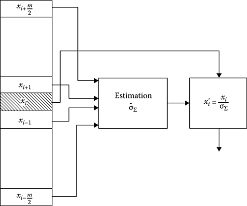
FIGURE 3.13 Procedure of estimation definition of the total variance σ2Σ.
If in the course of training sample analysis there is a possibility not only to detect the chaotic pulse noise but also to measure and define their amplitude, then we can define the value of normalized factor in the adaptive DGD in the following manner. For instance, let l samples of noise from the sample size m are affected by the chaotic pulse noise. Then the estimation of the continuous noise variance (under the normal Gaussian pdf with zero mean) takes the following form:
ˆσ2Σ=m−1∑j=1x2jm−l,(3.90)
and the estimation of the chaotic pulse interference variance is represented in the following form:
ˆσ2chp=1ll∑j=1(Achpj)2,(3.91)
where Achpj is the amplitude of chaotic pulse interference. In the considered case, the target return signal samples must be normalized by the weight
w=11+δ,whereδ=ˆσ2chpˆσ2Σ.(3.92)
This method is effective when the chaotic pulse noise sample is no more than 25%-30% of the training sample and the sample size of the chaotic pulse noise sample is defined by m ≥ 15 … 20.
The considered methods and procedures of adaptation to the noise and interference have a general disadvantage—the number of false signals at the detector output is not registered by any way. Thus, variations in this number of false signals are not detected and the detector is not controlled. In other words, there is no feedback between the detector and the number of false signals. By this reason, the hardware designed and constructed using the principle of closed loop system or open-loop one to control the threshold and decision function and ensuring the CFAR along with normalization is employed in radar systems with the automatic signal processing and signal detection subsystems where CFAR stabilization is very important.
3.3.3 NONPARAMETRIC DGD
Under the nonparametric ambiguity a shape of the pdf p(x) is unknown both in the case of a “yes” signal and in the case of a “no” signal. At this condition, the nonparametric methods of the theory of statistical decisions are employed. This approach allows us to synthesize and design the signal detection algorithms with the predetermined probability of false alarm PF independent of the pdf p(x) shape, that is, with the CFAR in a wide class of unknown pdf p(x) of input signals. Since CFAR is essential for CRS digital signal processing and detection subsystems, there is a great interest to investigate all possible ways to realize the nonparametric signal detection algorithms.
Note that direct values of sample readings of the target return signal are not used by the nonparametric digital detectors. Reciprocal order of the direct values of sample readings of the target return signal is used by the nonparametric digital detectors. This reciprocal order is characterized by the vectors of “sign” and “rank.” By this reason, an initial operation of digital detectors synthesized in accordance with the nonparametric signal detection algorithms is a transformation of the input signal sequence {x1, x2,…, xN} into the sequences of signs {sgn x1, sgn x2,…, sgn xN} or ranks {rank x1, rank x2,…, rank xN}. In doing so, a statistical independence of the input signal sampling readings is the requirement for nonparametric transformation in the classical signal detection problem, that is,
p(x1,x2,…,xN)=N∏i=1p(xi).(3.93)
Principles of designing and constructions of the sign and rank nonparametric detectors are discussed in the following.
3.3.3.1 Sign-Nonparametric DGD
When the input signal or the target return signal is the bipolar pulse, the sample of signs {sgn x1, sgn x2, …, sgn xN} is formed in the following rule:
sgnxi=xi|xi|.(3.94)
Elements of this sample have only two possible values: +1 if xi ≥ 0 and −1 if xi < 0. For the stationary additive noise with the symmetrical pdf with respect to zero, the number of positive and negative signs in the independent noise sample will be the same as N → ∞ When the positive signal appears the probability of the presence of positive signs in the input signal sample becomes higher in comparison with the probability of presence of the negative signs. This phenomenon allows us to detect the target return signal.
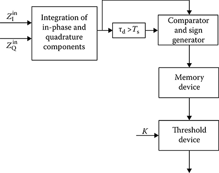
FIGURE 3.14 Flowchart of the sign-nonparametric DGD.
The flowchart presented in Figure 3.14 is employed to obtain the sign sample at the envelope detector output where an integration of in-phase and quadrature components is carried out. The input signals come in at the sign former input by two channels with the delay Ts (the sampling interval of the input signal) at one of them. Delayed and not delayed signals are compared using a comparator. The signals at the comparator output
Δx[kTs]=x[kTs]−x[(k−1)Ts](3.95)
are transformed into signs by the following law:
sgn{Δx[kTs]}={1,ifΔx[kTs]≥0,−1,ifΔx[kTs]<0.(3.96)
For each kth sampling interval (the range ring) by a set of sign sampling
sgn(ik)=sgn{Δx[kTs]},i=1,2,…,N,(3.97)
the signal detection algorithm is realized by the N adjacent scanning periods based on the linear sign statistic
N∑i=1sgn(ik)≥K,(3.98)
where K is the detection threshold defined by the predetermined and acceptable probability of false alarm PF.
The discussed signal detection algorithm implements the method of one-sided contrast [89]. The high value of the contrast function between samples of the target return signal mixed with noise and the noise only is the main precondition under employment of the sign nonparametric generalized signal detection algorithm. There are many modified sign nonparametric signal detection algorithms [70]. QoS of the sign nonparametric signal detection algorithms is characterized by coefficients of asymptotic and relative effectiveness. It is well known that in the case of non-fluctuating target return signal, the coefficient of asymptotic and relative effectiveness of the sign nonparametric generalized signal detection algorithm with respect to the optimal generalized signal detection algorithm is equal to 2/π = 0.65 under the normal Gaussian pdf of the noise; that is, we see that the use of the sign nonparametric generalized signal detection algorithm has a loss rate of 35% in comparison with the optimal generalized signal detection algorithm. Moreover, when the noise is subjected to non-Gaussian pdf, the effectiveness of the sign nonparametric generalized signal detection algorithm can be higher in comparison with the optimal generalized signal detection algorithm.
3.3.3.2 Rank-Nonparametric DGD
To ensure the CFAR under the arbitrary noise pdf, the rank nonparametric detectors are employed. The rank-nonparametric detectors use rank information contained in the sampled sequence of input signals to make a decision. At the same time, the condition of independence of elements of the ranked sample is the indispensable condition also for the sign nonparametric detectors. In practice, under detection of radar signals, when the number of resolution elements (the number of channels) in radar range, in which a “no” signal exists, is much more than the number of resolution signal elements in radar range, in which a “yes” signal exists, we employ the contrast method [89], an essence of which is the following. Each ranked reading si, (i = 1,2,…, N), which is considered as the sample reading of the target return signal, is compared with a set of reference (noise) sample readings wi1, wi2, …, wim taken from the adjacent resolution elements in the radar range. As a result, we determine the reading rank si in the following form:
ri=rank si=m∑i=1Xij,(3.99)
where
Xij={1,ifsi−wij>0,0,ifsi−wij≤0.(3.100)
The ranked and reference samples as well as the results of rank determination can be presented in the following form:
‖s1w11w12………w1ms2w21w22………w2m………………………sNwN1wN2……wNm‖⇒‖r1r2⋮rN‖=RN,ri=1,2,…,m.(3.101)
Further signal processing is to store the rank statistic and compare with the threshold:
N∑i=1ZoutDGD(ri)≥Kg,i=1,2,…,N,(3.102)
where
ZoutDGD(ri) is the known rank function
Kg is the threshold defined based on the acceptable value of the probability of false alarm PF
The simplest rank statistic is the Wilcoxon statistic defined by summation of ranks. By Wilcoxon criterion, the decision a “yes” signal is made in accordance with the following signal detection algorithm:
N∑i=1ri≥Kg,i=1,2,…,N.(3.103)
Relative effectiveness of the rank DGD is higher in comparison with the sign DGD. In the case of the nonfluctuating target return signal and normal Gaussian noise pdf, the relative effectiveness is estimated by 3/π ≈ 0.995. Thus, the rank-generalized signal detection algorithms are practically effective like the optimal generalized signal detection algorithm. A higher level of efficacy of the rank-generalized signal detection algorithms in comparison with the sign generalized signal detection algorithms is obtained owing to the complexity of signal detection algorithm, since ranking of single sample element requires m + 1 summations (subtractions) instead of a single summation (subtraction) per one sample element in the sign signal detection algorithm. Under sequential (moving) rank computation for all resolution elements in radar range, m + 1 summations (subtractions) must be made within the limits of the sampling interval Ts.
In conclusion, there is a need to note that the rank DGD ensures CFAR when the reference sample is uniform, that is, if the noise is a stationary process within the limits of reference sample interval. Reference sample in homogeneity destabilizes the probability of false alarm PF. To reduce this effect there is a need to take appropriate measures, one of which is a rational choice of reference sample arrangement relative to the ranked reading.
3.3.4 ADAPTIVE-NONPARAMETRIC DGD
The nonparametric DGDs do not ensure the CFAR when the correlated noise comes in at the DGD input. For example, in the case of sign-nonparametric DGDs, an increase in the correlation coefficient of input signals from 0 to 0.5 leads to an increase in the probability of false alarm PF on 3 ÷ 4 orders. Analogous and even greater the probability of false alarm PF instabilities takes place in the nonparametric DGDs of other types.
One way to stabilize the probability of false alarm PF at the nonparametric DGD output under the correlated noise conditions is an adaptive threshold tuning subjected to correlation features of the noise [45]. The detector designed and constructed in such a way is called the adaptive-nonparametric DGD. Initial nonparametric signal detection algorithm forming a basis of the adaptive-nonparametric signal detection algorithm must ensure the CFAR when the variance or the noise pdf is varied. The threshold tuning must set off the effect of nonstability of the probability of false alarm PF when the noise correlation function is varied.
The block diagram of the adaptive-nonparametric DGD is shown in Figure 3.15. The nonparametric statistic computer implements a basic function of the initial nonparametric signal detection algorithm:
ZoutDGD(xi)=N∑i=1ςi.(3.104)
If, for example, the initial nonparametric signal detection algorithm is the sign nonparametric signal detection algorithm, then
ςi=sgnxi={1,ifxi≥0,−1,ifxi<0.(3.105)
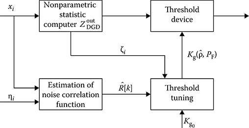
FIGURE 3.15 Flowchart of the adaptive-nonparametric DGD.
To estimate the correlation function of the noise Rn[k] we can use the unclassified sample from the main analyzed sequence {xi}, where i = 1, 2,…, N, and the training reference sample {ηi}. In the case of the use of unclassified sample, the estimate of noise correlation function is determined in the following form:
ˆR[k]=1N−kN−k∑i=1xixi+k−(1NN∑i=1xi),k=0,1,…,N−1.(3.106)
When we know a shape of the noise correlation function Rn[k], for example, the exponential function, that is, Rn[k] = (Rn[1])k or Gaussian, Rn[k] = (Rn[1])k2, then in the case of automatic threshold tuning it is sufficiently to estimate the coefficient of noise interperiod correlation
ˆρ=ˆR[1]ˆR[0],(3.107)
since all other ˆR[k] are related unambiguously with this coefficient. Assuming that the detection threshold Kg depends on the predetermined probability of false alarm PF and the coefficient of noise interperiod correlation, the adaptive-nonparametric generalized signal detection algorithm takes the following form:
ZoutDGD(xi)=N∑i=1ςi≥Kg(ˆρ,PF).(3.108)
Determination of the threshold becomes simple if a sequence of values çi defined by the sequence of values {xi} satisfies the conditions of the central limit theorem for dependent sample readings [90]. Then the pdf of statistic ZoutDGD(xi) forming at the adaptive-nonparametric DGD output is subjected to the asymptotic normal Gaussian pdf. In this case, the probability of false alarm PF can be defined using the following expressions
PF=2Φ{EZ[ˆρ]−Kg(ˆρ,PF)σZ(ˆρ)},(3.109)
where
Φ(x)=1√2πx∫−∞exp(−0.5t2)dt(3.110)
is the standard normal Gaussian pdf defined as [41]
Φ(x)=1−Q(x),(3.111)
where Q(x) is the well-known Q-function given by
Q(x)=1√2π∞∫xexp(−0.5t2)dt.(3.112)
Reference to (3.109) through (3.112) allows us to obtain the algorithm to control and adjust the threshold in the following form:
Kg(ˆρ,PF)=EZ[ˆρ]−Φ−1[0.5PFσZ(ˆρ)],(3.113)
where
EZ[ˆρ] is the mean of decision statistic when the input process samples correlate with each other and this mean is equal to the mean of the decision statistic of the initial nonparametric generalized signal detection algorithm
σ2Z(ˆρ) is the variance of decision statistic when the input process samples correlate with each other
The main problem under synthesis of the adaptive-nonparametric generalized signal detection algorithms is to define the variance of decision statistic at the adaptive-nonparametric DGD output, which depends on input process stationary and the way forming the sequence of values çi.
The adaptive-nonparametric generalized signal detection algorithms with the adaptive tuning threshold based on the sign and rank criteria possess a satisfactory stability to changes in the noise correlation function at the adaptive-nonparametric DGD input. Simulation results show us that with increase in the coefficient of noise interperiod correlation from 0 to 0.5 the probability of false alarm PF at the adaptive-nonparametric DGD output increases by 2 ÷ 5 times, but in the case of the initial sign nonparametric DGD the probability of false alarm PF increases by 100 ÷ 300 times. The adaptive-nonparametric generalized rank signal detection algorithms have analogous characteristics on the stability of the probability of false alarm PF.
In conclusion, we would like to note that the digital adaptive asymptotic optimal generalized signal detection algorithms and the generalized signal detection algorithms using the similarity and invariance principles can be employed in addition to the adaptive-nonparametric generalized signal detection algorithms for signals with the correlated and uncorrelated noise with arbitrary pdf. Each signal detection algorithm has its own peculiarities defining a practicability to use these signal detection algorithms under specific conditions. It is impossible to design the signal detection algorithms that will have the same efficacy when the input signals are not controlled.
3.4 Digital Measurers of Target Return Signal Parameters
Estimation of target return signal parameters comprising information about the coordinates and target characteristics is the main operation of radar signal preprocessing. Estimation of parameters starts after making the decision a “yes” signal; that is, the target has been detected in the direction of radar antenna scanning at the definite distance. At this time, the target detection is associated with rough calculation of target coordinates, for example, the azimuth accurate with the radar antenna directional diagram width and the target range accurate with dimension of the resolution element in radar range and so on. The main task of digital measurer is to obtain more specific information about primary data of estimated target return signal parameters to the predetermined values of target return signal parameters.
Henceforth, we assume that the totality of target return signals, which are used to solve the problem of definition of the target return signal parameters, is within the limits of “moving/tracking window” and dimensions of this “moving/tracking window” correspond to strob bandwidth by radar range and the width of radar antenna directional diagram by angular coordinates. All initial conditions about statistic of the target return signals used under the operation of digital signal processing algorithms of radar signals are kept. We consider uniform estimations of the main no-energy parameters of radar signals, namely, the estimations of angular coordinates, Doppler frequency shift (the radial velocity), and time delay. Quality indices of one-dimensional measurements are the variance of errors σ2θ, where θ = {β, ε, fD, td}, and the work content of the corresponding digital signal processing and detection algorithms.
3.4.1 DIGITAL MEASURER OF TARGET RANGE
Definition of target range by CRSs is carried out as a result of measurements of the time delay td of the target return signal relative to the searching signal in accordance with the formula
td=2rtgc,(3.114)
where c is the velocity of light propagation. In surveillance radar systems with uniform circular (sector) scanning by radar antenna or phased-array radar antenna implemented to define the coordinates a lot of targets, the target range is estimated by readings of the scaled pulses from the instant to send the searching radar signal Δtd1 (the transmit antenna) to the instant to receive the target return signal Δtd2 (the receive antenna, see Figure 3.16). In doing so, with sufficient accuracy in practice, we can believe that there is no target displacement within the limits of receiving the target return pulse train. Consequently, the target range measured by all N pulses of the target return pulse train can be averaged in the following form:
ˆrtg=N∑j=1rtgj,(3.115)
where rtgj is the target range measure by a single reading. The variance of estimation is given by
σ2ˆr=1NN∑j=1σ2rj,(3.116)
where σ2rj is the variance of estimation of the target range measure by a single reading.
Error of a single reading of the time delay td produced by the digital measurer of target range can be presented as a sum of two terms under condition that positions of count pulses on time axis are random variables with respect to the searching signal:
Δtd=Δtd1+Δtd2,(3.117)
where
Δtd1 is the random shift of the first count pulse with respect to the scanning signal
Δtd2 is the random shift of the target return signal with respect to the last count pulse, see Figure 3.16
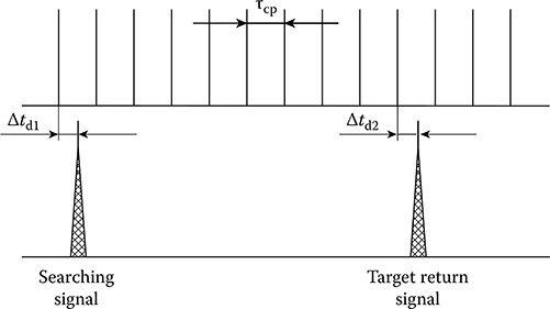
FIGURE 3.16 Definition of the range to target—a time diagram.
These errors are independent random variables uniformly distributed within the limits of the count pulse duration τcp, that is, within the limits of the interval [−0.5τcp, +0.5τcp]. By this reason in this case, the variance of error of a single reading of the time delay td is determined in the following form:
σ2td=16τ2cp.(3.118)
If the initial instant of count pulses is synchronized with the searching signal, in this case, Δtd1 = 0, the variance of error of a single reading of the time delay td is determined in the following form:
σ2td=112τ2cp.(3.119)
The discussed flowchart of digital measurer of the target range can be realized by a specific microprocessor.
3.4.2 ALGORITHMS OF ANGULAR COORDINATE ESTIMATION UNDER UNIFORM RADAR ANTENNA SCANNING
Optimal algorithms to measure the angular coordinate are synthesized by the maximal likelihood ratio criterion, as a rule. The shape of the likelihood function depends on the statistical characteristics of the signal and noise, radar antenna directional diagram shape, and radar antenna scanning technique in the course of measuring. First, we consider the target return pulse train processing that is obtained as a result of uniform rotation of the radar antenna within the limits of radar range sampling interval.
Under multiple-level quantization of the target return signals and weight functions we obtain digital counterpart of optimal measurer of angular coordinate in the scanning plane, that is, for the two-coordinate surveillance radar system—the coordinates of target azimuth βtg. The likelihood function for azimuth estimation by N normalized nonfluctuating target return pulse train in the stationary noise take the following form:
ℒ(x1,x2,…,xN|q0,βtg)=N∏i=1p(xi|qi,βi),(3.120)
where for the considered case we have
p(xi|qi,βi)=xiexp[−0.5(x2i+q2i)]I0(qi,xi).(3.121)
In turn,
qi=q0g(βi,βtg),(3.122)
where q0 is the SNR by voltage in the center of target return pulse train (see Figure 3.17a);
g(βi,βtg)=g[βi−βtgφ0]=g(α)(3.123)
is the function defining the radar antenna directional diagram envelope, for receiving and transmitting in the scanning plane; ϕ0 is the one-half main beam width of the radar antenna directional diagram at zero level; and βi is the value of azimuth angle when receiving the ith pulse of the pulse train.

FIGURE 3.17 (a) Target return pulse train and (b) discrete weight function.
Under the fixed value of q0, we can obtain the final expression of the likelihood function equation for estimation of the angular coordinate βtg in the following form [30,90,91]:
N∑i=1xiγ(βi,ˆβtg)=0,(3.124)
where
γ(βi,ˆβtg)=∂g(βi,ˆβtg)∂ˆβtg,i=1,…,N(3.125)
is the discrete weight function, that is, a sequence of the weight coefficients, to weigh the normalized amplitudes of target return pulse train (see Figure 3.17b). This weight function has a form of discriminatory characteristic, the gain slope of which is a function of the radar antenna directional diagram shape and the zero point coincides with the maximum of the radar antenna directional diagram.
Under estimation of target azimuth angle by the quick-fluctuating target return pulse train, the likelihood function equation takes the following form:
N∑i=1x2iγ′(βi,ˆβtg)=0,(3.126)
where
γ′(βi,ˆβtg)=g(βi,ˆβtg)[1+k20g2(βi,ˆβtg)]2×∂g(βi,ˆβtg)∂ˆβtg,i=1,…,N(3.127)
is the discrete weight function to weight the normalized amplitudes of the target return pulse train from the quick-fluctuating target surface.
Comparing (3.124) and (3.126), we see that in contrast to the case of nonfluctuating target surface to estimate the azimuth angle of target with the quick-fluctuating target surface, there is a need to sum the squared amplitudes of the target return pulse train with their weights. In this case, the weight function γ′(βi,ˆβtg) has a more complex form, but its character and behavior do not change. Thus, the optimal algorithm for the estimation of azimuth target angle under the uniform radar antenna scanning includes the following operations:
The target return pulse train storage in the “moving/tracking window,” the bandwidth of which corresponds to the train time
Weighting of each target return signal amplitude in accordance with the values of corresponding weight coefficients
Formation of half-sum of the weighted target return signal amplitudes observed by the “moving/tracking window” at the right and left sides with respect to zero value of the weight function
Comparison of half-sums and fixation of position where the result of comparison passes through zero value
The simplest example of block diagram of realization of the target azimuth angle coordinate estimation algorithms given by (3.124) and (3.126) is presented in Figure 3.18. In accordance with this block diagram, to realize the target azimuth angle coordinate estimation algorithm there is a need to carry out N − 1 multiplications and N − 1 summations of multidigit binary data while receiving each target return pulse train. The problem of potential accuracy definition of the target azimuth angle coordinate estimation by the target return pulse train can be solved by analytical procedures or simulation with definite assumptions.
Under binary quantization of the target return signal amplitudes (the weight multidigit function), the likelihood function of the estimated target angular coordinate βtg takes the following form:
ℒ(βtg)=N∏i=1PdiSNi(xi)˜P1−diSNi,(3.128)
where
PSNi is the probability that the input signal (the target return signal) exceeds the threshold of binary quantization at the ith position of the target return pulse train
˜PSNi=1−PSNi is the probability to get the unit on the jth position of the target return pulse train di is given by (3.47)

FIGURE 3.18 Block diagram of the target azimuth angle coordinate estimation algorithm given by (3.124) and (3.126).
In the case of nonfluctuating target return signals we can write
PSNi=∞∫c0xiexp{−x2i+q2i2}I0(qi,xi)dxi,(3.129)
and in the case of fluctuating target return signals we have
PSNi=∞∫c0xi1+k2iexp{−x2i2(1+k2i)}dxi.(3.130)
After appropriate mathematical transformations we can write the following likelihood function equation for the considered case
N∑i=1diγ″(βi,ˆβtg)=0,(3.131)
where
γ″(βi,ˆβtg)=1PSNi˜PSNi×dPSNidˆβtg(3.132)
is the weight function of target return pulse train positions under estimation of the target azimuth angle. A type of this function is analogous to the function given by (3.125) in the case of the nonfuctuated target return signal and by (3.127) in the case of the fluctuated target return signal.
Thus, the optimal estimation of target angular coordinate comes to a sum formation of the weight coefficient values y″(βi,ˆβtg) on positions where di = 1 at the right and left sides with respect to zero value of the weight function. Coordinate estimation is fixed when the sums accumulated in this manner are the same within the limits of accuracy given before. Realization of this algorithm of the target return angular coordinate estimation is much simple in comparison with the algorithm given by (3.124) through (3.127), since the multiplication operations of multidigit numbers are absent. Potential accuracy of the measurer designed and constructed based on this algorithm obtained using the Cramer-Rao equality is determined by the formula
σ2ˆβtg1∑Ni=1(dPSNidˆβtg)2×1PSNi˜PSNi.(3.133)
Under binary quantization of the target return signal without taking the radar antenna directional diagram shape into consideration we arrive to heuristic algorithms of the target return angular coordinate estimation:
By a position of the first and last pulses of the target return pulse train
ˆβtg={0.5[λ−(l−1)+μ−k]}Δβ,(3.134)
where
γ is the position number with respect to direction selected as the origin and the first pulse of the target return pulse train is fixed on this position by the criterion of l from m (l/m)
μ is the position number and the last pulse of the target return pulse train is fixed on this position by the criterion of k one after another omission
Δβ is the angular resolution of pulses in train
This algorithm provides for shift compensation of the instant of target return pulse train detection at the (l - 1)th position and a shift of detection instant of the last pulse of train on k positions 2. By a position of the last pulse of the target return pulse train and the number of positions from the first pulse to the last pulse of the target return pulse train
ˆβtg=[μ−0.5(Np−k−1)]Δβ,(3.135)
where Np is the number of positions appropriate to the bandwidth of the detected target return pulse train; this algorithm is realized by digital storage of binary-quantized signals.
Heuristic generalized algorithms of the target return angular coordinate estimation are the simplest in realization but lead us to 25%–30% losses in accuracy in comparison with the optimal generalized signal detection algorithms. Functional dependence of the relative variance of target return angular coordinate estimation, which is given by (3.134) and (3.135), on SNR at the center of target return pulse train at Np = 15 and PF = 10−4 (see Figure 3.19) allows us to compare by accuracy the discussed target return angular coordinate estimation under the uniform radar antenna scanning.

FIGURE 3.19 Relative variance of target return angular coordinate estimation as a function of SNR in the center of the target return pulse train.
3.4.3 ALGORITHMS OF ANGULAR COORDINATE ESTIMATION UNDER DISCRETE RADAR ANTENNA SCANNING
In target tracking and controlling radar systems the methods of monopulse direction finding employed by the multichannel radar systems or the discrete radar antenna scanning employed by the single channel radar systems are used for accurate angular coordinate measurement. In such cases, tracking or nontracking digital measurer can be used. Henceforth, we consider an algorithmic synthesis of the nontracking measurer of a single angular coordinate in the single channel radar system with discrete radar antenna scanning. Under measuring by the discrete scanning method the radar antenna takes two fixed positions (see Figure 3.20). In each fixed position, a direction of maximal radiation with respect to an initial direction corresponds to the angles θ1 and θ2(θ2 > θ1). The difference between angles θ1 and θ2, that is, Δθ = θ2 − θ1 is called the angle of discrete scanning. Under angle readings relative to radar boresight a deviation of maximal radiation at scanning is ±θ0 and a deviation of the target at scanning is θtg.
Measurement of angular coordinate in the discrete radar antenna scanning plane lies in receiving n1 target return signals from direction θ1 and n2 target return signals from direction θ2. Under target displacement θtg with respect to the radar boresight, the amplitudes of target return signals received from each direction are not the same and are equal to X1i and X2i, respectively. We are able to define the azimuth target angle by the amplitude ratio of these target return signals. As before, an optimal solution of the problem of target angular coordinate estimation is defined by maximal likelihood function criterion. In this case, the likelihood function equation takes the following form:
∂ℒ(x1,x2|θtg)∂θtg|θtg=ˆθtg=0,(3.136)
where
x1=‖X11σm1X12σm1…X1m1σm1‖=‖x11x12…x1m1‖T(3.137)
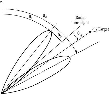
FIGURE 3.20 Fixed positions of radar antenna under discrete scanning.
and
x2=‖X21σn2X22σn2…X2mσn2‖=‖x21x22…x2n2‖T(3.138)
are the vectors of normalized amplitudes of target return signals received from the directions θ1 and θ2, respectively.
The likelihood function of sample ℒ(·) is differed subjecting to accepted models of the signal and noise. When the target return signal fluctuations are absent and the samples are statistically independent, the likelihood function can be presented in the following form:
ℒ(x1x2|θtg)=n1∏i=1pℋ1SN(x1i)n2∏j=1pℋ1SN(x2j),(3.139)
where
pℋ1SN(x1i)=x1iexp{1x21i+q21(θtg)2}×I0[x1i,a1(θtg)],(3.140)
pℋ1SN(x2i)=x2iexp{−x22i+q22(θtg)2}×I0[x2i,a2(θtg)],(3.141)
q1(θtg)=q0g(θtg−θ0)=q0g(θtg+θ0),(3.142)
q2(θtg)=q0g(θ0−θtg),(3.143)
where
g(·) is the normalized function of the radar antenna directional diagram envelope
q0 is the SNR by voltage at the radar antenna directional diagram maximum (the same for both directions)
Substituting (3.139) in (3.136) and taking into consideration (3.140) through (3.143), in the case of powerful target return signal, we get the following result:
lnI0[x1i,a1(θtg)]≈x1iq1(θtg).(3.144)
After evident mathematical transformations we obtain the final likelihood function equation in the following form:
n1∑i=1x1i+υ(ˆθtg)n2∑j=1x2j=q1(ˆθtg)n1+υ(ˆθtg)q2(ˆθtg)n2,(3.145)
where
υ(ˆθtg)=dg(θ0−ˆθtg)dˆθtg×(dg(θ0+ˆθtg)dˆθtg)−1.(3.146)
Thus, while measuring the target angular coordinate by procedure of the discrete radar antenna scanning, the digital signal processing of target return signals is used for accumulation of the normalized target return signal amplitudes at each position of radar antenna with subsequent solution of (3.145) with respect to θtg. At this time, we assume that the signal and noise parameters characterized by q1, σn1 and q2, σn2 and the function describing the radar antenna directional diagram are known. Solution of (3.145) can be found, in a general case, by procedure of sequential searching, using a partition of the interval of possible target position values with respect to radar boresight equal to 2θ0 on m discrete values. The number m = 2θ0/δθtg, where δθtg is the required accuracy of the target angular coordinate estimation.
To reduce the time in finding a solution, the function υ(θtg can be tabulated preliminarily with the given resolution δθtg. Approximate solution of (3.145) can be obtained by the following way. Assume that the target is into the neighboring area that is very close to radar boresight, so we can think that as θtg → 0
υ(θtg)=g′(θ0−ˆθtg)g′(θ0+ˆθtg)=−1.(3.147)
In this case, (3.145) takes the following form:
n1∑i=1x1i−n2∑j=1x2j=q1n1+q2n2.(3.148)
Further, believing that
n1=n2=n,n∑i=1x1i=π1,andn∑j=1x2j=π2(3.149)
Equation 3.148 can be transformed into the following form:
π1−π2=nq0[g(θ0+ˆθtg)−g(θ0−ˆθtg)].(3.150)
In the case of Gaussian radar antenna directional diagram, we can use the following approximation:
{g(θ0−ˆθtg)=exp[−α(θ0−ˆθtg)2]≈1−χˆθtg,g(θ0+ˆθtg)=exp[−α(θ0+ˆθtg)2]≈1+χˆθtg,(3.151)
where
α=βi−βtgφ0(3.152)
and
χ=1g(θ0)|dg(θ0±ˆθtg)dθtg|ˆθtg=θ0.(3.153)
From (3.150), taking into consideration (3.151), we obtain
ˆθtg=−π1−π22nq0χ.(3.154)
3.4.4 DOPPLER FREQUENCY MEASURER
In complex coherent pulse radar systems, the multiple-channel filters are used to measure the Doppler frequency (see Figure 3.21a). The number n of frequency channels with the preliminary filters possessing the overlapping amplitude-frequency characteristics and DGDs has been provided (see Figure 3.21b). The required number of frequency channels is defined by the following formula:
n=2ΔfDmaxδfD,(3.155)
ΔfDmax=±2Vtgmaxλ(3.156)
where
ΔfDmax is the Doppler frequency range, which is subjected to measure, defined by the well-known relationship
λ is the position number with respect to the direction selected as the origin and the first pulse of the target return pulse train is fixed on this position by the criterion of l from m(l/m)
δfD is the CRS resolution by Doppler frequency that is characterized by a spread of signal ambiguity body section along the axis f [35]
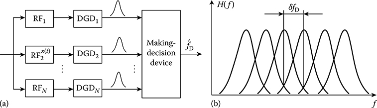
FIGURE 3.21 (a) Doppler frequency measuring by multiple channel filters and (b) amplitude-frequency responses of filters.
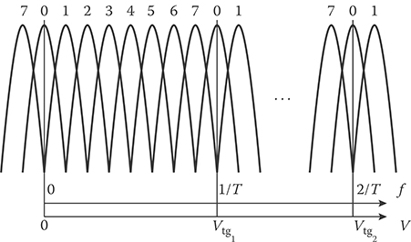
FIGURE 3.22 Amplitude-frequency responses of spectrum analyzer constructed based on DFT, N = 0.
Rough estimation of the Doppler frequency fD can be defined by the channel number with the maximal amplitude of voltage at the measurer output. To increase the accuracy of definition of the Doppler frequency fD estimation we can use the output amplitudes of three frequency channels. In this case, a position of the parabolic amplitude envelope of selected frequency channels is considered as the estimation of the Doppler frequency fD.
Realization in the time domain of the considered filter multiple-channel network is a very difficult problem. For this reason, a realization of the considered filter multiple-channel network in frequency domain based on DFT is of prime interest for us. As well known, the presence of specific spectral characteristic distortions caused by limitation in the sample size N of the input target return signal is a peculiarity of DFT. As a result, the band-pass filter with the central frequency
fk=kNT,k=0,1,…,N−1(3.157)
must correspond to each DFT coefficient. The bandwidth of each filter is equal to N−1. A set of the main lobes of the spectrum analyzer amplitude–frequency response designed and constructed based on DFT at N = 8 are shown in Figure 3.22. Thus, the spectral analyzer designed and constructed based on DFT can be presented as a set of narrowband filters, each of which is the matched filter for sinusoidal signal with frequency matched with the filter central frequency.
The considered features of DFT allow us to employ the corresponding multiple-channel filters to accumulate the coherent target return signals separately in each of N obtained frequency channels. In this case, a detection and estimation of the Doppler frequency of the target return signal is carried out by the number of DFT channels, in which the accumulated signal has exceeded the threshold of detection. If the threshold of detection has been exceeded in several frequency channels, we must make averaging or weight union of frequency estimations of the Doppler frequency. To determine the DFT coefficients, the fast DFT (FDFT) algorithms are used, which allows us to solve the considered problem in real time.
Presence of side lobes in the equivalent amplitude–frequency characteristics of spectral analyzer filters leads us to spectrum splatter (frequency harmonics), and an overlapping of the main lobes forms an incidental amplitude modulation of spectrum. To attenuate the first phenomenon, the specific weight functions called “windows” are used. In using the “window,” DFT takes the following form:
Fuw[k]=N−1∑i=0w[i]u[i]exp{−j2πikN},(3.158)
where
w[i]=w[iT],i=0,1,2,…,N−1(3.159)
is the weight “window” function. In the case of the rectangle weight function, which corresponds practically to DFT of N input signals (the target return signals) without weighting, the side lobes of equivalent amplitude-frequency response of filters are maximal, approximately for about -13 dB. For this reason, as a rule, the “windows” with dropping weight coefficients, for example, triangle, cosine, Gauss, Dolph-Chebyshev, Hamming, and so on, are used.
Under the Doppler frequency estimation, the signal sample size N for DFT is selected to ensure the required spectral resolution
δf=vTN,(3.160)
where v is the coefficient characterizing a spectral bandwidth increase for the selected “window.” As a rule, the value of v is selected equal to an equivalent noise bandwidth of the “window,” that is,
v=∑N−1i=0w2[iT](∑N−1i=0w[iT])2.(3.161)
The incidental amplitude modulation of spectrum leads us to additional losses under signal processing of the target return pulse train, the Doppler frequency of which does not coincide with basic frequencies multiple to the frequency 1/TN. The losses caused by the incidental amplitude modulation of spectrum are for about 1/2 dB in the case of “windows” with smoothly dropping weight coefficients. Maximal losses under DFT caused by maximal losses owing to the incidental amplitude modulation of spectrum for the given “window” and DFT losses caused by a shape of the given “window” do not exceed 3 ÷ 4dB.
3.5 Complex Generalized Algorithms of Digital Interperiod Signal Processing
The complex digital generalized interperiod signal processing/detection algorithm employed by CRSs is offered as a solution to the following problems:
To detect the target return signals
To measure the parameters of target return signals
To form and estimate the current coordinates, parameters, and features of targets by information contained in the target return signals
To code the coordinates and parameters of targets and process them for follow-up processing
The complex digital generalized interperiod signal processing/detection algorithm is synthesized by the composition of particular digital interperiod signal processing/detection algorithms. There are many ways for the composition of the particular digital interperiod signal processing/detection algorithms. The number and content of construction ways of the complex digital generalized interperiod signal processing/detection algorithm depends on the operation conditions of CRSs. At the same time, there is a need to keep in mind that at any condition the CRS operates in very hard noise environment caused by deliberate interferences (active or passive) in conflict situations; reflections from ground objects (buildings, trees, vehicles, mountains, etc.) and atmospheric precipitation (rain, snow, fog, clouds); reflection from non-mechanical objects in atmosphere; and nonsynchronized (chaotic) pulse noise and interference. For this reason, the main problem that is solved in the course of designing the complex digital generalized interperiod signal processing/detection algorithm is the problem of compensation of background and scattering returns and the problem of stabilization of the probability of false alarm PF.
While designing the complex digital generalized interperiod signal processing/detection algorithm it is appropriate to proceed from the assumption that, in each specific case of radar system operation, a definite noise environment requiring reconstruction or retuning of the considered algorithm to ensure a qualitative receiving and processing the target return signals at the fixed probability of false alarm PF will be formed all over the radar coverage or in individual parts of radar coverage. Whereas the number of such situations is very high, we can call several most specific cases:
Signal processing/detection in Gaussian uncorrelated (or weakly correlated) noise with unknown variance
Signal processing/detection in Gaussian uncorrelated (or weakly correlated) noise with unknown variance plus chaotic pulse interference
Signal processing/detection in non-Gaussian noise, for example, while using the intraperiod nonlinear signal processing/detection algorithms (limiters, logarithmic amplifiers, and so on)
Signal processing/detection in correlated Gaussian noise with high variance by value
Under such an approach, naturally, it is required to include the adaptive generalized signal processing/detection algorithms for various noise situations and specific algorithms, which are able to recognize the type of situation and make a decision, into the complex digital generalized interperiod signal processing/detection algorithm. The algorithms recognizing specific situations can be presented in the form of individual signal processing subsystems. Finally, there is a need to provide for a high-speed switchboard in the content of the complex digital generalized interperiod signal processing/detection algorithm, which allows us to carry out all necessary switching in the course of adaptation to noise environment.
Thus, the complex digital generalized interperiod signal processing/detection algorithm for. CRSs must be tuned by the totality of a given set of situations and be adaptive to noise level. The simplest version of the complex digital generalized interperiod signal processing/detection algorithm is shown in Figure 3.23. The subsystem of intraperiod signal processing, the output signals of which are the input signals for the considered complex digital generalized interperiod signal processing/detection algorithm, and the subsystem of environment analysis, the output signals of which are meant for the reconstruction of complex digital generalized interperiod signal processing/detection algorithm, are presented in Figure 3.23 by individual blocks. The following digital signal processing/detection subsystems can be produced by the considered diagram in Figure 3.23:
Digital signal processing and detection subsystem for slowly moving targets and targets moving with blind velocities. The blocks 3, 5, 6, 10, and11 form this subsystem. The block 3 carries out the generation, averaging, and storing of the noise envelope amplitudes for all resolution elements of the CRS. The block 6 generates the thresholds to detect the target return signals at the zero channel output of FDFT filter (the block 5) using the noise envelope amplitudes and omitting the moving-target indicator filter. As a result, there is a greater possibility to detect the target return signals from stationary targets under the condition that the effective reflective surface of target compared to the effective specific surface of passive interference.
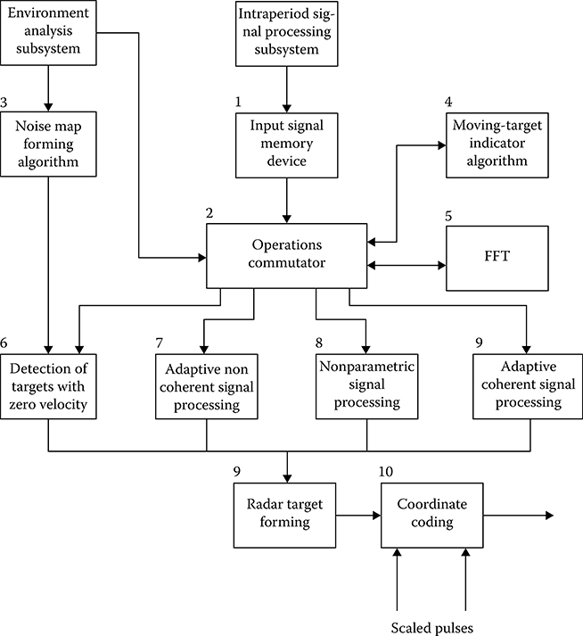
FIGURE 3.23 Simplest version of the complex digital generalized interperiod signal processing/detection algorithm.
No coherent digital adaptive signal processing and detection subsystem formed by cascade connection of the blocks1, 7, 10, and 11. The adapter of decision-making threshold and the target return signal parameter measurer form the block 7.
Nonparametric digital signal processing/detection subsystem formed by the blocks1, 8, 10, and 11. The rank nonparametric digital signal processing/detection algorithm, the adaptive threshold of rank detector, and corresponding detectors and measurers are formed by the block 8.
Coherent adaptive digital signal processing and detection subsystem formed by cascade connection of blocks1,4, 5, 9,10, and 11. Moving-target indication, FDFT of noncompensated remainder samples with the purpose to accumulate target return signals and target radial velocity estimations are realized in this channel. After that, the coherent adaptive signal processing and detection algorithms and estimations of signal parameters are realized in each frequency channel. Owing to the fact of overlapping of frequency channels, the blip operations become essential.
Forming of other signal processing and detection subsystem is possible, for example, coherent signal processing and detection without moving-target indication but with FDFT or without moving-target indication and FDFT, nonparametric digital signal processing and detection with FDFT, and so on.
Final efficacy estimation of considered digital signal processing and detection algorithms is carried out by simulation.
3.6 Summary and Discussion
We summarize briefly the main results discussed in this chapter. The main fundamental theory principles of moving-target indication radar are well discussed in literature. The performance of the moving-target indication radar can be greatly improved due primarily to four advantages: (a) increased stability of radar subsystems such as transmitters, oscillators, and receivers; (b) increased dynamic range of receivers and analog-to-digital converters; (c) faster and more powerful digital signal processing; and (d) better awareness of the limitations, and therefore, requisite solutions of the adapting moving-target indication radar systems to the environment. These four advantages can make it practical to use sophisticated techniques that were considered, and sometimes tried, many years ago but were impractical to implement. Although these developments are able to improve the moving-target indication radar capabilities much more, there are still no perfect solutions to all moving-target indication radar problems, and the design of moving-target indication radar systems is still as much an art as it is a science.
Under the designing and evaluation of efficiency of the digital moving-target indicators, there is a need to take into consideration the following peculiarities: (a) Using the digit capacity Nb ≥ 8 of the target return signal amplitude samples in the digital moving-target indicator, quantization errors can be considered as the white Gaussian noise that is added to the receiver noise; for this reason, a synthesis of the digital moving-target indicator is carried out using an analog prototype, that is, by digitization of well-known analog algorithms. (b) Quantization of the target return signal amplitude samples leads to additional losses at the equalization of passive interferences in comparison with the use of analog moving-target indicators.
In practice, under the evaluation of digital moving-target indicator efficacy the following indices are widely used: (a) the coefficient of interference cancellation Gcan that is defined as a ratio of the input passive interference power to the power of the passive interference at the equalizer output; (b) figure of merit for the case of linear interperiod cancellation of the passive interferences as given by (3.3); in a general case, when a nonlinear signal processing is used, the figure of merit indicates to what extent we can increase an interference power at the equalizer input without decreasing in detection performance; and (c) the coefficient of improvement is a characteristic of the response of digital moving-target indicator on passive interference signals with respect to the averaged response on target return signals. The aforementioned Q-factors can be determined both for equalizer systems for passive interferences using the interperiod subtraction and for equalizer systems with subsequent accumulation of remainders after the passive interference cancellation.
The main element of the digital moving-target indicator is the digital rejector filter that can guarantee a cancellation of correlated passive interference. In the simplest case, the digital filter is constructed in the form of the filter with the v-fold (v ≤ N) interperiod subtraction that corresponds to the structure of nonrecursive filter. The recursive filters are widely used also for cancellation of passive interferences. The digital rejector filter ensures the best cancellation of passive interferences owing to an improvement of the amplitude-frequency characteristic shape in comparison with the nonrecursive rejector filter of the same order. However, there is a higher degree of the correlation of the passive interference remainders at the digital recursive filter output, in comparison with the correlation degree of the passive interference remainders at the digital nonrecursive filter. Moreover, the presence of positive feedback leads to an increase in the time of transient process and corresponding losses in efficacy if the number of target return pulses in the train is less 20, that is, N <20.
Implementation of analog moving-target indicators with the wobble procedure within the limits of the interval T is very difficult since, in this case, there is a need to employ various individual delay circuits for each value of the repetition period T and complex switching system for these circuits. Under realization of the digital moving-target indicator with the wobble procedure within the limits of the interval T, it is enough to realize only the synchronization between a sample of delayed data from memory device and radar searching signal instants. In doing so, the size of memory device does not change and does not depend on the number of discrete values and the wobble procedure function within the limits of the repetition period T. The best speed performance of the digital moving-target indicators with the wobble procedure within the limits of the repetition period T can be obtained if each pulse from the target return pulse train with Ns, where Ns is the number of target return pulses in the train, would be adjusted with a new individual repetition period. The individual repetition period T must be varied with respect to the average value ˉT on the multiple value of fixed time interval ±ΔT. The problem of design and construction of the digital moving-target indicators with the wobble procedure within the limits of the repetition period T is to make a correct selection ˉT of a value T and define the wobble function for pulse train in sequence given by (3.23). In a general case, the wobble procedure is defined by the criterion of the figure of merit η maximization taking into consideration a minimization of amplitude–frequency characteristic ripple in the digital filter bandwidth. As a rule, this problem is solved by simulation methods. Calculations and simulations demonstrate that the wobble procedures for the repetition period T lead to a decrease in the depth of amplitude–frequency response dips of the nonrecursive and recursive digital filters. However, at the same time, a stopband of the nonrecursive and recursive digital filters is narrowed simultaneously with the frequency-band extension and distortion of interference frequency spectrum. For this reason, the effectiveness needed for cancellation of passive interferences is reduced considerably. Absolute losses in the figure of merit η for the recursive digital filters of the second order vary from 0.3 to 4.3 dB and from 4 to 19 dB for the recursive digital filters of the third order in comparison with the digital moving-target indicators without wobble procedures for the repetition period T at optimal velocity.
In practice, spectral-correlation characteristics of passive interferences are unknown a priori and, moreover, heterogeneous in space and nonstationary in time. Naturally, the efficacy of passive interference cancellation is substantially reduced. To ensure high effectiveness of the digital moving-target indication radar subsystems under conditions of a priori uncertainty and nonstationarity of passive interference parameters, the adaptive digital moving-target indication radar subsystems are employed. In a general sense, the problem of adaptive moving-target indication is solved based on an implementation of the correlation feedback principle. Correlation automatic equalizer of passive interferences represents a closed tracker adapting to noise and interference environment without taking into consideration the Doppler frequency. Parallel with high effectiveness, the tracker has a set of the following imperfections: (a) poor cancellation of area-extensive interference leading edge that is a consequence of high time constant value (for about 10 resolution elements) of adaptive feedback; (b) decrease in passive interference cancellation efficiency over the powerful target return signal; and (c) very difficult realization, especially employing digital signal processing. The problem of moving-target indicator adaptation can be solved using the so-called the empirical Bayes approach using of which we at first, define the maximal likelihood estimation (MLE) of passive interference parameters and after that we use these parameters to determine the impulse response coefficients of the rejector digital filter. In this case, we obtain an open-loop adaptation system, the transient process in which is finished within the limits of the digital filter transient process.
Under the discussion of digital signal processing and detection algorithms, we consider two cases, namely, (a) the coherent impulse signals with known parameters and (b) the coherent impulse signals with unknown parameters. In digital signal processing systems, a process of accumulation and signal detection is realized, as a rule, at video frequency after union of in-phase and quadrature channels. In this chapter, we carry out analysis of signal detection problems under the following initial conditions:
The input signal is presented as a single signal, and the signal parameters are the delay td and direction of arrival θ; the total target return signal is a sequence of periodically repeated pulses (the pulse train). As for the statistical characteristics of the target return signal (information signal, i.e., the signal containing information about parameters of the target), we consider two cases: the train of nonfluctuated signals and the train of independently fluctuated signals obeying to the Rayleigh pdf with zero mean and the variance σ2s.
Under synthesis of signal detection algorithms and evaluation of target return signal parameters, we use, as a rule, a noise model in the form of Gaussian random process with zero mean and the variance σ2s; when the correlated in time interferences (namely, passive interferences) are absent, noise samples modeled by the Gaussian process do not have an interperiod correlation; when the passive interferences or their remainders are present after cancellation by the digital moving-target indicators, a sequence of passive interference samples are approximated by Markov chain; to describe statistically the Markov chain we, in addition to the variance, should know the coefficient module ρpi of passive interference interperiod correlation; samples of the input signal Xi in the case of absence of target reflecting surface fluctuations are subjected to the general Rayleigh pdf; in the case of presence of target reflecting surface fluctuations, we can write
p′ℋ1SN(Xi)=Xiσ2Σ+σ2Siexp{−X2i2(σ2Σ+σ2Si)},
where σ2Si is the variance of target return signal amplitude.
A digital signal detection algorithm is considered for two versions: (a) the target return signal is quantized by amplitude in such manner that a low-order bit value does not exceed the root-mean-square value σn of receiver noise. In this case, a stimulus tracking of quantization by amplitude is added up to an addition of independent quantization noise to the input noise and a synthesis of digital signal processing algorithms is reduced to digital realization of optimal analog signal processing algorithms; and (b) the target return signal is quantized on two levels—binary quantization. In this case, there is a need to carry out a direct synthesis of signal processing algorithms and decision devices to process digital binary quantized signals.
Under these conditions, we consider and discuss the following detectors employed by CRSs:
In the case of coherent impulse signals with known parameters,
DGDs for target return pulse train
DGDs for binary quantized target return pulse train
DGDs based on method of the sequential analysis
Software DGDs for binary quantized target return pulse train
In the case of coherent impulse signals with unknown parameters,
Adaptive DGDs
Nonparametric DGDs—sign-nonparametric DGDs and rank-nonparametric DGDs
Adaptive-nonparametric DGDs
Estimation of target return signal parameters comprising information about the coordinates and characteristics of target is the main operation of radar signal preprocessing. Estimation of parameters starts after making the decision a “yes” signal; that is, the target has been detected in direction of scanning at a definite distance. At this time, the target detection is associated with rough calculation of target coordinates, for example, the azimuth accurate with the radar antenna directional diagram width, and the target range accurate with the dimension of resolution element in radar range and so on. The main task of a digital measurer is to obtain more specific information about primary data of estimated target return signal parameters to the predetermined values of target return signal parameters. We investigate algorithms of angular coordinate estimation under uniform and discrete radar antenna scanning. We define the target angular coordinate estimation. In addition, we define the principles of Doppler frequency measurement.
Finally, we suggest and define a structure of the complex digital generalized interperiod signal processing/detection algorithm. While designing the complex digital generalized interperiod signal processing/detection algorithm it is appropriate to proceed from the assumption that, in each specific case of radar system operation, a definite noise environment requiring reconstruction or retuning of the considered algorithm to ensure a qualitative receiving and processing the target return signals at the fixed probability of false alarm PF will be formed all over the radar coverage or in individual parts of radar coverage. Naturally, it is required to include the adaptive generalized signal processing/detection algorithms for various noise situations and specific algorithms, which are able to recognize the type of situation and make a decision, into the complex digital generalized interperiod signal processing/detection algorithm. The algorithms recognizing specific situations can be presented in the form of individual signal processing subsystems. Finally, there is a need to provide for a high-speed switchboard in the content of the complex digital generalized interperiod signal processing/detection algorithm, which allows us to carry out all necessary switching in the course of adaptation to noise environment.
References
1. Skolnik, M. 2008. Radar Handbook. 3rd edn. New York: McGraw-Hills, Inc.
2. Applebaum, S. 1961. Mathematical description of VICI. Report. No. AWCS-EEM-1. Syracuse, NY: General Electric Co.
3. Chow, S.M. 1967. Range and Doppler resolution of a frequency-scanned filter. Proceedings of the IEEE, 114(3): 321–326.
4. Shrader, W.W. 1970. MTI Radar, Chapter 17, in M.I. Skolnik, Ed. Radar Handbook. New York: McGraw-Hills, Inc.
5. Blackman, S. and. R. Popoli. 1999. Design and Analysis of Modern Tracking Systems. Boston, MA: Artech House, Inc.
6. Richards, M.A. 2005. Fundamentals of Radar Signal Processing. New York: John Wiley & Sons, Inc.
7. Barton, D.K. and S.A. Leonov. 1997. Radar Technology Encyclopedia. Norwood, MA: Artech House, Inc.
8. Wehner, D.R. 1995. High Resolution Radar. Norwood, MA: Artech House, Inc.
9. Bozic, S.M. 1994. Digital and Kalman Filtering. 2nd edn. New York: Halsted Press.
10. Brown, R.G. and P.Y.C. Hwang. 1997. Introduction to Random Signals and Applied Kalman Filtering. 3rd edn. New York: John Wiley & Sons, Inc.
11. Diniz, P.S. 1997. Adaptive Filtering. Boston, MA: Kluwer Academic Publisher.
12. Figneiras-Vidal, A.R. Ed. 1996. Digital Signal Processing in Telecommunications. London, U.K.: Springer-Verlag.
13. Grant, P. and B. Mulgrew. 1995. Nonlinear adaptive filter: Design and application, in Proceedings of IFAC on Adaptive Systems in Control and Signal Processing, June 14–16, Budapest, Hungary, pp. 31–42.
14. Haykin, S. 1989. Modern Filters. New York: Macmillan Press, Inc.
15. Johnson, D.H. and D.E. Dudgeon. 1993. Array Signal Processing: Concepts and Techniques. Englewood Cliffs, NJ: Prentice Hall, Inc.
16. Lee, E.A. and. D.G. Messerschmitt. 1994. Digital Communications. 2nd edn. Boston, MA: Kluwer Academic Publisher.
17. Mitra, S.K. 1998. Digital Signal Processing. New York: McGraw-Hills, Inc.
18. Regalia, P.A. 1995. Adaptive IIR Filtering in Signal Processing and Control. New York: Marcel Dekker, Inc.
19. Sayed, A.H. and T. Kailath. 1998. Recursive least-squares adaptive filters, in V. Madisetti, and D. Williams, Eds. The Digital Signal Processing Handbook. New York: CRC Press.
20. Shynk, J.J. 1989. Adaptive IIR filtering. IEEE ASSP Magazine, 6: 4–21.
21. Treichler, J., Johnson, C.R., and M.G. Larimore. 1987. Theory and Design of Adaptive Filters. New York: John Wiley & Sons, Inc.
22. Licharev, V.A. 1973. Digital Techniques and Facilities in Radar. Moscow, Russia: Soviet Radio.
23. Lutovac, M.D., Tosic, D.V., and B.L. Evans. 2001. Filter Design for Signal Processing Using MATLAB and Mathematica. Englewood Cliffs, NJ: Prentice Hall, Inc.
24. Popov, D.I. and V.A. Fedorov. 1975. Efficacy of recursive filters for moving-target indicators. Radio Electronics, 3: 63–68.
25. Wald, A. 1947. Sequential Analysis. New York: John Wiley & Sons, Inc.
26. Glushko, O.V. and L.M. Osynskiy. 1982. Microprocessor for construction of digital filtering systems. Control Systems and Computers, 1: 73–76.
27. Bellanger, M.G. 1987. Adaptive Digital Filters and Signal Analysis. New York: Marcel Dekker, Inc.
28. Purdy, R.J. et al. 2000. Radar signal processing. Lincoln Laboratory Journal, 12(2): 297.
29. Billingsley, J.B. 2002. Low-Angle Radar Land Clutter—Measurements and Empirical Models. Norwich, NY: William Andrew Publishing, Inc.
30. Barton, D.K. 2005. Modern Radar Systems Analysis. Norwood, MA: Artech House, Inc.
31. Skolnik, M.I. 2001. Introduction to Radar Systems. 3rd edn. New York: McGraw-Hills, Inc.
32. Ludloff, A. and M. Minker. 1985. Reliability of velocity measurement by MTD radar. IEEE Transactions on Aerospace and Electronic Systems, 21(7): 522–528.
33. Hall, T.M. and W.W. Shrader. 2007. Statistics of the clutter residue in MTI radars with IF limiting, in IEEE Radar Conference, April 17–20, Boston, MA, pp. 01–06.
34. Cho, J.Y.M. et. al. 2003. Range-velocity ambiguity mitigation schemes for the enhanced terminal Doppler weather radar, in 31st Conference on Radar Meteorology, August 6–12, Seattle, WA, pp. 463–466.
35. Shirman, J.D. and V.H. Manjos. 1981. Theory and Techniques of Radar Signal Processing in Noise. Moscow, Russia: Radio and Svyaz.
36. Popov, D.I. 1981. Synthesis of digital adaptive rejector filters. Radiotechnika, 10: 53–57.
37. Tuzlukov, V. 2010. Multiuser generalized detector for uniformly quantized synchronous CDMA signals in AWGN noise. Telecommunications Review, 20(5): 836–848.
38. Tuzlukov, V. 2011 Signal processing by generalized receiver in DS-CDMA. wireless communication systems with optimal combining and partial cancellation. EURASIP Journal on Advances in Signal Processing, 2011, Article ID.913189: 15, DOI: 10.1155/2011/913189.
39. Tuzlukov, V. 2011. A. Circuits, Systems, and Signal Processing, 30(6): 1197–1230.
40. Tuzlukov, V. 2011. DS-CDMA downlink systems with fading channel employing the generalized receiver. Digital Signal Processing, 21(6): 725–733.
41. Kay, S.M. 1998. Statistical Signal Processing: Detection Theory. Upper Saddle River, NJ: Prentice Hall, Inc.
42. Tuzlukov, V.P. 1998. Signal Processing in Noise: A New Methodology. Minsk, Belarus: IEC.
43. Tuzlukov, V.P. 1998. A new approach to signal detection theory. Digital Signal Processing, 8(3): 166–184.
44. Tuzlukov, V.P. 2001. Signal Detection Theory. New York: Springer-Verlag, Inc.
45. Tuzlukov, V.P. 2002. Signal Processing Noise. Boca Raton, FL: CRC Press.
46. Tuzlukov, V.P. 2005. Signal and Image Processing in Navigational Systems. Boca. Raton, FL: CRC. Press.
47. Tuzlukov, V.P. 2012. Generalized approach to signal processing in wireless communications: The main aspects and some examples. Chapter 11. In Wireless Communications and Networks—Recent Advances, ed. A. Eksim, 305–338. Rijeka, Croatia, IuTech.
48. Tuzlukov, V.P., Yoon, W.S., and Y.D. Kim. 2004. Distributed signal processing with randomized data selection based on the generalized approach in wireless sensor networks. WSEAS Transactions on Computers, 5(3): 1635–1643.
49. Kim, J.H., Kim, J.H., Tuzlukov, V.P., Yoon, W.S., and Y.D. Kim. 2004. FFH and MCFH spread-spectrum wireless sensor network systems based on the generalized approach to signal processing. WSEAS Transactions on Computers, 6(3): 1794–1801.
50. Tuzlukov, V.P., Yoon, W.S., and Y.D. Kim. 2004. Wireless sensor networks based on the generalized approach to signal processing with fading channels and receive antenna array. WSEAS Transactions on Circuits and Systems, 10(3): 2149–2155.
51. Kim, J.H., Tuzlukov, V.P., Yoon, W.S., and Y.D. Kim. 2005. Performance analysis under multiple antennas in wireless sensor networks based on the generalized approach to signal processing. WSEAS Transactions on Communications, 7(4): 391–395.
52. Kim, J.H., Tuzlukov, V.P., Yoon, W.S., and Y.D. Kim. 2005. Macrodiversity in wireless sensor networks based on the generalized approach to signal processing. WSEAS Transactions on Communications, 8(4): 648–653.
53. Kim, J.H., Tuzlukov, V.P., Yoon, W.S., and Y.D. Kim. 2005. Generalized. detector under no orthogonal multipulse modulation in remote sensing systems. WSEAS Transactions on Signal Processing, 2(1): 203–208.
54. Tuzlukov, V.P. 2009. Optimal combining, partial cancellation, and channel estimation and correlation in. DS-CDMA systems employing the generalized detector. WSEAS Transactions on Communications, 7(8): 718–733.
55. Tuzlukov, V.P., Yoon, W.S., and Y.D. Kim. 2004. Adaptive beam-former generalized detector in wire-less sensor networks, in Proceedings of IASTED International Conference on Parallel and Distributed Computing and Networks (PDCN 2004), February 17–19, Innsbruck, Austria, pp. 195–200.
56. Tuzlukov, V.P., Yoon, W.S., and Y.D. Kim. 2004. Network assisted diversity for random access wireless sensor networks under the use of the generalized approach to signal processing, in Proceedings of the 2nd SPIE International Symposium on Fluctuations in Noise, May 25–28, Maspalomas, Gran Canaria, Spain, Vol. 5473, pp. 110–121.
57. Tuzlukov, V.P., Yoon, W.S., and. Y.D. Kim. 2005. MMSE multiuser generalized detector for no orthogonal multipulse modulation in wireless sensor networks, in Proceedings of the 9th World Multiconference on Systemics, Cybernetics, and Informatics (WMSCI 2005), July 10–13, Orlando, FL (CD Proceedings)
58. Kim, J.H., Tuzlukov, V.P., Yoon, W.S., and Y.D. Kim. 2005. Collaborative wireless sensor networks for target detection based on the generalized approach to signal processing, in Proceedings of International Conference on Control, Automation, and Systems (ICCAS 2005), June 2–5, Seoul, Korea. (CD. Proceedings)
59. Tuzlukov, V.P., Chung, K.H., and Y.D. Kim. 2007. Signal detection by generalized detector in compound-Gaussian noise, in Proceedings of the 3rd WSEAS International Conference on Remote Sensing (REMOTE’07), November 21–23, Venice (Venezia), Italy, pp. 1–7.
60. Tuzlukov, V.P. 2008. Selection of partial cancellation factors in DS-CDMA systems employing the generalized detector, in Proceedings of the 12th WSEAS International Conference on Communications, July 23–25, Heraklion, Creete, Greece. (CD Proceedings)
61. Tuzlukov, V.P. 2008. Multiuser generalized detector for uniformly quantized synchronous CDMA signals in wireless sensor networks with additive white Gaussian noise channels in Proceedings of the International Conference on Control, Automation, and Systems (ICCAS 2008), October 14–17, Seoul, Korea. pp. 1526–1531.
62. Tuzlukov, V.P. 2009. Symbol error rate of quadrature subbranch hybrid selection/maximal-ratio combining in Rayleigh fading under employment of generalized detector, in Recent Advances in Communications: Proceedings of the 13th WSEAS International Conference on Communications, July 23–25, Rodos (Rhodes) Island, Greece, pp. 60–65.
63. Tuzlukov, V.P. 2009. Generalized detector with linear equalization for frequency-selective channels employing finite impulse response beamforming, in Proceedings of the 2nd International Congress on Image and Signal Processing (CISP 2009), October 17–19, Tianjin, China, pp. 4382–4386.
64. Tuzlukov, V.P. 2010. Optimal waveforms for MIMO radar systems employing the generalized detector in Proceedings of the International Conference on Sensor Data and Information Exploitation: Automatic Target Recognition, Part of the SPIE International Symposium on Defense, Security, and Sensing, April 5–9, Orlando, FL, Vol. 7697, pp. 76971G-1–76971G-12.
65. Tuzlukov, V.P. 2010. MIMO radar systems based on the generalized detector and space-time coding, in Proceedings of the International Conference on Sensor Data and Information Exploitation: Automatic Target Recognition, Part of the SPIE International Symposium on Defense, Security, and Sensing, April. 5–9, Orlando, FL, Vol. 7698, pp. 769805-1–769805-12.
66. Tuzlukov, V.P. 2010. Generalized receiver under blind multiuser detection in wireless communications, in Proceedings of IEEE International Symposium on Industrial Electronics (ISIE 2010), July 4–7, Bari, Italy, pp. 3483–3488.
67. Khan, R.R. and V.P. Tuzlukov. 2010. Multiuser data fusion algorithm for estimation of a walking person position, in Proceedings of International Conference on Control, Automation, and Systems (ICCAS 2010), October 27–30, Seoul, Korea. pp. 863–867.
68. Khan, R.R. and V.P. Tuzlukov. 2010. Beamforming for rejection of co-channels interference in an OFDM system, in Proceedings of the 3rd International Congress on Image and Signal Processing (CISP 2010), October 16–18, Yantai, China. pp. 3318–3322.
69. Khan, R.R. and V.P. Tuzlukov. 2010. Null-steering beamforming for cancellation of co-channel interference. in CDMA wireless communications systems, in Proceedings of the 4th IEEE International Conference on Signal Processing and Communications Systems (ICSPCS’2010), December 13–15, Goald Coast, Queensland, Australia. (CD Proceedings).
70. Akimov, P.S., Bacut, P.A., Bogdanovich, V.A. et al. 1984. Theory of Signal Detection. Moscow, Russia: Radio and Svyaz.
71. Wald, A. 1950. Statistical Decision Functions. New York: John Wiley & Sons, Inc.
72. Fu, K. 1968. Sequential Methods in Pattern Recognition and Machine Learning. New York: Academic. Press.
73. Ghosh, B. 1970. Sequential Tests of Statistical Hypotheses. Cambridge, MA: Addison-Wesley.
74. Siegmund, D. 1985. Sequential Analysis: Tests and Confidence Intervals. New York: Springer-Verlag.
75. Wald, A. and. J. Wolfowitz. 1948. Optimum. character of the sequential probability ratio test. Annual Mathematical Statistics, 19: 326–339.
76. Aarts, E.H.L. 1989. Simulated Annealing and Boltzman Machines: A Stochastic Approach to Combinational Optimization and Neural Computing. New York: John Wiley & Sons, Inc.
77. Blahut, R.E. 1987. Principles and Practice of Information Theory. Reading, MA: Addison-Wesley.
78. Kuzmin, S.Z. 1967. Digital Signal Processing in Radar. Moscow, Russia: Soviet Radio.
79. Eaves, J.L. and E.K. Reedy. 1987. Principles of Modern Radar. New York: Van Nostrand Reinhold.
80. Edde, B. 1995. Radar: Principles, Technologies, Applications. Upper Saddle River, NJ: Prentice Hall, Inc.
81. Levanon, N. 1988. Radar Principles. New York: John Wiley & Sons, Inc.
82. Peebles, Jr. P.Z. 1998. Radar Principles. New York: John Wiley & Sons, Inc.
83. Alexander, S.T. 1986. Adaptive Signal Processing: Theory and Applications. New York: Springer-Verlag.
84. Clarkson, P.M. 1993. Optimal and Adaptive Signal Processing. Boca Raton, FL: CRC Press.
85. Pitas, I. and A.N. Wenetsanopoulos. 1990. Nonlinear Digital Filters. Boston, MA: Kluwer Academic Publishers.
86. Sibal, L.H., Ed. 1987. Adaptive Signal Processing. New York: IEEE Press.
87. Widrow, B. and S. Stearns. 1985. Adaptive Signal Processing. Englewood Cliffs, NJ: Prentice Hall, Inc.
88. Lacomme, P., Hardange, J.P., Marchais, J.C., and E. Normant. 2001. Air and Spaceborne Radar Systems. Norwich, NY: William Andrew Publishing, LLC.
89. Bakulev, P.A. and V.M. Stepin. 1986. Methods and Hardware of Moving-Target Indication. Moscow, Russia: Radio and Svyaz.
90. Sherman, S.M. 1986. Monopulse Principles and Techniques. Norwood, MA: Artech House, Inc.
91. Leonov, A.I. and K.I. Formichev. 1986. Monopulse Radar. Norwood, MA: Artech House, Inc.