Chapter 7 Design Principles of Complex Algorithm Computational Process in Radar Systems

Search in book...
Toggle Font Controls
Create new playlist

Name your new playlist

Playlist description (optional)
Sign In

Email address

Password

Forgot Password?

or

Continue with Facebook

Continue with Google
Sign Up

Full Name

Email address

Confirm Email Address

Password

or

Continue with Facebook

Continue with Google

The exponential growth in digital technology since the 1980s, along with the corresponding decrease in its cost, has had a profound impact on the way radar systems are designed. More and more functions that were historically implemented in analog hardware are now being performed digitally, resulting in increased performance and flexibility and reduced size and cost. Advances in analog-to-digital converter (ADC) and digital-to-analog converter (DAC) technologies are pushing the border between analog and digital processing closer and closer to the antenna. For example, Figure 7.1 shows a simplified flowchart of the receiver front end of a typical radar system that would have been designed around 1990. Note that this system incorporated analog pulse compression (PC). It also included several stages of analog downconversion in order to generate baseband in phase (I) and quadrature (Q) signal components with a small enough bandwidth so that the ADCs of the day could sample them. The digitized signals were then fed into digital Doppler/moving target indicator (MTI) and detection processors.

By contrast, Figure 7.2 depicts a typical digital receiver for a radar front end. The radio frequency (RF) input usually passes through one or two stages of analog downconversion to generate an intermediate frequency (IF) signal that is sampled directly by the ADC A digital downconverter (DDC) converts the digitized signal samples to complex form at a lower rate for passing through a digital pulse compressor to backend processing. Note that the output of the ADC has a slash through the digital signal line with a letter provided earlier. The letter depicts the number of bits in the digitized input signal and represents the maximum possible dynamic range of the ADC The use of digital signal processing (DSP) can often improve the dynamic range, stability, and overall performance of the system, while reducing size and cost, compared with the analog approach.

7.1 Design Considerations

In coherent radar systems, all local oscillators (LOs) and clocks that generate system timing are derived from a single reference oscillator. However, this fact alone does not ensure that the transmitted waveform starts at the same RF phase on every pulse, which is a requirement for coherent systems. Consider a system with a 5 MHz reference oscillator, from which is derived a 75 MHz IF center frequency (on transmit and receive) and a complex sample rate of 30 MHz. A rule of thumb is that the clock used to produce the pulse repetition interval (PRI) needs to be a common denominator of the IF center frequencies on transmit and receive and the complex sample frequency in order to assure pulse-to-pulse phase coherency. For this example, with an IF center frequency of 75 MHz and a complex sample rate of 30 MHz, allowable PRI clock frequencies would include 15 and 5 MHz.

In the past, implementing a real-time radar digital signal processor typically required the design of a custom computing machine, using thousands of high-performance integrated circuits (ICs) These machines were very difficult to design, develop, and modify Digital technology has advanced to the point where several implementation alternatives exist that make the processor more programmable and easier to design and change.

Images

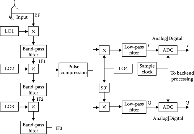
FIGURE 7.1 Typical radar receiver front end design from 1990.

Images

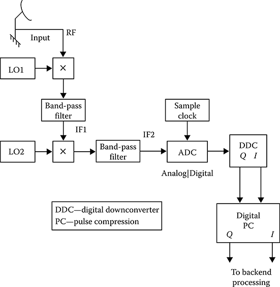
FIGURE 7.2 Typical digital receiver front end.

7.1.1 PARALLEL GENERAL-PURPOSE COMPUTERS

This architecture employs multiple general-purpose processors that are connected via high-speed communication networks. Included in this class are high-end servers and embedded processor architectures. Servers are typically homogeneous processors, where all of the processing nodes are identical and are connected by a very high-performance data bus architecture Embedded processor architectures are typically composed of single-board computers (blades) that contain multiple general-purpose processors and plug into standard backplane architecture. This configuration offers the flexibility of supporting a heterogeneous architecture, where a variety of different processing blades or interface boards can be plugged into the standard backplane to configure a total system. At this writing, backplanes are migrating from parallel architectures, where data are typically passed as 32 or 64 bit words, to serial data links, which pass single bits at very high clock rates (currently in excess of 3 GB/s [GBps]). These serial data links are typically point-to-point connections. In order to communicate with multiple boards, the serial links from each board go to a high-speed switchboard that connects the appropriate source and destination serial links together to form a serial fabric. It is apparent that high-speed serial links will be the primary communication mechanism for multiprocessor systems in the future, with ever-increasing data bandwidths. These parallel processor architectures offer the benefit of being programmable using high-level languages, such as C and C++. A related advantage is that programmers can design the system without knowing the intimate details of the hardware In addition, the software developed to implement the system can typically be moved relatively easily to new hardware architecture as part of a technology refresh cycle.

On the negative side, these systems can be difficult to program to support real-time signal processing. The required operations need to be split up appropriately among the available processors, and the results need to be properly merged to form the final result. A major challenge in these applications is to support the processing latency requirements of the system, which define the maximum length of time allowed to produce a result The latency of the microprocessor system is defined as the amount of time required to observe the effect of a change at a processor’s input on its output. Achieving latency goals often requires assigning smaller pieces of the workload to individual processors, leading to more processors and a more expensive system Another challenge facing these systems in radar application is reset time In a military application, when a system needs to be reset in order to fix a problem, the system needs to come back to full operation in a very short period of time These microprocessor systems typically take a long time to reboot from a central program store and, hence, have difficulty meeting reset requirements. Developing techniques to address these deficiencies is an active area of research. Finally, these processors are generally used for nonreal time or near-real time data processing, as in target tracking and display processing. Since the 1990s, they have started to be applied to real-time signal processing applications. Although they might be cost-effective for relatively narrowband systems, their use in wideband DSP systems in the early twenty-first century is typically prohibitively expensive due to the large number of processors required This situation should improve over time as faster and faster processors become available.

7.1.2 CUSTOM-DESIGNED HARDWARE

Through the 1990s, real-time radar DSP systems were built using discrete logic These systems were very difficult to develop and modify, but in order to achieve the required system performance, it was the only option available. Many radar systems were built using application-specific integrated circuits (ASICs), which are custom devices designed to perform a particular function. The use of ASICs allowed DSP systems to become very small with high performance. However, they were (and still are) difficult and expensive to develop, often requiring several design interactions before the device was fully operational. If an ASIC-based system needs to be modified, the ASICs need to be redesigned, incurring significant expense. Typically, the use of ASICs makes sense if tens or hundreds of thousands of units are to be sold, so that the development costs can be amortized over the life of the unit. This is rarely the case for radar systems However, many ASICs have been developed to support the communication industry, such as digital up- and downconverter, which can be utilized in radar systems.

The introduction of the field programmable gate array (FPGA) in the 1980s heralded a revolution in the way real-time DSP systems were designed FPGAs are integrated circuits that consist of a large array of configurable logic elements that are connected by a programmable interconnect structure At the time of this writing, FPGAs can also incorporate hundreds of multipliers that can be clocked at rates up to a half billion operations per second, and memory blocks, microprocessors, and serial communication links that can support multigigabit-per-second data transfers. Circuits are typically designed using a hardware description language (HDL), such as VHDL (VHSIC hardware description language) or Verilog. Software tools convert this high-level description of the processor to a file that is sent to the device to tell it how to configure itself. High-performance FPGAs store their configuration in volatile memory, which loses its contents when powered down, making the devices infinitely reprogrammable.

FPGAs allow the designer to fabricate complex signal processing architectures very efficiently. In typical large applications, FPGA-based processors can be a factor of 10 (or more) smaller and less costly than systems based on general-purpose processors This is due to the fact that most microprocessors only have one or few processing elements, whereas FPGA have an enormous number of programmable logic elements and multipliers. For example, to implement a 16 tap FIR filter in a microprocessor with a single multiplier and accumulator, it would take 16 clock cycles to perform the multiplications In an FPGA, we could assign 16 multipliers and 16 accumulators to the task, and the filter could be performed in 1 clock cycle In order to use an FPGA most efficiently, we have to take advantage of all of the resources it offers These include not only the large numbers of logic elements, multipliers, and memory blocks but also the rate at which the components can be clocked In the previous example, assume that the data sample rate is 1 MHz and also assume that the multipliers and logic can be clocked at 500MHz. If we simply assign one multiplier to each coefficient, we would use 16 multipliers clocking at 500MHz. Since the data rate is only 1 MHz, each multiplier would only perform one significant multiplication every microsecond and then be idle for the other 499 clocks in the microsecond, which is very inefficient It would be much more efficient, in this case, to use one multiplier to perform as many products as possible. This technique, called time-domain multiplexing, requires additional logic to control the system and provide the correct operands to the multiplier at the right time Since an FPGA can incorporate hundreds of multipliers, one can appreciate the power of this technique.

On the negative side, utilizing an FPGA to its best advantage typically requires the designer to have a thorough understanding of the resources available in the device This typically makes efficient FPGA-based systems harder to design than radar systems based on general-purpose processors, where a detailed understanding of the microprocessor system architecture is not necessarily required In addition, FPGA designs tend to be aimed at a particular family of devices and take full advantage of the resources provided by that family Hardware vendors are constantly introducing new products, invariably incorporating new and improved capabilities Over time, the older devices become obsolete and need to be replaced during a technology refresh cycle. When a technology refresh occurs several years down the road, typically the available resources in the latest FPGAs have changed or a totally different device family is used, which probably requires a redesign On the other hand, software developed for general-purpose processors may only need to be recompiled in order to move it to a new processor. Tools currently exist that synthesize C or MATLAB® code into an FPGA design, but these tools are typically not very efficient The evolution of design tools for FPGAs to address these problems is an area of much research and development.

Hybrid processors: Although it would be very desirable to simply write C code to implement a complex radar signal processor, the reality in the early twenty-first century is that, for many radar systems, implementing such a system would be prohibitively expensive or inflict major performance degradation Although the steady increase in processor throughput may someday come to the rescue, the reality at the time of writing is that high-performance radar signal processors are usually a hybrid of application-specific and programmable processors. Dedicated processors, such as FPGAs or ASICs, are typically used in the high-speed front end of radar signal processors, performing demanding functions such as digital downconversion and pulse compression, followed by programmable processors in the rear, performing the lower-speed tasks such as detection processing The location of the line that separates the two domains is application-dependent, but over time, it is constantly moving toward the front end of the radar system.

7.2 Complex Algorithm Assignment

The complex algorithm of a computational process is a set of elementary DSP algorithms for all stages and complex radar system (CRS) modes of operation. Off-line complex algorithms of DSP individual stages that are not associated with each other by information processes and control operations are possible, too. To design the complex algorithm of a computational process, there is a need to have an unambiguous definition of microprocessor system functioning under solution of goal-oriented DSP problems This definition must include the elementary DSP and control algorithms, a sequence of their application, the conditions of implementation of each elementary DSP and control algorithm, and intercommunication between the DSP and control algorithms using input and output information. A general form of such definition and description can be presented using the logical and graph flowchart of the DSP and control algorithms.

The complex algorithm can be realized by a multiprocessor system. In this case, the elementary operations are distributed among the microprocessors taking into consideration their operation speed, and the complex algorithm must be transformed into the form suitable for realization in parallel microprocessor systems (parallelization of the complex algorithm) The method of algorithmic representation and transformation is the subject of investigation in the theory of algorithms.

7.2.1 LOGICAL AND MATRIX ALGORITHM FLOWCHARTS

Universal ways of algorithm assignment are designed by the theory of algorithms. At that time, any general way to assign the complex algorithms is based on the dual character objects, namely, the counting operators and the logical operators (or recognizers). In our case, the counting operators A₁, A₂, ..., are the elementary DSP algorithms. The logical operators (recognizers) P_j, P₂, ..., P_i are used to recognize some features of information processed by the complex DSP algorithm and to change a sequence of elementary algorithms depending on results of recognition.

One of the best-known ways to assign the complex DSP algorithm depending on complexity is the logical or formula-logical algorithmic flowchart The elementary operators and recognizers are presented in the geometrical form in the logical algorithm flowchart (rectangle, jewel boxes, trapeziums, etc ) connected with each other by arrows in accordance with the given sequence of counting operators and recognizers in the complex algorithm. Titles of elementary operations (DSP algorithms) are written inside the geometrical forms Sometimes the formulas of logical operations carried out and logical conditions under test are written inside the geometrical forms In this case, the corresponding logical flowchart of the complex DSP algorithm is called the formula-logical block diagram.

The complex algorithm can be presented also by operator diagram consisting of elementary counting operators (the elementary DSP algorithms), recognizers, and indicators to carry out operations in sequence. Additionally, we use the specific operators to start A₀ and to stop A_k. For example, we can design the following operator diagram of algorithms based on the counting operators A₁, A₂, A₃, A₄, and A₅ and recognizers P₁, P₂, P₃, and P₄:

A 0 ↓ 3 A 1 P 1 ↑ 1 A 2 P 2 ↑ 2 ↓ 1 P 3 ↑ 3 A 3 ↓ 2 A 4 P 4 ↑ 4 A s ↓ 4 A k, (7.1)

$A_{0} \overset{3}{↓} A_{1} P_{1} \overset{1}{↑} A_{2} P_{2} \overset{2}{↑} \overset{1}{↓} P_{3} \overset{3}{↑} A_{3} \overset{2}{↓} A_{4} P_{4} \overset{4}{↑} A_{s} \overset{4}{↓} A_{k}, (7.1)$

where

↑ means the arrow beginning
↓ means the arrow end

The beginning and the end of the same arrow are designated by the same number The algorithm starts to work after using the operator A₀ “Start.” The order to work for other blocks of the operational flowchart is the following. If the last active block is the counting operator, then the next in step-by-step block works. If the last active block is the recognizer, then two cases are possible. If the test condition is satisfied, then the neighbor at the right side block works. If the test condition is not satisfied, then the block marked by the arrow directed from the recognizer works. The algorithm stops working if the last active operator possesses an assignment to pass to the operator A_k “Stop.” The operator flowcharts of algorithms are very compact but not so obvious and require additional explanations and the operator sense decoding.

To write the order of the elementary DSP algorithms functioning as components of the complex algorithm, we use the matrix form:

A = A 0 A 1 A 2 ⋮ A n A 1 α 01 α 11 α 21 \dots α n 1 A 2 α 02 α 12 α 22 \dots α n 2 \dots \dots \dots \dots \dots \dots A n α 0 n α 1 n α 2 n \dots α n n A k α 0 k α 1 k α 2 k \dots α n k, (7.2)

$A = \begin{array}{l} A_{1} & A_{2} & \dots & A_{n} & A_{k} \\ A_{0} & α_{01} & α_{02} & \dots & α_{0 n} & α_{0 k} \\ A_{1} & α_{11} & α_{12} & \dots & α_{1 n} & α_{1 k} \\ A_{2} & α_{21} & α_{22} & \dots & α_{2 n} & α_{2 k} \\ ⋮ & \dots & \dots & \dots & \dots & \dots \\ A_{n} & α_{n 1} & α_{n 2} & \dots & α_{n n} & α_{n k} \end{array}, (7.2)$

where

α i j = α i j (P 1, P 2, \dots, P l), i = 0, 1, 2, \dots, n; j = 1, 2, \dots, n, n + 1 (7.3)

$α_{i j} = α_{i j} (P_{1}, P_{2}, \dots, P_{l}), i = 0, 1, 2, \dots, n; j = 1, 2, \dots, n, n + 1 (7.3)$

are the logical functions satisfying the following condition: if after the algorithm A. performance the function α_ij at some set of the logical elements P₁, P₂, ..., P₁ taking magnitudes P_i = 1 or Pi¯¯¯ = 0 $\bar{P_{i}} = 0$ is equal to unit, then the algorithm A_j must be the next to operate. If some functions α_ij = 1, then the algorithm A_j must operate after the algorithm A_i. Conversely, if some functions αij ≡ 0, then under realization of the complex algorithm the operation of the elementary algorithm A_j is impossible after operation of the elementary algorithm A_i. The matrix flowchart of the operator algorithm given by (7.1) takes the following form:

A = A 0 A 1 A 2 A 3 A 4 A 5 A 1 1 P 1 ¯ ¯ ¯ ¯ P 3 ¯ ¯ ¯ ¯ P 2 P 3 ¯ ¯ ¯ ¯ 000 A 2 0 P 1 0000 A 3 0 P 1 ¯ ¯ ¯ ¯ P 3 P 2 P 3 000 A 4 00 P 2 ¯ ¯ ¯ ¯ 100 A s 0000 P 4 0 A k 0000 P 4 ¯ ¯ ¯ ¯ 1 . (7.4)

$A = \begin{array}{l} A_{1} & A_{2} & A_{3} & A_{4} & A_{s} & A_{k} \\ A_{0} & 1 & 0 & 0 & 0 & 0 & 0 \\ A_{1} & \bar{P_{1}} \bar{P_{3}} & P_{1} & \bar{P_{1}} P_{3} & 0 & 0 & 0 \\ A_{2} & P_{2} \bar{P_{3}} & 0 & P_{2} P_{3} & \bar{P_{2}} & 0 & 0 \\ A_{3} & 0 & 0 & 0 & 1 & 0 & 0 \\ A_{4} & 0 & 0 & 0 & 0 & P_{4} & \bar{P_{4}} \\ A_{5} & 0 & 0 & 0 & 0 & 0 & 1 \end{array} . (7.4)$

Let notation A_i → A_j mean that after the algorithm A_i operation there is a need to carry out the algorithm A_j Then the notation.

A j \to α i 1 A 1 + α i 2 A 2 + \dots + α i n A n (7.5)

$A_{j} \to α_{i 1} A_{1} + α_{i 2} A_{2} + \dots + α_{i n} A_{n} (7.5)$

means that the operation of one of those algorithms with the functions α_ij ≠ 0 is possible after the algorithm A_i operation. Equation 7.5 is called the transition formula for the algorithm A_i. These formulas can be designed for all elementary DSP algorithms of the complex algorithm given by the matrix flowchart. Thus, in the case of matrix form (7.4), we obtain the following system of transition formulas:

⎧ ⎩ ⎨ ⎪ ⎪ ⎪ ⎪ ⎪ ⎪ ⎪ ⎪ ⎪ ⎪ ⎪ ⎪ ⎪ ⎪ ⎪ ⎪ ⎪ ⎪ A 0 A 1 A 2 A 3 A 4 A 4 \to \to \to \to \to \to A 1; P 1 ¯ ¯ ¯ ¯ P 3 ¯ ¯ ¯ ¯ A 1 + P 1 ¯ ¯ ¯ ¯ A 2 + P 1 ¯ ¯ ¯ ¯ P 3 A 3; P 2 P 3 ¯ ¯ ¯ ¯ A 1 + P 2 P 3 A 3 + P 2 ¯ ¯ ¯ ¯ A 4; A 4; P 4 A s + P 4 ¯ ¯ ¯ ¯ A k; A k . (7.6)

${\begin{array}{l} A_{0} & \to & A_{1}; \\ A_{1} & \to & \bar{P_{1}} \bar{P_{3}} A_{1} + \bar{P_{1}} A_{2} + \bar{P_{1}} P_{3} A_{3}; \\ A_{2} & \to & P_{2} \bar{P_{3}} A_{1} + P_{2} P_{3} A_{3} + \bar{P_{2}} A_{4}; \\ A_{3} & \to & A_{4}; \\ A_{4} & \to & P_{4} A_{s} + \bar{P_{4}} A_{k}; \\ A_{4} & \to & A_{k} . \end{array} (7.6)$

The matrix flowchart of the complex algorithm allows us to design the table reflecting both information and controlling association between the elementary DSP algorithms. We may change all the matrix elements by magnitudes.

l i j = {1, 0, i f i f α i j \neq 0 i n (7.2); α i j = 0 i n (7.2) . (7.7)

$l_{i j} = {\begin{array}{l} 1, & i f & α_{i j} \neq 0 i n (7.2); \\ 0, & i f & α_{i j} = 0 i n (7.2) . \end{array} (7.7)$

As a result, we obtain the adjacency matrix that reflects formally an information association between the elementary DSP algorithms. For instance, the algorithm given by the matrix in (7.4) has the following adjacency matrix:

A = A 0 A 1 A 2 A 3 A 4 A 5 A 1 111000 A 2 010000 A 3 011000 A 4 001100 A 5 000010 A k 000011 . (7.8)

$A = \begin{array}{l} A_{1} & A_{2} & A_{3} & A_{4} & A_{5} & A_{k} \\ A_{0} & 1 & 0 & 0 & 0 & 0 & 0 \\ A_{1} & 1 & 1 & 1 & 0 & 0 & 0 \\ A_{2} & 1 & 0 & 1 & 1 & 0 & 0 \\ A_{3} & 0 & 0 & 0 & 1 & 0 & 0 \\ A_{4} & 0 & 0 & 0 & 0 & 1 & 1 \\ A_{5} & 0 & 0 & 0 & 0 & 0 & 1 \end{array} . (7.8)$

We can design the graph flowchart of the complex algorithm of computational process based on the adjacency matrix.

7.2.2 ALGORITHM GRAPH FLOWCHARTS

The algorithm graph flowchart is the finite oriented graph satisfying the following conditions:

There are two marked nodes in the graph: the input node corresponds to the operator “Start” and the only arrow is directed from this operator; and the output node corresponds to the operator “Stop” and no arrow is directed from this node.
One arrow (the node A) or two arrows (the node P) are directed from each node excepting the input and output nodes; the arrows from the node P are marked by the signs “+” and “-” or by the digits “1” and “0.”
The elementary DSP algorithm A_i is correlated with the A-node and the logical operator P_l is matched with each P-node; in the algorithm graph flowcharts, the A-nodes and the input and output nodes are depicted by circles and the P-nodes are depicted by jewel boxes.

The algorithm graph flowchart i.e., equivalent to the given matrix flowchart, i.e., with the same operation sequence, is designed in the following way:

The subgraphs equivalent to transition formulas of the given matrix flowchart are designed.
The equivalent branches of subgraphs are united.
The same operators are united and the final graph flowchart is formed.

To obtain the graph flowchart with the minimal or near minimum number of P-nodes, there is a need to draw the subgraphs with the minimum number of P-nodes, too, using the given transition formulas The number of P-nodes can be reduced under union of the equivalent subgraph branches The procedure to design and transform the algorithm graph flowchart can be illustrated by an example considering the matrix flowchart of algorithm given by (7.4) as the initial form. The transition formulas given by (7.6) are initial to design the graph flowchart, based on which the subgraphs for each elementary DSP algorithms A₀, A₁, A₂, A₃, A₄, A₅ must be drawn. The subgraph design process is started from the transition formula transformation to the corresponding form consisting of logical function expansion with respect to each variable. For example, the transition formula for the elementary DSP algorithm A _jgiven by (7 6) takes the following form:

A 1 \to P 1 A 2 + P ¯ ¯ ¯ 1 (P 3 A 3 + P ¯ ¯ ¯ 3 A 1) . (7.9)

$A_{1} \to P_{1} A_{2} + {\bar{P}}_{1} (P_{3} A_{3} + {\bar{P}}_{3} A_{1}) . (7.9)$

The formula for the elementary DSP algorithm A₂ given by (7.6) takes the following form:

A 2 \to P 2 (P 3 ¯ ¯ ¯ ¯ A 1 + P 3 A 3) + P ¯ ¯ ¯ 2 A 4 . (7.10)

$A_{2} \to P_{2} (\bar{P_{3}} A_{1} + P_{3} A_{3}) + {\bar{P}}_{2} A_{4} . (7.10)$

Other transition formulas given by (7.6) do not require representation. Now, it is easy to draw the subgraphs of each elementary DSP algorithm (see Figure 7.3).

The next stage is the search and union of equivalent graph branches. In our case, the equivalent branches are the branches starting from the operator P circled by the dash line. After union of the equivalent branches, we obtain the subgraph depicted in Figure 7.4. There are no other equivalent branches for the considered example. Finally, after union of the same counting operators, we obtain the end graph flowchart of algorithm equivalent to the given matrix block diagram (see Figure 7.5). The considered example to design the graph flowchart by the given matrix block diagram allows us to minimize the number of logical operators of complex algorithm, which means to simplify it. The stage of minimization of the operator numbers is the necessary stage for DSP.

Images

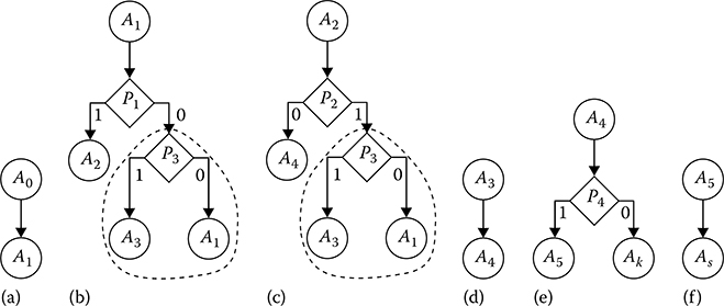
FIGURE 7.3 Subgraphs of each elementary DSP algorithm: (a) the algorithm A₀; (b) the algorithm A_j; (c) the algorithm A₂; (d) the algorithm A₃; (e) the algorithm A₄; and (f) the algorithm A₅.

Images

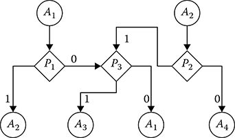
FIGURE 7.4 The subgraph uniting equivalent branches.

Images

FIGURE 7.5 Final graph flowchart equivalent to the given matrix diagram.

Under analysis of features and quality of algorithms presented by the graph flowcharts, it is worthwhile to transform them further with the purpose of uniting the elementary DSP algorithm with the logical operators (in pairs or some elementary DSP algorithm with a single logical operator) into nodes that are used for realization more or less components of the complex algorithm Two arrows come out from such united node: if the test condition is satisfied as a result of node operation, the arrow is denoted by the sign “+” or “1,” otherwise by the sign “-” or “0.” For instance, in the case of the algorithm with flowchart presented in Figure 7.5, we can unite the algorithms into blocks (the input and output nodes are not united): a₁ ˜ A₁PP₁, a₂ ~ A₂P₂, a₃ ~ P₃, a₄ ~ A₁P₁, a₁ ~ A₄P₄, a₅ ~ A₃A₄P₄, a₆= A₅. The obtained flowchart is depicted in Figure 7.6, where the nodes are designated by the light circles.

Images

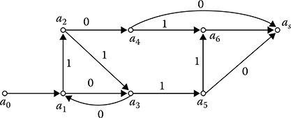
FIGURE 7.6 Union of algorithms into blocks.

7.2.3 USE OF NETWORK MODEL FOR COMPLEX ALGORITHM ANALYSIS

The main problem solved by the graph flowcharts of complex DSP algorithms is a definition of rational ways to present these problems and a choice of computational software tools and microprocessor subsystems to realize the complex DSP algorithm of a radar system. In short, the problem of optimization of computational process is assigned The solution of this problem allows us to reduce significantly a realization time and to simplify the complex DSP algorithm of the radar system Similar problems are the problems of network planning and control [1,2].

To design the network model of computational process under DSP in CRSs, there is a need to transform the graph flowchart of complex algorithm into the network graph that satisfies the following requirements, namely, the network graph cannot consist of contours, that is, the case when the initial top is matched with the final top, and there must be a strict order of top precedence in accordance with the condition that the number of the top i is less than the number of the top j, that is, (i < j) if there is a transition from a_i to aj. Henceforth, we call a network of elementary DSP algorithms organized by the corresponding way for CRS signal processing and satisfying all the requirements mentioned earlier as the network model of the complex DSP algorithm. The network tops are interpreted as an “operation” of the corresponding elementary DSP algorithm expressed by the number of computational operations The network arcs can be interpreted as a sequence of elementary DSP algorithm operations. Network transitions can be deterministic (planned) and stochastic In the last case, the network model is called the stochastic network model.

The deterministic network model cannot present a complex algorithm functioning in CRSs since it is impossible to predict before a set of elementary DSP algorithms and sequence of realizations for each practical situation Therefore, the stochastic network model, in which the transitions in the network graph are defined by the corresponding probabilities of transitions given by specific conditions of CRS functioning, is more suitable to image and analyze a realization of the complex DSP algorithm by microprocessor subsystems. When the network model has been constructed, the problem of estimating the time to complete all operations, that is, the time to finish all operations by microprocessor subsystems with the given effective speed of operations, arises This time cannot be higher than a total duration to finish a complex DSP algorithm operation defined by the most unfavorable way from the initial graph top a_n to the final graph top a_k, that is, along such route that generates a maximal duration of operations. This route is called the extreme route The extreme route in the stochastic network model cannot be presented in clear form as, for example, in the network model with a given structure Because of this, the problems of defining the average time or average number of operations required to realize the complex algorithm are assigned under analysis of stochastic network models To illustrate some principles of designing the stochastic network graph, we consider the following example.

Let the digital signal reprocessing algorithm depicted in Figure 5.13 be considered as the complex DSP algorithm. The network graph of the considered algorithm is shown in Figure 7.7. Special transformations of the algorithm logical flowchart are not needed to design the network graph. Algorithm functioning is started from selection of the immediate target pip of current scanning in the buffer memory device (the elementary DSP algorithm a_n). Later, the algorithm of target pip coordinate system transformation from the polar coordinate system to Cartesian one (the algorithm aj) is realized. The next stage is a comparison of new target pip coordinates with coordinates of extrapolated target pips of target tracking trajectories (the algorithm a₂). If the target pip is inside the gate of selected target tracking trajectory, then it is considered as a prolongation of this trajectory. The updated target tracking trajectory parameters (the algorithm a₃) are made more exact, and preparation to send the required information to the user (the algorithm a₄) is produced. After that, the graph goes to the final state (the algorithm a_k). If the target pip is outside of the gates of none of target tracking trajectories, then the target pip is checked whether it belongs to the detected target tracks (the algorithm a₅). If a new target pip is able to confirm one of the detected target tracks, we carry out an accurate definition of target track parameters (the algorithm a₆) and test the detection criterion (the algorithm a₇). If the target pip is outside of the gates of none of detected target tracks, we assign it to beginning new target tracks (the algorithm a₈). When the target pip is caught by one of the primary lock-in gates, the beginning of a new target track is carried out and initial values of the new target tracking trajectory are defined (the algorithm a₉). Finally, if the target pip is outside the existing primary lock-in gates it is recorded as the initial point of the new target track (the algorithm a₁₀).

Images

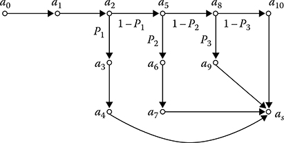
FIGURE 7.7 Flowchart of network graph.

The considered network graph is stochastic without doubt, and there is a need to define the probabilities of transitions between the network graph tops. Let the probability that the selected target pip belongs to the target tracking trajectories be denoted by P₁ = P_tr and processed by the elementary DSP algorithms a₁, a₂, a₃, a₄, a_k. Then,

P' 1 = 1 - P 1 (7.11)

$P_{1}^{'} = 1 - P_{1} (7.11)$

is the probability that the target pip does not belong to the target tracking trajectories and has to be processed further. Let P_D be the probability that the target pip belongs to the detected target track. Then, the probability that the target pip processing is finished by realization of the algorithms a₁, a₂, a₅, a₆, a₇, a_k is defined as

P 2 = (1 - P t r) P D (7.12)

$P_{2} = (1 - P_{t r}) P_{D} (7.12)$

and the probability to proceed with a target pip processing further is determined in the following form:

P' 2 = (1 - P t r) (1 - P D) . (7.13)

$P_{2}^{'} = (1 - P_{t r}) (1 - P_{D}) . (7.13)$

In an analogous way, we obtain

P 3 = (1 - P t r) (1 - P D) P b e g (7.14)

$P_{3} = (1 - P_{t r}) (1 - P_{D}) P_{b e g} (7.14)$

and

P' 3 = (1 - P t r) (1 - P D) (1 - P b e g), (7.15)

$P_{3}^{'} = (1 - P_{t r}) (1 - P_{D}) (1 - P_{b e g}), (7.15)$

where

P_beg is the probability that the target pip belongs to beginning the new target track
P′3 $P_{3}^{'}$ is the probability that the target pip will be assigned as the beginning point of the new target track

The probabilities P_tr, P₀, P_beg depend on the number of target tracking trajectories, detected target tracks, and beginning points of target tracks under processing. For the algorithm of target pip beginning by the criterion (see Chapter 4) we have

The average number of target pips subjected to process under each scanning is determined as

N¯¯¯∑ = N¯¯¯false + N¯¯¯true,(7.16)

where
- N¯¯¯false ${\bar{N}}_{f a l s e}$ is the average number of false target pips
- N¯¯¯true ${\bar{N}}_{t r u e}$ is the average number of true target pips appearing within the limits of the scanning period
The average number of true target pips coming in the target tracking gates under each scanning is given by

$n ¯ s c a n t r u e = P g a t e D N ¯ ¯ ¯ g a t e t r, (7.17)$ ${\bar{n}}_{t r u e}^{s c a n} = P_{D}^{g a t e} {\bar{N}}_{t r}^{g a t e}, (7.17)$

where PgateD $P_{D}^{g a t e}$ is the probability of detection of true target pips within the limits of the target tracking gates, which is the same for all target tracks
The average number of false target pips inside the target tracking gates under each scanning is determined in the following form:

$n ¯ s c a n f a 1 s e = \sum j = m + n m + n + k t h - 1 P s c a n F j N ¯ ¯ ¯ s c a n j, (7.18)$ ${\bar{n}}_{f a 1 s e}^{s c a n} = {\sum^{}}_{j = m + n}^{m + n + k_{t h} - 1} P_{F_{j}}^{s c a n} {\bar{N}}_{j}^{s c a n}, (7.18)$

where

PscanFj $P_{F_{j}}^{s c a n}$ is the probability of the false target pip hit into the jth target tracking gate

N¯¯¯scanj ${\bar{N}}_{j}^{s c a n}$ is the average number of jth target tracking gates for all true and false target tracking trajectories

Taking into consideration (7.16) through (7.18), the probability of an arbitrary selected target pip belonging to one of the target tracking trajectories can be expressed in the following form:

P t r = n ¯ s c a n t r u e + n ¯ s c a n f a 1 s e N ¯ ¯ ¯ Σ . (7.19)

$P_{t r} = \frac{{\bar{n}}_{t r u e}^{s c a n} + {\bar{n}}_{f a 1 s e}^{s c a n}}{{\bar{N}}_{Σ}} . (7.19)$

In an analagous way, we obtain the formula for the probability of target pip belonging to detected target tracks:

P D = n ¯ t r u e D + n ¯ f a l s e D N ¯ ¯ ¯ Σ, (7.20)

$P_{D} = \frac{{\bar{n}}_{D}^{t r u e} + {\bar{n}}_{D}^{f a l s e}}{{\bar{N}}_{Σ}}, (7.20)$

where

n ¯ t r u e D = P D D N ¯ ¯ ¯ t r u e D (7.21)

${\bar{n}}_{D}^{t r u e} = P_{D D} {\bar{N}}_{D}^{t r u e} (7.21)$

and

n ¯ f a l s e D = \sum ​ j = m m + n - 1 P f a 1 s e D j N ¯ ¯ ¯ D j, (7.22)

${\bar{n}}_{D}^{f a l s e} = {\sum^{}}_{j = m}^{m + n - 1} P_{D_{j}}^{f a 1 s e} {\bar{N}}_{D_{j}}, (7.22)$

where

Pfa1seDj $P_{D_{j}}^{f a 1 s e}$ is the probability of the false target pip hit into the detected target track gates with the number j
P_DD is the probability of the true target pip detection into the detected target track gates
N¯¯¯Dj ${\bar{N}}_{D_{j}}$ is the average number of gates with the number j formed by all the detected target tracking trajectories
N¯¯¯trueD ${\bar{N}}_{D}^{t r u e}$ is the average number of the true target tracks being in the detection process

The probability of target pip belonging to the started target tracks is determined as

P b e g = \sum ​ m - n j = 1 P 1 o c k - i n F j N ¯ ¯ ¯ 1 o c k - i n j + P 1 o c k - i n D N ¯ ¯ ¯ 1 o c k - i n t r u e N ¯ ¯ ¯ Σ, (7.23)

$P_{b e g} = \frac{{\sum^{}}_{j = 1}^{m - n} P_{F_{j}}^{1 o c k - i n} {\bar{N}}_{j}^{1 o c k - i n} + P_{D}^{1 o c k - i n} {\bar{N}}_{t r u e}^{1 o c k - i n}}{{\bar{N}}_{Σ}}, (7.23)$

where

Plock−inFj $P_{F_{j}}^{l o c k - i n}$ is the probability of false target pip hit into the primary lock-in gates with the number j
N¯¯¯lock−inj ${\bar{N}}_{j}^{l o c k - i n}$ is the average number of the primary lock-in gates with the number j
Plock−inD $P_{D}^{l o c k - i n}$ is the probability of the true target pip detection into the primary lock-in gates
N¯¯¯lock−intrue ${\bar{N}}_{t r u e}^{l o c k - i n}$ is the average number of the primary lock-in gates of true target tracks

Thus, if the statistical characteristics and parameters of noise and target environment inside the radar coverage are known and the target pip beginning algorithm parameters are selected, in the considered case, we are able to determine the probability of transition in the network graph of the complex DSP algorithm. However, we cannot say that this possibility exists forever. In some cases, the probability of transition can be only estimated as a result of computer simulation of the complex DSP algorithm.

7.3 Evaluation Of Work Content Of Complex Digital Signal Processing Algorithm Realization By Microprocessor Subsystems

7.3.1 EVALUATION OF ELEMENTARY DIGITAL SIGNAL PROCESSING ALGORITHM WORK CONTENT

We consider the DSP algorithms realizing the main operations and control in a CRS as the elementary DSP algorithms:

The signal preprocessing stage: DSP algorithms of matched filtering in time or frequency domains, cancellation of passive interferences by the digital moving target indicator (MTI), detection and estimation of target return signal parameters, recognition of type and estimation of interference and noise parameters and ranking samples, etc
The reprocessing stage: DSP algorithms of target track detection, selection of target pips and their beginning to the target tracking trajectories, target track parameters filtering, transformation coordinate system, and so on
The CRS control process: DSP algorithms of the scanning signal parameter determination under target searching and tracking, determination of power balance between the modes of CRS operations, etc

Each of the aforementioned DSP algorithms is characterized by the work content expressed by the number of arithmetical operations required to realize it. Preliminary computation of the required number of arithmetical operations is possible only if there is an analytical function between the algorithm input and output. In the case of other algorithms possessing a character of logical operations, mainly, the required number of operations can be obtained only as a result of realization based on microprocessor subsystems.

Results of analytical calculation of the required number of arithmetical operations are obtained individually by the number of additions, subtractions, products, and divisions. Henceforth, there is a need to determine the number of reduced arithmetical operations. As the reduction operation, as a rule, an addition is used (short operation). The number of reduced arithmetical operations is determined for each microprocessor subsystem taking into consideration the known ratio between the time to carry out the ith long and short operations, that is, τlongi/τshorti $τ_{i}^{l o n g} / τ_{i}^{s h o r t}$ . However, the computation of the work content is not finished at this stage since we must take into consideration other nonarithmetical operations.

The DSP of target return signals has a pronounced information-logical character. Logical operations and transition operations are for about 80% of the total number of elementary DSP operations (cycles) in the process of the complex DSP algorithm realization required for CRS functioning. For example, under realization of the digital signal preprocessing algorithm of two- coordinate radar system by microprocessor subsystems with permanent memory, the following number of operations in percentage is required: forwarding or transferring—45%; reduced arithmetical operations—23%; control transfer—17%; shift—5%; logical operations—3%; information exchange—2%; other operations—5% Consequently, under computation of the work content of the elementary DSP algorithms there is a need to take into consideration the nonarithmetical operations, too. For this purpose, we can introduce the coefficient K_na and write the following relation:

N ¯ ¯ ¯ j = N ¯ ¯ ¯ a i K n a, K n a > 1, (7.24)

${\bar{N}}_{j} = {\bar{N}}_{a_{i}} K_{n a}, K_{n a} > 1, (7.24)$

where N¯¯¯ai ${\bar{N}}_{a_{i}}$ is the average number of arithmetical operations required for the ith algorithm. The number of microprocessor operations depends on a programming mode. Under the use of high- level programming languages, a program length is two to five times greater than that of the optimal program. To take into consideration this fact, we introduce the coefficient K_prog ≈ 2. Thus, (7.24) can be written in this form:

N ¯ ¯ ¯ j = N ¯ ¯ ¯ a i K n a K p r o g . (7.25)

${\bar{N}}_{j} = {\bar{N}}_{a_{i}} K_{n a} K_{p r o g} . (7.25)$

This work content definition will be used in our next computations.

7.3.2 DEFINITION OF COMPLEX ALGORITHM WORK CONTENT USING NETWORK MODEL

Under analysis of the work content of complex DSP algorithms, we can use the Markov model of computational process or the stochastic network model [3-6]. The stochastic network model allows us to reduce the number of computations under the work content determination in comparison with the Markov model Therefore, we prefer to use the stochastic network model As we noted previously, the network graph model of complex DSP algorithm is the initial condition to evaluate the work content There is a need that this graph would not contain the cycle paths and the graph tops must be numbered in such a way that the graph top number, to which the transition is carried out, will be higher than any graph top number, from which such transition is possible Moreover, the graph end top must have the maximal number k. An example of such graph satisfying all the previously mentioned requirements is depicted in Figure 7.8.

Images

FIGURE 7.8 Example of network graph for complex DSP algorithm.

The average number of addresses to elementary DSP algorithms or the graph tops under a single realization of complex DSP algorithm is denoted by n₁, n₂, ..., n_k−1. Since the graph does not contain the cycles, then at a single realization of the complex DSP algorithm, the average number of hits of the computational process to the graph top with the number i is defined as

n i = \sum ​ j = 0 k - 1 n j P j i, i = 1, 2, ..., k . (7.26)

$n_{i} = {\sum^{}}_{j = 0}^{k - 1} n_{j} P_{j i}, i = 1, 2, ..., k . (7.26)$

Under established order of the top numbering at the instant of computation n_i, the magnitudes of all previous n₁, n₂, ..., n_i-1 are known. The average number of operations under a single realization of the complex DSP algorithm is determined as

M ¯ ¯ ¯ ¯ = \sum ​ i = 1 k n i N ¯ ¯ ¯ j, (7.27)

$\bar{M} = {\sum^{}}_{i = 1}^{k} n_{i} {\bar{N}}_{j}, (7.27)$

where N¯¯¯i ${\bar{N}}_{i}$ is the average number of the elementary DSP algorithm operations corresponding to the ith top of the complex DSP algorithm graph.

Example: There is a need to define the average work content of the complex DSP algorithm presented by the network graph depicted in Figure 7.8 at the following initial conditions: N¯¯¯1=100; N¯¯¯2=30;N¯¯¯3=150;N¯¯¯4=20;N¯¯¯5=200;N¯¯¯6=30 ${\bar{N}}_{1} = 100; {\bar{N}}_{2} = 30; {\bar{N}}_{3} = 150; {\bar{N}}_{4} = 20; {\bar{N}}_{5} = 200; {\bar{N}}_{6} = 30$ P₁₂ = 0.25; P₁₃ = 0.75; P₂₄ = 0.3; P₂₆ = 0.7; P₃₄ = 0.2; P₃₅ = 0.8; P₄₆ = P₅₆ = 1.

Applying (7.26), we obtain

$n 1 = 1, n 2 = n 1 P 12 = 0.25, n 3 = n 1 P 13 = 0.75, n 4 = n 2 P 24 + n 3 P 34 = 0.225, n 5 = n 3 P 35 = 0.6, n 6 = n 2 P 26 + n 46 P 46 = 1. (7.28)$ $n_{1} = 1, n_{2} = n_{1} P_{12} = 0.25, n_{3} = n_{1} P_{13} = 0.75, n_{4} = n_{2} P_{24} + n_{3} P_{34} = 0.225, n_{5} = n_{3} P_{35} = 0.6, n_{6} = n_{2} P_{26} + n_{46} P_{46} = 1. (7.28)$
Applying (7.27), we obtain

$M ¯ ¯ ¯ ¯ = 100 + 30 \times 0.25 + 150 \times 0.75 + 20 \times 0.225 + 200 \times 0.6 + 30 = 374.5. (7.29)$ $\bar{M} = 100 + 30 \times 0.25 + 150 \times 0.75 + 20 \times 0.225 + 200 \times 0.6 + 30 = 374.5. (7.29)$

Thus, the average work content of the complex DSP algorithm presented by the graph depicted in Figure 7.8 is 374.5 reduced arithmetical operations.

If the graph of complex DSP algorithm possesses the cycle paths, we cannot apply the considered procedure to determine the work content M¯¯¯¯ $\bar{M}$ . Owing to this reason, at first, there is a need to exclude the graph cycle paths, that is, to change the graph cycle paths by operator with the equivalent work content The general procedure to transform the graphs of complex DSP algorithms with the purpose of excluding the cycle paths is discussed in Ref. [7]. As an example, we consider a transformation of the graph depicted in Figure 7 9a This graph has several cycles different by rank (the order) The cycles that do not contain in the interior none cycle are covered by the rank 1 The number of iterations for this cycle is denoted by n⁽¹⁾. The cycles consisting of one or several cycles with the rank 1 are covered by the rank 2. The number of iterations for this cycle is denoted by n⁽²⁾, and so on. The graph transform is reduced to changes in cycle paths by a single operator. These changes for the graph shown in Figure 7.9a are carried out in accordance with the following formula:

N 2' = {N ¯ ¯ ¯ 2 + [N ¯ ¯ ¯ 3 + (N ¯ ¯ ¯ 4 + N ¯ ¯ ¯ 5) n (1) + N ¯ ¯ ¯ 6] n (2) + N ¯ ¯ ¯ 7} r (3) . (7.30)

$N_{2}' = {{\bar{N}}_{2} + [{\bar{N}}_{3} + ({\bar{N}}_{4} + {\bar{N}}_{5}) n^{(1)} + {\bar{N}}_{6}] n^{(2)} + {\bar{N}}_{7}} r^{(3)} . (7.30)$

The resulting graph is shown in Figure 7.9b. Thus, the network model of complex DSP algorithm allows us to define, in principle, the average work content. If we know a realization time of a single reduced operation, then we can compute the average realization time of a complex DSP algorithm Inversely, if a limitation on the average realization time of complex DSP algorithm is given, we are able to determine the required work content of microprocessor subsystems to realize the given complex DSP algorithm. Sometimes, to solve the problems of computational resource analysis we need to know information about the work content variance The procedure to define the work content variance is very cumbersome and we do not discuss it in this section.

7.3.3 EVALUATION OF COMPLEX DIGITAL SIGNAL REPROCESSING ALGORITHM WORK CONTENT IN RADAR SYSTEM

We continue consideration and discussion of the example on analysis of the digital signal reprocessing algorithm in CRSs started in Section 7. 1. The initial conditions for analysis are given by the graph flowchart of this algorithm depicted in Figure 7.5. In our analysis, we use the following data:

The average number of tracking targets ${\bar{N}}_{t r}^{g a t e} = 80$
The average number of target tracks under detection ${\bar{N}}_{D}^{t r u e} = 10$
The average number of started target tracks ${\bar{N}}_{b e g} = 5$
The average number of true target pips assigned as the initial points of new target tracks ${\bar{N}}_{i n i t i a l}^{t r u e} = 5$

Thus, the average number of target pips subjected to processing is equal to ${\bar{N}}_{Σ} = 100$ . False target pips and miss of true target pips are not taken into consideration in this example In accordance with the initial conditions, we can compute the following probabilities:

Identification of new target pip among the target tracking trajectories, P_tr = 0.8.
Identification of new target pip among the detected target track, P_D = 0.1.
Identification of new target pip among the begun target tracks, P_beg = 0.05.
The new target pip is assigned as the initial point of new target track, P_new = 0.05

Images

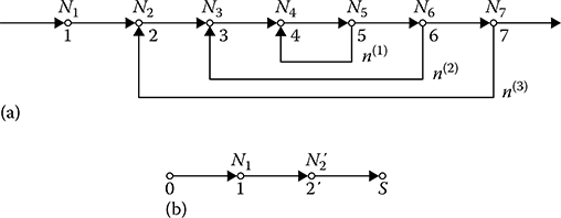
FIGURE 7.9 Example of graph transformation: (a) the graph of cycles different by rank, and (b) the resulting graph.

Images

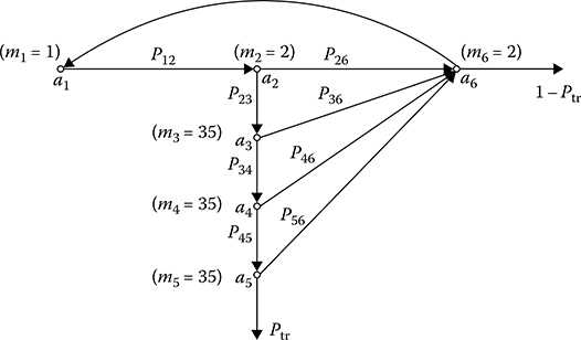
FIGURE 7.10 Typical graph of target and target pip identification algorithm.

Now, we can determine the work content of the elementary DSP algorithms a₁..., a₁₀ including into the complex digital signal reprocessing algorithm presented in Figure 7.7. At first, we consider the typical algorithm of target pip and track identification presented by the graph tops a₂, a₅, a₈. For this purpose, we present this algorithm in the graph form shown in Figure 7.10. The elementary DSP algorithms (operators) are the following:

Selection of the next target pip (or target track parameters) from the corresponding scanned area (the algorithm a₁, Figure 7.10).
Computation $| t_{n} - t_{n - 1} 1 \leq Δ t_{n}^{a c c e p t a b l e}$ (the algorithm a₂, Figure 7.10). A sense of this operation is the following: is it a new or old target track? The work content of this operation is equal to m₂ = 2 of the reduced arithmetical operations.
If the condition 2 is satisfied, a verification of new target pip hit to the gate formed around the extrapolated point of selected target track is carried out This verification is carried out by several stages. At first, the verification is made by the coordinate x(the algorithm a₃), after that by the coordinate y (the algorithm a₄), and finally, by the coordinate z (the algorithm a₅) under the condition that tests using the previous coordinates give us a positive result If at the regular step the conditions are not satisfied, we should follow by the algorithm a₆, that is, to verify the fact that all target tracks of scanned area have been tested. If “No, ” we must carry out a transition to the algorithm aj; if “Yes, ” we should make identification with the next set of target tracks (the output algorithm).

Operations carried out under identification by a single coordinate independently of identified target track kind are the following:

Extrapolation of the selected target track coordinate by the formula

${\hat{x}}_{n}^{e x t r} = {\hat{x}}_{n - 1} + {\hat{\dot{x}}}_{n - 1} Δ t_{n} a n d Δ t_{n} = t_{n} - t_{n - 1} (7.31)$
Computation of the extrapolation error variance by the following formula:

$σ_{{\hat{x}}_{n}^{e x t r}}^{2} = σ_{{\hat{x}}_{n - 1}}^{2} + 2 Δ t_{n} R_{\hat{x} {\hat{\dot{x}}}_{n - 1}} + Δ t_{n}^{2} σ_{{\hat{\dot{x}}}_{n - 1}}^{2}, (7.32)$

where $R_{\hat{x} {\dot{\hat{x}}}_{n - 1}}$ is the correlation function between the target coordinate estimations and velocity at the previous (n − 1)th step.
Computation of the gate dimension by the coordinate

$Δ x_{g a t e} = 3 \sqrt{σ_{{\hat{x}}_{n}^{e x t r}}^{2} + σ_{x m e a s u r e}^{2}} . (7.33)$
Verification of new target pip hit inside the gate

$| x_{_{m e a s u r e}} - {\hat{x}}_{n}^{e x t r} | \leq Δ x_{g a t e} . (7.34)$

Elementary calculations show that under comparison by a single coordinate in accordance with the given formula, there is a need to explore 35 reduced arithmetical operations. Consequently, m₃ = m₄ = m₅ = 35. Under definition of the probabilities Pj in the network graph presented in Figure 7.10, we assume the following:

The number of cancelled target tracks owing to old information does not exceed 1% from the total number of tracking targets. In accordance with this principle, we have P₂₃ = 0.99; P26 = 0.01.
For 95% cases, the identification process is finished after comparison by one coordinate. Because of this, P₃₆ = 0.95; P₃₄ = 0.05.
The probabilities of identification by two and three coordinates are so small that we can neglect these probabilities under determination of the work content of complex DSP algorithm Under computation of the identification algorithm work content, we are able to obtain, individually by each target track array, the following parameters:
1. The minimal work content corresponding to the case when the new target pip is within the limits of the first selected target track gate; the number of reduced arithmetical operations independent of the array equals to
  
  $M_{\min} = m_{1} + m_{2} + m_{3} + m_{4} + m_{5} \approx 100; (7.35)$
2. The maximal work content corresponding to the case when the new target pip is assigned for identification with target tracks of next array after unsuccessful identification with target tracks of the current array; the number of the reduced arithmetical operations for the array of tracking target tracks is given by
  
  $M_{t r}^{\max} = (m_{3} P_{23} + m_{4} P_{34} + m_{5} P_{45}) N_{t r}^{g a t e} \approx m_{3} P_{23} N_{t r}^{g a t e} . (7.36)$

In the case of other arrays, we have

$M_{D}^{\max} \approx m_{3} P_{23} N_{D}^{t r u e}, N_{\max}^{1 o c k - i n} = m_{3} P_{23} N_{t r}^{l o c k - i n} . (7.37)$

The average work content can be determined in the following form:

$\bar{M} = 0.5 (M_{\min} + M_{\max}) . (7.38)$

To simplify further computation, we transform a sequent graph in Figure 7.7 into a parallel graph depicted in Figure 7.11 For this parallel graph, the probabilities of transitions to the graph tops.

Images

FIGURE 7.11 Transformation to parallel graph.

$a_{2}', a_{5}', a_{8}', a_{10}'$ correspond to the probabilities P_tr, P_D, P_beg, P_new, respectively. The average work content for these graph tops is determined in the following form:

${\begin{matrix} M_{2}^{'} & = 0.5 (M_{2}^{\max} + M_{2}^{\min}) = {\bar{M}}_{2}; \\ M_{5}' & = M_{2}^{\max} + 0.5 (M_{5}^{\max} + M_{5}^{\min}) = M_{2}^{\max} + {\bar{M}}_{5}; \\ M_{8}' & = M_{2}^{\max} + M_{5}^{\max} + 0.5 (M_{8}^{\max} + M_{8}^{\min}) = M_{2}^{\max} + M_{5}^{\max} + {\bar{M}}_{8}; \\ M_{10}' & = M_{2}^{\max} + M_{5}^{\max} + M_{8}^{\max} \end{matrix} (7.39)$

Computational results are presented in, Table 7.1.

Now, let us define the work content of other DSP algorithms (the graph tops are depicted in Figure 7.11), taking into consideration the fact that under graph transformation the work content is not changed

The work content of the algorithm aj that is responsible to transform the polar coordinate system to the Cartesian one is directly defined by the coordinate transformation formulas in (5. 149), and recalculation of the correlation matrices of errors of the coordinate measurements depends mainly on a procedure to calculate the trigonometric functions constituent into the coordinate transformation formulas. For example, under representation of sin xand cos x by the limited series expansion, that is,

$\sin x = x - \frac{x^{3}}{3!} + \frac{x^{5}}{5!} + ... a n d \cos x = 1 - \frac{x^{2}}{2!} + \frac{x^{4}}{4!} + ..., (7.40)$

we need 21 additions and 62 multiplications. Taking into consideration that under reducing multiplications to short operations, we use the coefficient of reduction K_red > 1, for our case

TABLE 7.1
Work Content after Transformation of sequent graph to parallel graph

a	$M_{i}^{\max}$	$M_{i}^{m n}$	$M_{i}^{a v}$	$M_{i}'$
$a_{2}'$	100	3200	1650	1650
$a_{5}'$	100	400	250	3450
$a_{8}'$	100	200	150	3750
$a_{10}'$	—	—	—	3800

K_red = 4, to obtain the total number of reduced arithmetical operations characterizing the work content of the algorithm a₁:M₁ ≈ 270.

The work content of the algorithm a₃ is defined by the number of operations required to realize the smoothing filtering algorithm. If the standard recurrent linear filter, for example, Kalman filter, is used for filtering the target tracking trajectory parameters, then for its realization the required number of arithmetical operations is determined by the following formulas:
1. Addition
  
  $n_{a d d} = 2 s^{3} + s^{2} (3 m + h - 1) + s [m (2 m - 1) + (h^{2} - 1)] + m^{2} (m - 1) (7.41)$
2. Multiplication
  
  $n_{m u 1} = 2 s^{3} + s^{2} (3 m + h + 1) + s [2 m (m + 1) + h (h + 1)] + m^{2} (m - 1) (7.42)$
3. Division
  
  $n_{d i v} = m^{2} (7.43)$
  
  where s, m, h are the dimensions of smoothing parameter vectors, measured coordinates, and perturbation actions, respectively. Calculations at s = 6, m = 3, h = 3 gives us the following results n_add = 984, n_mul = 1116, and n_div = 9. After reduction of arithmetical operations, the reduction coefficients $K_{m u l}^{r e d} = 4 a n d K_{d i v}^{r e d} = 7$ , we obtain M₃~ 5500.
4. The work content of the algorithm a₄ is defined by the number of operations required to prepare the user information This process may require a regular or specific transformation of coordinates and target track parameters into the user coordinate system and data extrapolation. In the considered example, we think that M₄ = M₅ ≈ 270.
5. The work content of the algorithm a₅ is defined by the number of operations required to estimate the detected target track parameters based on the fixed sample size. We assume that a target track detection is fixed if the target track beginning defined by two coordinates is confirmed by one more target pip obtained during the next scanning after beginning Consequently, the sample size of observed data under the target track detection is defined by n = 3 In the case of filtering algorithm of polynomial function parameters, the number of operations under the fixed sample size is determined in the following form:
  1. Addition
    
    $n_{a d d} = (s + 1) [(n + s)^{2} + n - 2] + n^{2} (n - 1) (7.44)$
  2. Multiplication
    
    $n_{m u l} = (s + 1) [{(n + s)}^{2} + 3 n + s] + n^{2} (n - 1) (7.45)$
  3. Division
    
    where
    - s is the polynomial order
    - n is the sample size
In the case of linear target track, that is, s = 1 and n = 3, we have M₆ ≈ 400 reduced arithmetical operations.
The work contents of the algorithm a₇ fixing the fact of target track detection and controlling the rerecording of detected target track array to the array of target tracking trajectories, the algorithm a₉ carrying out the estimation of initial magnitudes of initial magnitudes of target track parameters and transferring this estimation to the array of detected target tracks, and the algorithm a₁₀ carrying out a record of target pips as an initial coordinate point of new target tracks can be neglected at this stage owing to simplicity of their realization.

Now, we can determine the average work content of complex DSP algorithm as a whole

$M = M_{1} + P_{t r} (M_{2} + M_{3} + M_{4}) + P_{D} (M_{5} + M_{6} + M_{7}) + P_{b e g} (M_{8} + M_{9}) + P_{n e w} (M_{10} + M_{11}) . (7.47)$

Substituting in (7.47) the values obtained before, we obtain M ≈ 6700. Henceforth, there is a need to take into consideration no arithmetical operations by the corresponding coefficient of reduction $K_{r e d}^{n a}$ . For example, let $K_{r e d}^{n a}$ = 3. Then, we obtain that the total number of operations required for microprocessor subsystem in the case of a single realization of the considered complex digital signal reprocessing can be presented as M ~ 2 x 10⁴ operations. Thus, in the considered example, there is a need to use 2 x 10⁴ microprocessor operations on average to process a single target pip. Naturally, this number corresponds only to the considered algorithm and can be reduced significantly if we are able to upgrade the algorithm of target pip identification, to simplify the algorithm of target track parameters smoothing, etc The main purpose of consideration of this example is to present a possibility to calculate the work content of the complex DSP algorithm and indicate simultaneously some problems arising in the course of these calculations.

7.4 Paralleling Of Computational Process

The results of work content evaluation of the complex DSP algorithm give us the initial information to select the structure and elements of microprocessor subsystems assigned to realize this complex DSP algorithm in a CRS. To ensure the required work content and operational reliability, the designed computational subsystem must include several microprocessor subsystems, as a rule The main peculiarity of these subsystems is instrument or programmable parallelism of the computational process To organize the parallel computational process, there is a need to carry out a paralleling of the complex DSP algorithm. In a general case, the paralleling of the complex DSP algorithms can be considered only for a specific problem taking into consideration the supposed structure of the computational system Consequently, in the course of designing, the problems of selecting a structure of computational system based on the microprocessor subsystems and algorithmic transformation in accordance with the proposed structure of computational system are closely related There is a set of general statements and methods of algorithmic solution paralleling, and we consider some of these methods in this section.

7.4.1 MULTILEVEL GRAPH OF COMPLEX DIGITAL SIGNAL PROCESSING ALGORITHM

The source for paralleling is the graph flowchart of algorithm presented in the multilevel form [8]. The multilevel form is introduced as a generalization of graph flowcharts to illustrate possibilities of serial-parallel operation of algorithms and is a characteristic of the fact that the tops of each level are not related by information features since the final results of operations carried out by one top cannot be considered as initial data for another top. Operations of independent tops (algorithms) can be performed simultaneously Consequently, there is a possibility to realize the elementary DSP algorithms at the definite level using different microprocessor subsystems.

Images

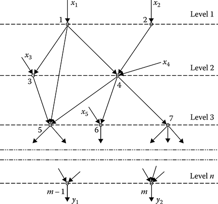
FIGURE 7.12 Multilevel graph of complex DSP algorithm.

The multilevel graph form is obtained in the following way (see Figure 7.12). The first-level top is called the top that has no input arc. The second-level top is the top whose input arc is the output arc of the first-level top. By analogous way, the (n - 1)th level top is the top whose input arc is the output arc of the nth-level top and the output arcs of some previous level tops. In the realization of elementary DSP algorithms, a paralleling is also possible based on the network graph representation of the complex DSP algorithm for the solved problem. In this case, we should transform the initial graph form to the multilevel one In the case of multilevel graph form, each level represents independent elementary DSP algorithms or their set, one of which is carried out necessarily in the course of a single realization of the complex DSP algorithm. If an individual microprocessor subsystem is used to realize the elementary DSP algorithms of each level, we obtain the so-called pipeline subsystem, in which several operations are made simultaneously on data passing in sequence. In this case, the DSP is divided into several stages (by the number of graph levels) and each stage is carried out in parallel with other stages.

To evaluate possibilities of parallel computation organization based on the multilevel algorithmic graph, we introduce a set of quantitative characteristics, namely, b is the ith level width, that i_s, th_e number of independent branches at the ith level; B is the width of the multilevel graph or max{bj; L is the graph length, that is, maximal critical way leading from zero to the final state, i and so on. As follows from the multilevel graph, the realization time of a set of DSP algorithms is limited by some threshold value T_th. By knowing T_th, we can evaluate the required number of the same type of microprocessors N_mp to realize the given set of elementary DSP algorithms. In doing so, we obtain

$N_{m p} \leq \frac{T_{m p}^{s i n g l e}}{T_{t h}}, (7.48)$

where

$T_{m p}^{s i n g l e} = {\sum^{}}_{i = 1}^{m} t_{i}$ is the realization time of all algorithms for a single microprocessor subsystem
t_t is the realization time of the ith elementary DSP algorithm
m is the number of elementary DSP algorithms in the complex one

We consider a design procedure of the multilevel graph using an example of algorithm paralleling for the linear recurrent filtering of target track parameters given by the state equation (5.1). In the given case, the linear recurrent filtering algorithm takes the following form:

${\begin{matrix} {\hat{θ}}_{e x_{n}} & = Φ_{n} θ_{n - 1} + Γ_{n} η_{n - 1}; \\ Ψ_{e x_{n}} & = Φ_{n} Ψ_{n - 1} Φ_{n}^{T} + Γ_{n} Ψ_{η} Γ_{n}^{T}; \\ G_{n} & = Ψ_{e x_{n}} H_{n}^{T} {(H_{n} Ψ_{e x_{n}} H_{n}^{T} + R_{n})}^{- 1}; \\ {\hat{Y}}_{e x_{n}} & = H_{n} {\hat{θ}}_{e x_{n}}; \\ {\hat{θ}}_{n} & = {\hat{θ}}_{e x_{n}} + G_{n} (Y_{n} - {\hat{Y}}_{e x_{n}}); \\ Ψ_{n} & = Ψ_{e x_{n}} - G_{n} H_{n} Ψ_{e x_{n}}, \end{matrix} (7.49)$

where

θ_n is the (s × 1) vector of estimated target track parameters
θ_{ex_n} is the (s × 1) vector of extrapolated target track parameters
Y_n is the (m × 1) vector of measured coordinate magnitudes
Y_{ex_n} is the (m × 1) vector of extrapolated coordinate magnitudes
η_n−1 is the (h × 1) vector of disturbance of target track parameters
Φ_n is the transfer (s × s) matrix of target track model
Ψ_n is the correlation (s × s) matrix of errors of target track parameter estimation
Ψ_{ex_n} is the correlation (s × s) matrix of extrapolation of target track parameters
Ψ_η is the correlation (h × h) matrix of target track random disturbances
Γ_n is the (s × h) matrix (see (5. 1))
H_n is the (m × s) matrix (see (5. 11))
R_n is the correlation (m × m) error matrix of target track coordinate measurements

Dimensions of matrices and vectors are required in determination of the work content for the branches of the multilevel complex DSP algorithm graph.

The ordinary complex DSP algorithm graph is the basis for the multilevel graph. In the case of ordinary complex DSP algorithm graph, the two-input functional operators on vector and matrices are considered as the tops and results of operations, and transitions in the graph are considered as the arcs In doing so, a set of arcs without initial tops is an ensemble of initial arguments, and a totality of arcs without the end tops is a set of output results The graph, as a rule, is designed manually because to formalize this process is a very difficult problem. The initial graph of linear filtering algorithm is depicted in Figure 7.13. To design the multilevel graph, at first, we should present the initial graph in the form of adjacency matrix with the number of columns and rows equal to the number of initial graph tops. The elements of the adjacency matrix lj take the value 0 if there is no arc between the top i and the top j and the value 1 if there is an arc between the top i and the top j. The adjacency matrix elements of the multilevel graph shown in Figure 7.13 are represented in Table 7.2.

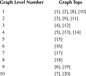
The transformation process of the initial complex DSP algorithm graph into the multilevel complex DSP algorithm graph is to sort the adjacency matrix rows and columns and is based on an adjacency matrix feature to have zero rows if there are end tops and zero columns if there are initial tops, that is, all arcs for these tops are initial. In our case, the tops “1,” “2,” “8,” and “10” are the initial tops. These tops form the first level of the sorted multilevel graph. The next step is nulling all the nonzero elements of rows with the numbers selected at the first step. At the same time, the first level tops are considered as the end tops and the output arcs are considered as the input arcs for the higher level (next level). Henceforth, we search for columns not marked previously of the adjacency matrix with zero elements. The numbers of these columns form the second-level tops and so on until all columns will be numbered. As a result, we obtain the table with the numbers of levels and graph tops corresponding to each level. For the considered case, a distribution of tops along the levels is presented in Table 7.3. Using Table 7.3 and taking into consideration relations between the initial graph tops presented in Figure 7.14, the multilevel complex DSP algorithm of linear filtering has been designed. There is a need to note that the multilevel graph form depends on a sequence based on how this graph is designed, namely, starting from a set of tops as in designing the graph depicted in Figure 7.14 or starting from a set of output tops. In the last case, a distribution of tops by levels is presented in Table 7.4 and the corresponding multilevel graph is depicted in Figure 7.15. As we can see, in this case, the graph is different from the previous one.

Images

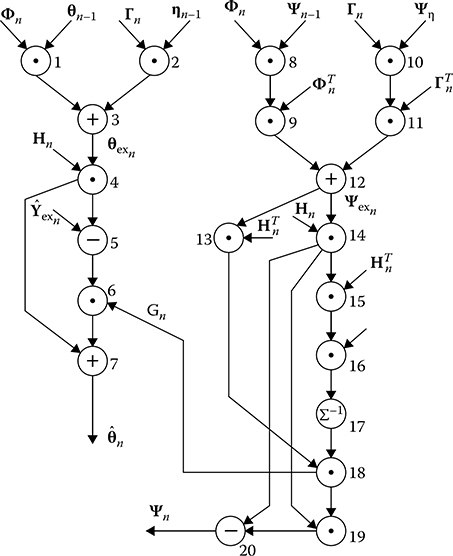
FIGURE 7.13 The multilevel graph of linear filtering algorithm.

TABLE 7.2
Adjacency Matrix Elements of the Multilevel Graph Shown in Figure 7.13

Images

TABLE 7.3
Distribution of Graph Tops along the Levels

Images

A simple consideration of multilevel graph indicates that there is a possibility to parallel a computational process under realization of the corresponding complex DSP algorithms. As follows from Figures 7.14 and 7.15, more than one macro-operations (from 1 to 3) can be carried out simultaneously under realization of the linear filtering algorithm. Consequently, several microprocessor subsystems, namely, from 1 to 3, respectively, can participate in the computational process. In doing so, the realization time of the complex DSP algorithm can be reduced essentially, since instead of 20 macro-operations carried out in sequence by one microprocessor subsystem there is a need to carry out not more than 10 macro-operations for each microprocessor subsystem in parallel scheme.

Images

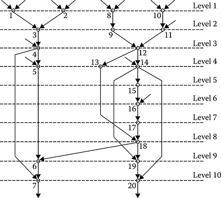
FIGURE 7.14 Tops of initial graph.

TABLE 7.4
Distribution of Graph Tops along the Levels

Images

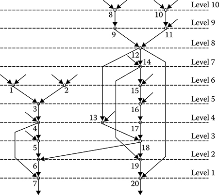
FIGURE 7.15 Multilevel graph.

Further transformations of the multilevel graphs can be carried out in two avenues: (a) definition of rational number of microprocessor subsystems realizing the paralleling complex DSP algorithm within the limits of the given minimal time and (b) optimal distribution of macro-operations by microprocessor subsystems if the number of microprocessor subsystems is given and their characteristics are known and the minimal realization time is a criterion of effectiveness. To solve both the first and the second problems, there is a need to obtain additional information concerning the weights of graph tops, that is, the number of elementary operations carried out during a realization of all macro-operations, by which the graph tops are marked.

7.4.2 PARALLELING OF LINEAR RECURRENT FILTERING ALGORITHM MACRO-OPERATIONS

Consider the computational process paralleling problem for the given number, in our case two, of the same type of microprocessor systems based on the example of the linear recurrent filtering algorithm. To solve this problem, first, there is a need to compute the work content of the multilevel graph tops of the considered linear recurrent filtering algorithm. The graph depicted in Figure 7.15 is considered as the basis. Number the tops of this graph from right to left and top-down and define the macro-operations carried out under transition to each top. As noted earlier, these macrooperations are the two-input operations on the vectors and matrices and one operation of the matrix inversion Table 7.5 represents the operations corresponding to the graph tops and expressions to compute the number of arithmetical operations under realization of corresponding operators by the microprocessor systems The number of reduced arithmetical operations for each graph operator is determined at s = 6, m = 3, h = 3. The arithmetical operation reduction, as earlier, is carried out taking into consideration the fact that the multiplication operation can be accomplished by the microprocessor system in four cycles and the division operation—for seven cycles. Next columns of Table 7.5 present the results of the work content computation for the graph tops taking into consideration nonarithmetical operations. The multilevel graph tops shown in Figure 7.16 are marked by these computational results.

TABLE 7.5
Operations Corresponding to the Graph Tops and Expressions to Compute the Number of Arithmetical Operations

Images

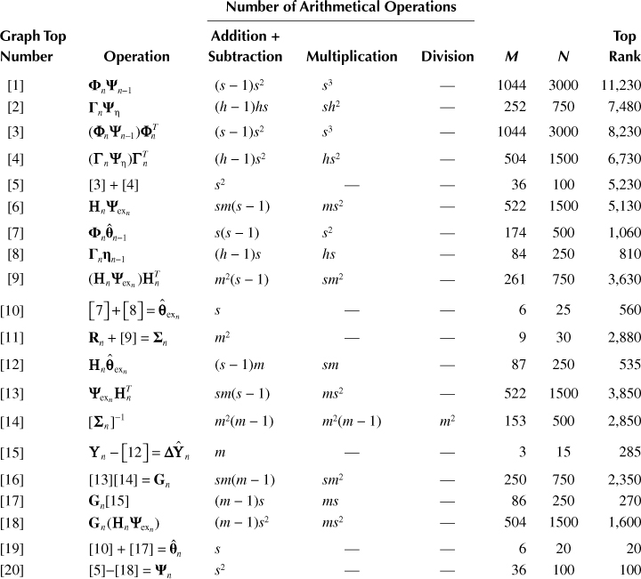
FIGURE 7.16 Multilevel graph.

Now, let us start a direct distribution of the graph tops by microprocessor subsystems. The distribution is carried out in the following sequence:

The graph top ranking is carried out—the weight equal to maximal way (by the operation number) leading from the given top to the end top (the top ranks are given in the last column of Table 7.5 and designated by the numbers in parentheses in Figure 7.16) is assigned to each graph top.
The graph top with the maximal rank (the top 1) is assigned for the first microprocessor subsystem The graph top with the maximal rank after loading the first microprocessor subsystem and not requiring results of operations made by the first microprocessor subsystem is assigned for the second microprocessor subsystem (the top 2)
The remaining graph tops with maximal rank are assigned to realize the given algorithm under the condition that there are required data. If the required data are not available or absent, a microprocessor subsystem is in the standby mode until obtaining the required data from other microprocessor subsystem

$K_{l o a d} = \frac{M_{t o t a l}}{2 N_{t h}} 0.725. (7.50)$

Thus, we cannot say that a paralleling of the considered algorithm by this way is an ideal process with the viewpoint of loading the two microprocessor subsystems To increase the coefficient of loading K_load of microprocessor subsystems, there is a need to decrease a length of macro-operations and to carry out paralleling computations inside each macro-operation.

Images

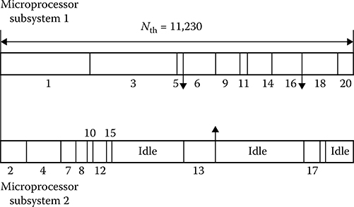
FIGURE 7.17 Loading schedules of microprocessor subsystems.

In conclusion, we note that the considered example is purely illustrative. We do not take into consideration any possibility of reducing the number of operations under realization of some graph tops, for example, owing to matrix set sparseness including in the algorithmic formula flowchart, special procedures in carrying out the specific vector-matrix operations, and so on. The reduction coefficients of multiplication and division operations to short operations are conditional, etc.

7.4.3 PARALLELING PRINCIPLES OF COMPLEX DIGITAL SIGNAL PROCESSING ALGORITHM BY OBJECT SET

Under complex DSP, we consider a set of objects, namely, the target return signals, target pips, target tracks, and so on Information about these objects must be processed using the same complex DSP algorithms If the considered objects are independent, then information about each object can be processed independently. In this case, we use the independent objects paralleling. Consider some examples when we use the paralleling principles for independent objects at different levels of complex DSP algorithm for the surveillance radar.

Example 1: Consider the multichannel receiver with signal preprocessing assigned to detect the targets and estimate the target pip parameters under the radar coverage scanning (see Figure 7.18). The receiver consists of the multichannel microprocessor subsystem representing a set of specific signal processing processors and the general controlling processor carrying out the functions of new information distribution by channels We assume that the number of parallel signal processing channels is equal to or less than the number of independent target return signal sources. As the independent target return signal sources, we consider, in this case, the intervals of incoming stochastic process within the limits of each discrete time interval In doing so, we suppose that a time discretization frequency of the input stochastic process is selected in such a way that the signals from the neighbor discrete time intervals are statistically independent The signals are accumulated, the target pips are formed, the signal detection problems are solved, the target pip coordinates are defined, and the target pip coordinates are transferred to the user by each channel of the multichannel receiver. The period of incoming new signal to each channel of the multichannel receiver corresponds to the period of scanning signals sending. Because of this, the requirements to parameters of processors possess medium character. Another advantage of the considered multichannel receiver is low power consumption to distribute the problems by channels.

Images

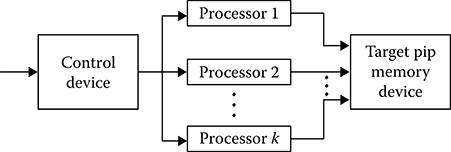
FIGURE 7.18 Multichannel receiver with digital signal reprocessing algorithm.

Images

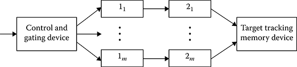
FIGURE 7.19 Target autotracking system flowchart.

Example 2: Consider an organization of target trajectory autotracking by the autonomous microprocessor subsystems carrying out a whole cycle of signal processing by a single target This target tracking system (see Figure 7.19) consists of m channels (microprocessor subsystems). The signal detection algorithms, the definition and measurement of signal parameters, and the signal selection in the physical gates of individual target tracking (block 1), the algorithm of estimation of target track parameters, and sending the final information to the system forming a general location situation (block 2) are realized by each channel of the target autotracking system. In a general case, each of the complex DSP algorithms (signal preprocessing and signal reprocessing) can be realized by individual specific microprocessor subsystems In this case, the number of signal preprocessing and signal reprocessing channels can be considered different Additionally, the target autotracking system contains the microprocessor subsystems realizing the control and commutation of signal processing channels and gating the receivers This target autotracking system allows us to organize the complex signal processing algorithm for target return signal in real time by microprocessor subsystems with limited productivity.

Example 3: Consider an organization of paralleling under the DSP of target return signals from Mindependent CRSs using a computer system based on N microprocessor subsystems. The DSP algorithm is to define the target tracks by the target pips sent by each radar system or signal preprocessing subsystem All radar systems operate in asynchronous mode, and their radar coverage of each radar system is overlapped with other ones The computer system under the parallel DSP depicted in Figure 7.20 contains an associative addressing device in addition to microprocessor subsystems, which allows us to carry out simultaneously a comparison of each target pip coordinate coming from radar systems jointly with the gates of extrapolated points of all target trajectories tracked by radar systems simultaneously. On-stream of the computer system, each microprocessor subsystem sends to the associative addressing device the gates of such targets that are processed by the microprocessor subsystem at the current time. All the gates are extrapolated with a definite cycle in such a way that the incoming new target pips and extrapolated points of target tracks are obtained at the same time. Information about the target pips comes in at the associative addressing device input from the CRS output, and the associative addressing device defines which microprocessor subsystem must process the incoming target pip based on an associative comparison of boundaries of all the gates. The target pip is sent to the corresponding microprocessor subsystem to renew information about the specific target If the target pip belongs to a new target, that is, there is no gate to which this target pip can belong, then the information goes to one from the microprocessor subsystem that is not loaded completely. We can control the loading process of the microprocessor subsystems. For this purpose, there is a need to determine the coefficients of current loading of all the microprocessor subsystems for each scanning cycle T_scan:

Images

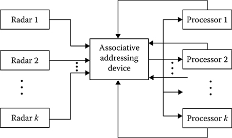
FIGURE 7.20 Computer system with DSP algorithm paralleling.

$K_{i j}^{l o a d} = \frac{T_{i j}}{T_{s c a n}}, (7.51)$

where

T_ij is the time required for the ith microprocessor subsystem under the jth scanning to process all targets
T_scan is the scanning cycle

To increase the control stability, we define the averaged by n scans coefficient of loading in the following form:

$K_{i}^{l o a d} = \frac{1}{n} {\sum^{}}_{j = 1}^{n} K_{i j}^{l o a d} . (7.52)$

The loading coefficient is defined more exactly after each scanning. If all $K_{i}^{l o a d}$ = 1, i = 1,..., N, then the microprocessor subsystem and, consequently, the computer system have been loaded completely and under upcoming new target pip belonging to the new target tracks, the computer system is overloaded and, consequently, the microprocessor subsystems are overloaded, too, and the corresponding control signal informs us about this situation The computer system consisting of the microprocessor subsystems can be designed in such a way that, at first, the first microprocessor system is overloaded, after that the second microprocessor subsystem is overloaded, and so on. Under this type of computer system organization, it is simpler to take into consideration an incomplete microprocessor subsystem capacity and organize the complete capacity.

The discussed paralleling computer system consisting of the microprocessor subsystems and carrying out the digital signal reprocessing algorithms has a high reliability and operability and, additionally, ensures high-quality user information about the tracking targets The disadvantage of this complex digital signal reprocessing algorithm paralleling is a necessity to use a very complex associative addressing device, especially, if the number of tracking targets is high.

7.5 Summary And Discussion

The exponential growth in digital technology since the 1980s, along with the corresponding decrease in its cost, has had a profound impact on the way radar systems are designed. More and more functions that were historically implemented in analog hardware are now being performed digitally, resulting in increased performance and flexibility and reduced size and cost. Advances in ADC and DAC technologies are pushing the border between analog and digital processing closer and closer to the antenna. In the past, implementing a real-time radar digital signal processor typically required the design of a custom computing machine, using thousands of high-performance ICs. These machines were very difficult to design, develop, and modify. Digital technology has advanced to the point where several implementation alternatives exist that make the processor more programmable, and easier to design and change.

The parallel microprocessor subsystem architecture employs multiple general-purpose processors that are connected via high-speed communication networks Included in this class are high-end servers and embedded processor architectures. Servers are typically homogeneous processors, where all of the processing nodes are identical and are connected by a very high- performance data bus architecture Embedded processor architectures are typically composed of single-board computers (blades) that contain multiple general-purpose processors and plug into standard backplane architecture This configuration offers the flexibility of supporting a heterogeneous architecture, where a variety of different processing blades or interface boards can be plugged into the standard backplane to configure a total system It is apparent that high-speed serial links will be the primary communication mechanism for multiprocessor subsystems into the future, with ever-increasing data bandwidths These parallel microprocessor subsystem architectures offer the benefit of being programmable using high-level languages, such as C and C++. A related advantage is that programmers can design the system without knowing the intimate details of the hardware. In addition, the software developed to implement the system can typically be moved relatively easily to new hardware architecture as part of a technology refresh cycle. On the negative side, these systems can be difficult to program to support real-time signal processing. The required operations need to be split up appropriately among the available processors, and the results need to be properly merged to form the final result. A major challenge in these applications is to support the processing latency requirements of the system, which defines the maximum length of time allowed to produce a result. The latency of the microprocessor subsystem is defined as the amount of time required to observe the effect of a change at a processor’s input on its output Achieving latency goals often requires assigning smaller pieces of the workload to individual processors, leading to more processors and a more expensive system Another challenge facing these systems in radar application is reset time In a military application, when a system needs to be reset in order to fix a problem, the system needs to come back to full operation in a very short period of time These microprocessor subsystems typically take a long time to reboot from a central program store and, hence, have difficulty meeting reset requirements Developing techniques to address these deficiencies is an active area of research. Finally, these processors are generally used for non-real time or near-real-time data processing, as in target tracking and display processing. Since the 1990s, they have started to be applied to real-time signal processing applications Although they might be cost-effective for relatively narrowband systems, their use in wideband DSP systems in the early twenty-first century is typically prohibitively expensive due to the large number of processors required This situation should improve over time as faster and faster processors become available.

The introduction of the FPGA in the 1980s heralded a revolution in the way real-time DSP systems were designed. FPGAs are integrated circuits that consist of a large array of configurable logic elements that are connected by a programmable interconnect structure At the time of this writing, FPGAs can also incorporate hundreds of multipliers that can be clocked at rates up to a half billion operations per second, and memory blocks, microprocessors, and serial communication links that can support multigigabit-per-second data transfers FPGAs allow the designer to fabricate complex signal processing architectures very efficiently In typical large applications, FPGA-based processors can be a factor of 10 (or more) smaller and less costly than systems based on general-purpose processors This is due to the fact that most microprocessors only have one or very few processing elements, whereas FPGA have an enormous number of programmable logic elements and multipliers. On the negative side, utilizing an FPGA to its best advantage typically requires the designer to have a thorough understanding of the resources available in the device. This typically makes efficient FPGA-based systems harder to design than radar systems based on general-purpose processors, where a detailed understanding of the microprocessor subsystem architecture is not necessarily required. In addition, FPGA designs tend to be aimed at a particular family of devices and take full advantage of the resources provided by that family. Hardware vendors are constantly introducing new products, invariably incorporating new and improved capabilities. Over time, the older devices become obsolete and need to be replaced during a technology refresh cycle. When a technology refresh occurs several years down the road, typically the available resources in the latest FPGAs have changed or a totally different device family is used, which probably requires a redesign On the other hand, software developed for general-purpose processors may only need to be recompiled in order to move it to a new processor Tools currently exist that synthesize C or MATLAB code into a FPGA design, but these tools are typically not very efficient The evolution of design tools for FPGAs to address these problems is an area of much research and development.

The complex algorithm of the computational process is a set of elementary DSP algorithms for all stages and CRS modes of operation. Off-line complex algorithms of individual stages of DSP, which are not associated with one another by information processes and control operations, are possible, too To design the complex algorithm of the computational process, there is a need to have an unambiguous definition of microprocessor subsystem functioning in the solution of goal-oriented DSP problems This definition must include the elementary DSP and control algorithms, a sequence of their application, the conditions of implementation of each elementary DSP and control algorithm, and intercommunication between the DSP and control algorithms using input and output information A general form of such definition and description can be presented using the logical and graph flowchart of the DSP and control algorithms.

One of the best-known ways to assign the complex algorithm in depending on complexity is the logical or formula-logical algorithmic flowchart. The elementary operators and recognizers are presented in a geometrical form in the logical algorithm flowchart (rectangle, jewel boxes, trapeziums, etc.) connected with each other by arrows in accordance with the given sequence order of counting operators and recognizers in the complex algorithm Titles of elementary operations (DSP algorithms) are written inside the geometrical forms Sometimes the formulas of logical operations carried out and logical conditions under test are written inside the geometrical forms In this case, the corresponding logical flowchart of the algorithm is called the formula-logical block diagram.

The main problems solved by the graph flowcharts of complex algorithms are a definition of rational ways to present these problems and a choice of computational software tools and microprocessor subsystems to realize the complex DSP algorithm of a radar system In short, the problem of optimization of computational process is assigned The solution of this problem allows us to reduce significantly the realization time and to simplify the complex DSP algorithm of the radar system Similar problems are the problems of network planning and control.

The deterministic network model cannot present a complex DSP algorithm functioning in a CRS since it is impossible to predict a set of elementary DSP algorithms and sequence of realizations for each practical situation Therefore, the stochastic network model, in which the transitions in the network graph are defined by the corresponding probabilities of transitions given by specific conditions of CRS functioning, is more suitable to image and analyze a realization of complex algorithm by microprocessor systems When the network model has been constructed, the problem to estimate the time to complete all operations, that is, the time to finish all operations by microprocessor subsystems with the given effective speed of operations, arises This time cannot be higher than a total duration to finish a complex algorithm operation defined in the most unfavorable way from the initial graph top a_n to the final graph top a_k, that is, along such a route that generates a maximal duration of operations. This route is called extreme. The extreme route in the stochastic network model cannot be presented in clear form as, for example, in the network model with a given structure. Because of this, the problems of defining the average time or average number of operations required to realize the complex algorithm are assigned under analysis of stochastic network models. If the statistical characteristics and parameters of noise and target environment inside the radar coverage are known and the target pip beginning algorithm parameters are selected, we are able to determine the probability of transition in the network graph of the complex DSP algorithm. However, we cannot say that this possibility exists forever. In some case, the probability of transition can only be estimated as a result of computer simulation of the complex DSP algorithm.

Results of analytical calculation of the required number of arithmetical operations are obtained separately by the number of additions and subtractions, products, and divisions There is a need to determine the number of reduced arithmetical operations. As the reduction operation, as a rule, an addition is used (short operation). The number of reduced arithmetical operations is determined for each microprocessor subsystem taking into consideration the known ratio between the time to carry out the ith long and short operations. The DSP of target return signals has a pronounced information-logical character. Logical operations and transition operations are for about 80% of the total number of elementary DSP operations (cycles) in the process of realization of the complex DSP algorithm required for CRS functioning. Consequently, under the work content computation of the elementary DSP algorithms there is a need to take into consideration the nonarithmetical operations, too. Under the work content definition, we must take into consideration additionally that the number of microprocessor operations depends on a mode of programming.

The network model of complex DSP algorithm allows us to define, in principle, the average work content If we know the realization time of a single reduced operation, then we can compute the average realization time of a complex DSP algorithm Inversely, if a limitation on the average realization time of a complex DSP algorithm is given, we are able to determine the required work content of microprocessor subsystems to realize the given complex DSP algorithm Sometimes, to solve the problems of computational resource analysis we need to know information about the work content variance.

Henceforth, there is a need to take into consideration the nonarithmetical operations by the corresponding coefficient of reduction $K_{r e d}^{n a}$ . For example, let $K_{r e d}^{n a}$ = 3; then we obtain that the total number of operations required for a microprocessor subsystem in the case of a single realization of the considered complex digital signal reprocessing can be presented as M ≈ 2 x 10⁴ operations. Thus, in the considered example, there is a need to use 2 x 10⁴ microprocessor operations on average to process a single target pip. Naturally, this number corresponds only to the considered algorithm and can be reduced significantly if we are able to upgrade the algorithm of target pip identification, to simplify the algorithm of target track parameters smoothing, etc The main purpose of consideration of this example is to present a possibility of calculating the work content of the complex DSP algorithm and indicate simultaneously some problems arising in the course of these calculations.

The results of work content evaluation of the complex DSP algorithm give us the initial information to select the structure and elements of microprocessor subsystems assigned to realize this complex DSP algorithm in a CRS. To ensure the required work content and operational reliability, the designed computational system must include several microprocessor subsystems, as a rule The main peculiarity of these microprocessor subsystems is instrument or programmable parallelism of computational process To organize the parallel computational process, there is a need to carry out a paralleling of the complex DSP algorithm. In a general case, the paralleling of complex DSP algorithms can be considered only for a specific problem taking into consideration the supposed structure of a computational subsystem Consequently, in the course of designing, the problems of selecting the structure of a computational subsystem based on the microprocessor subsystems and algorithmic transformation in accordance with the proposed structure of the computational subsystem are closely related. There is a set of general statements and methods of algorithmic solution paralleling.

A simple consideration of the multilevel graph indicates that there is a possibility to parallel a computational process under realization of the corresponding complex DSP algorithms. As follows from Figures 7.14 and 7.15, more than one macro-operations (from 1 to 3) can be carried out simultaneously in the realization of the linear filtering algorithm. Consequently, several microprocessor subsystems, namely, from 1 to 3, respectively, can participate in the computational process. In doing so, the realization time of the complex DSP algorithm can be reduced essentially, since instead of 20 macro-operations carried out in sequence by one microprocessor system there is a need to carry out not more 10 macro-operations for each microprocessor subsystem in parallel scheme.

Further transformations of the multilevel graphs can be carried out in two avenues:

Definition of a rational number of microprocessor subsystems realizing the paralleling complex DSP algorithm within the limits of the given minimal time.
Optimal distribution of macro-operations by microprocessor subsystems if the number of microprocessor subsystems is given and their characteristics are known and the minimal realization time is a criterion of effectiveness.

To solve both the first and the second problems, there is a need to obtain additional information concerning the weights of graph tops, that is, the number of elementary operations carried out during the realization of all macro-operations, by which the graph tops are marked.

The loading schedule of microprocessor subsystems is presented in Figure 7.17. As follows from Figure 7.17, the threshold number of microprocessor subsystem operations under paralleling on two microprocessor subsystems is defined as N_th = 11,230 operations under the condition that the total work content of the considered algorithm is given by M_total = 16,290 operations. The second microprocessor subsystem is loaded only on 45%. The coefficient of microprocessor subsystem loading K_load can be defined by (7.50). Thus, we cannot say that a paralleling of the considered algorithm by this way is an ideal process with the viewpoint of loading the two microprocessor subsystems To increase the coefficient of loading K_load of microprocessor subsystems, there is a need to decrease a length of macro-operations and to carry out paralleling computations inside each macro-operation.

Under complex DSP, we consider a set of objects, namely, the target return signals, target pips, target tracks, and so on Information about these objects must be processed using the same complex DSP algorithms If the considered objects are independent, then information about each object can be processed independently In this case, we use the independent objects paralleling.

The discussed paralleling computer system consisting of the microprocessor subsystems and carrying out the digital signal reprocessing algorithms has a high reliability and operability and, additionally, ensures high-quality user information about the tracking targets The disadvantage of this complex digital signal reprocessing algorithm paralleling is the necessity to use a very complex associative addressing device, especially if the number of tracking targets is high.

References

1. Rahnema, M. 2007. UMTS Network Planning, Optimization, and Interoperation with GSM. New York: John Willey & Sons, Inc.

2. Laiho, J., Wacker, A., and T. Novosad. 2006. Radio Network Planning and Optimization for UMTS. 2nd Edn. New York: John Wiley & Sons, Inc.

3. Woolery, J. and K. Crandall. 1983. Stochastic network model for planning scheduling. Journal of Construction Engineering and Management, 109(3): 342–354.

4. Butler, R. and A. Huzurbazar. 1997. Stochastic network models for survival analysis. Journal of the American Statistical Association, 92(437): 246–257.

5. Tsitsiashvili, G. and M. Osipova. 2008. Distributions in Stochastic Network Models. New York: Nova Publishers.

6. Neely, M. 2010. Stochastic Network Optimization with Application to Communication and Queuing Systems. Synthesis Lectures on Communication Networks. Los Angeles, CA: Morgan & Claypool Publishers

7. Creebery, D. and D. Golenko-Ginzburg. 2010. Upon scheduling and controlling large-scale stochastic network project. Journal of Applied Quantitative Methods, 5(3): 382–388.

8. Pospelov, D. 1982. Introduction to Theory of Computational Systems. Moscow, Russia: Soviet Radio (in Russian)

..................Content has been hidden....................

You can't read the all page of ebook, please click here login for view all page.

Table of Contents for Chapter 7 Design Principles of Complex Algorithm Computational Process in Radar Systems

Create new playlist

Sign In

Sign Up

Table of Contents for
Chapter 7 Design Principles of Complex Algorithm Computational Process in Radar Systems