11.1 Main Definitions and Problem Statement

In a general form, the problem of estimates of stochastic process parameters can be formulated in the following manner. Let the incoming realization x(t) or a set of realizations x_i(t), i = 1,…, ν of the random process ξ(t) be observed within the limits of the fixed time interval [0, T]. In general, the multidimensional (one-dimensional or n-dimensional) probability density function (pdf) of the random process ξ(t) contains μ unknown parameters l = {l₁, l₂, …, l} to be estimated. We assume that the estimated multidimensional parameter vector l = {l₁, l₂, …, l} is the continuous function within the limits of some range of possible values ℒ. Based on observation and analysis of the incoming realization x(t) or realizations x_i(t), i = 1,…, ν, we need to decide what magnitudes from the given domain of possible values possessing the parameters l = {l₁, l₂, …, l_μ} are of interest for the user. Furthermore, only the realization x(t) of the random process ξ(t) is considered if the special conditions are not discussed. In other words, we need to define the estimate of the required multidimensional parameter l = {l₁, l₂, …, l_μ} on processing the observed realization x(t) within the limits of the fixed time interval [0, T].

Estimate of the parameter l = {l₁, l₂,…, l} of the random process ξ(t) is a set of functions or a single function of the observed data x(t). The values of these functions for the fixed realization x(t) estimate, that is, defined by a given way, are the unknown parameters of stochastic process. Depending on the requirements of estimation process and estimates of parameters, various estimation procedures are possible. In doing so, each estimate is characterized by its own quality performance that, in majority of cases, indicates a measure of the estimate’s closeness to the true value of estimated random process parameter. The quality performance, in turn, is defined by a choice of estimation criterion. Because of this, before estimate definition, we need to define a criterion of estimation. Selection of estimate criterion depends on the end problem, for which this random process parameter estimate is used. Because these problems can differ substantially, it is impossible to define and use the integrated criterion and one common estimate for the given random process parameter. This circumstance makes it difficult to compare various estimates.

In many practical applications, the estimate criteria are selected based on assumption about the purpose of estimate. At the same time, a design of process to choose definite estimate criteria is of great interest because such approach allows us to understand more clearly the essence and characteristic property of the problem to estimate the random process parameter and, that is very important, gives us a possibility to define the problem of valid selection of the estimate criterion more fairly. Owing to the finite time of observation and presence of noise and interference concurrent to observation, specific errors in the course of estimate definition arise. These errors are defined both by the quality performance and by conditions under which an estimation process is carried out. Because of this, the problem of optimal estimation of the parameter l = {l₁, l₂,…,l_μ} is to define a procedure that allows minimizing the errors in estimation of the parameter l = {l₁, l₂,…,l_μ}. In general, the requirement of minimizing estimation error is not based on one particular aspect. However, if the criterion of estimation is given, the quality performance is measured using that criterion. Then the problem of obtaining the optimal estimation is reduced to a definition of solution procedure that minimizes or maximizes the quality performance. In doing so, the parameter estimate must be close, in a certain sense, to the true value of estimated parameter, and the optimal estimate must minimize this measure of closeness in accordance with the chosen criterion.

To simplify the written form and discussion in future, we assume, if it is not particularly fixed, that the unknown parameter of the random process ξ(t) is the only parameter l = {l₁, l₂,…, l_μ}. Nevertheless, all conclusions made based on our analysis of estimation process of the parameter l = {l₁, l₂,…, l_μ} of the random process ξ(t) are correct with respect to joint estimation process of several parameters of the same random process ξ(t). Thus, it is natural to obtain one function from the observed realization x(t) to estimate a single parameter l = {l₁, l₂,…, l_μ} of the random process ξ(t). Evidently, the more knowledge we have about the characteristics of the analyzed random process ξ(t) and noise and interference in the received realization x(t), the more accurate will be our estimation of possible values of the parameters of the random process ξ(t), and thus more accurate will be the solution based on synthesis of the devices designed using the chosen criterion with the minimal errors in the estimation of random process parameters of interest.

More specifically, the estimated parameter is a random variable. Under this condition, the most complete data about the possible values of the parameter l = {l₁, l₂,…, l_μ} of the random process ξ(t) are given by the a posteriori pdf p_post(l) = p{l|x(t)}, which is the conditional pdf if the given realization x(t) is received. The formula of a posteriori pdf can be obtained based on the theorem about conditional probabilities of two random variables l and X, where X{x₁, x₂, …, x_n} is the multidimensional (n-dimensional) sample of the realization x(t) within the limits of the interval [0, T]. According to the theorem about the conditional probabilities [1]

we can write

In (11.1) and (11.2) p(l) = p_prior (l) is the a priori pdf of the estimated parameter l; p(X) is the pdf of multidimensional sample X of the realization x(t). The pdf p(X) does not depend on the current value of the estimated parameter l and can be determined based on the condition of normalization of p_post(l):

Integration is carried out by the a priori region (interval) ℒ of all possible values of the estimated parameter l. Taking into consideration (11.3), we can rewrite (11.2) in the following form:

The conditional pdf of the observed data sample X, under the condition that the estimated parameter takes a value l, has the following form:

and can be considered as the function of l and is called the likelihood function. For the fixed sample X, this function shows that one possible value of parameter l is more likely in comparison with other value.

The likelihood function plays a very important role in the course of solution of signal detection problems, especially in radar systems. However, in a set of applications, it is worthwhile to consider the likelihood ratio instead of the likelihood function:

where p(x₁, x₂, …, x_n|l_fix) is the pdf of observed data sample at some fixed value of the estimated random process parameter l_fix. As applied to analysis of continuous realization x(t) within the limits of the interval [0, T], we introduce the likelihood functional in the following form:

where the interval between samples is defined as

Using the introduced notation, the a posteriori pdf takes the following form:

where κ is the normalized coefficient independent of the current value of the estimated parameter l;

We need to note that the a posteriori pdf p_post(l) of the estimated parameter l and the likelihood ratio Λ(l) are the random functions depending on the received realization x(t).

In theory, for statistical parameter estimation, two types of estimates are used:

• Interval estimations based on the definition of confidence interval

• Point estimations, that is, the estimate defined at the point

Employing the interval estimations, we need to indicate the interval, within the limits of which there exists the true value of unknown random process parameter with the probability that is not less than the value given before. This earlier-given probability is called the confidence factor, and the..indicated interval of possible values of the estimated random process parameter is called the confidence interval. The upper and lower bounds of the confidence interval, which are called the confidence limits, and the confidence interval are the functions to be considered for both digital signal processing (a dis-cretization) and analog signal processing (continuous function) of the received realization x (t). In the point estimation case, we assign one parameter value to the unknown parameter from the interval of possible parameter values; that is, some value is obtained based on the analysis of the received realization x (t) and we use this value as the true value of the evaluated parameters.

In addition to the procedure of analysis of the random process parameter based on the value of received realization x (t), there is a sequential estimation method. This method essentially involves the sequential statistical analysis that estimates the random process parameter [2, 3]. The basic idea of sequential estimation is to define the time of analysis of the received realization x(t), within the limits of which we are able to obtain the estimate of parameter with the earlier-given reliability. In the case of point estimate, the root-mean-square deviation of estimate or other convenience function characterizing a deviation of estimate from the true value of estimated random process parameter can be considered as the measure of reliability. From the viewpoint of interval sequential estimation, the estimate reliability can be defined using the length of the confidence interval with a given confidence coefficient.

11.2 Point Estimate and its Properties

To make the point estimation means that some number γ = γ[x(t)] from the interval ℒ of possible values of the estimated random process parameter l must correspond to each possible received realization x(t). This number γ = γ[x(t)] is called the point estimate. Owing to the random nature of the point estimate of random process parameter, it is characterized by the conditional pdf p(γ|l). This is a general and total characteristic of the point estimate. The shape of this pdf defines the quality of point estimate definition and, consequently, all properties of the point estimate. At the given estimation rule γ = γ[x (t)], the conditional pdf p(γ|l) can be obtained from the pdf of received realization x(t) based on the well-known transformations of pdf [4]. We need to note that a direct determination of the pdf p(γ| l) is very difficult for many application problems. Because of this, if there are reasons to suppose that this pdf is a unimodal function and is very close to symmetrical function, then the bias, dispersion, and variance of estimate that can be determined without direct definition of the p(γ|l) are widely used as characteristics of the estimate γ.

In accordance with definitions, the bias, dispersion, and variance of estimate are defined as follows:

Here and further 〈…〉 means averaging by realizations. The estimate obtained taking into consideration of a priori pdf is called the unconditional estimate. The unconditional estimates are obtained as a result of averaging (11.11) through (11.13) on possible values of the variable l with a priori pdf p_prior (l); that is, the unconditional bias, dispersion, and variance of estimate are determined in the following form:

Since the conditional and unconditional estimate characteristics have different notations, we will drop the term “conditional” when discussing a single type of characteristics.

The estimate of random process parameters, for which the conditional bias is equal to zero, is called the conditionally unbiased estimate; that is, in this case, the mathematical expectation of the estimate coincides with the true value of estimated parameter: 〈γ〉 = l. If the unconditional bias is equal to zero, then the estimate is unconditionally unbiased estimate; that is, 〈γ〉 = l_prior, where l_prior is the a priori mathematical expectation of the estimated parameter. Evidently, if the estimate is conditionally unbiased, then we can be sure that the estimate is unconditionally unbiased. Inverse proposition, generally speaking, is not correct. In practice, the conditional unbiasedness often plays a very important role. During simultaneous estimation of several random process parameters, for example, estimation of the vector parameter l = {l₁, l₂, …, l_μ}, we need to know the statistical relationship between estimates in addition to introduced conditional and unconditional bias, dispersion, and variance of estimate. For this purpose, we can use the mutual correlation function of estimates.

If estimations of the random process parameters l₁, l₂, …, l are denoted by γ₁, γ₂,…, γ_μ, then the conditional mutual correlation function of estimations of the parameters l_i and l_j is defined in the following form:

The correlation matrix is formed based on these elements R_ij(v|l); moreover, the matrix diagonal elements are the conditional variances of estimations. By averaging the conditional mutual correlation function using possible a priori values of the estimated random process parameters, we obtain the unconditional mutual correlation function of estimations.

There are several approaches to define the properties of the point estimations. We consider the following requirements to properties of the point estimations in terminology of conditional characteristics:

• It is natural to try to define such point estimate γ so that the conditional pdf p(γ|l) stays very close to the value l.

• It is desirable that while increasing the observation interval, that is, T → ∞, the estimation would coincide with or approach stochastically the true value of estimated random process parameter. In this case, we can say that the estimate is the consistent estimate.

• The estimate must be unbiased 〈γ〉 = l or, in extreme cases, asymptotically unbiased, that is, limT→∞〈γ〉=l

• The estimate must be the best by some criterion; for example, it must be characterized by minimal values of dispersion or variance at zero or constant bias.

• The estimate must be statistically sufficient.

The statistics, that is, in the considered case, the function or functions of the observed data, is sufficient if all statements about the estimated random process parameter can be defined based on the considered statistical data without any additional observation of received realization data. Evidently, the a posteriori pdf is always a sufficient statistic. Conditions of estimation sufficiency can be formulated in terms of the likelihood function: The necessary and sufficient condition of such estimation means the possibility to present the likelihood function in the form of product between two functions [5, 6]:

Here, h[x(t)] is the arbitrary function of the received realization x(t) independent of the current value of the estimated random process parameter l. Since the parameter l does not enter into the function h[x(t)], we cannot use this function to obtain any information about the parameter l. The factor g(γ|l) depends on the received realization x(t) over the estimation γ = γ[x (t)] only. For this reason, all information about the estimated random process parameter l must be contained into γ[x (t)].

11.3 Effective Estimations

One of the main requirements is to obtain an estimate with minimal variance or minimal dispersion. Accordingly, a statement of effective estimations was introduced in the mathematical statistics. As applied to the bias estimations of the random process parameter, the estimation l_ef is considered effective if the mathematical expectation of its squared deviation from the true value of the estimated random process parameter l does not exceed the mathematical expectation of quadratic deviation of any other estimation γ; in other words, the following condition

must be satisfied. Dispersion of the unbiased estimate coincides with its variance and, consequently, the effective unbiased estimate is defined as the estimation with the minimal variance.

Cramer–Rao lower bound [5] was defined for the conditional variance and dispersion of estimations that are the variance and dispersion of effective estimations under the condition that they exist for the given random process parameters. Thus, in particular, the biased estimate variance is defined as

The variance of unbiased estimations and estimations with the constant bias is simplified and takes the following form:

We need to note that in the case of analog signal processing of all possible realizations x (t) the averaging is carried out using a multidimensional sample of the observed data X and the derivatives are taken at the point where the estimated random process parameter has a true value. Equality in (11.20) and (11.21). takes place only in the case of effective estimations and if the two conditions are satisfied. The first condition is the condition that estimation remains sufficient (11.18). The second condition is the following: The likelihood function or likelihood ratio logarithm derivative should satisfy the equality [5]

where the function q(l) does not depend on the estimate δ and sample of observed data but depends on the current value of the estimated random process parameter l. At the same time, the condition (11.22) exists if and only if the estimate is sufficient; that is, the condition (11.18) is satisfied and the condition of sufficiency can exist when (11.22) is not satisfied. Analogous limitations are applied to the effective unbiased estimations, at which point the sign of inequality in (11.21) becomes the sign of equality.

11.4 Loss Function and Average Risk

There are two ways to make a decision in the theory of statistical estimations: nonrandom and random. In the case of nonrandom decision making (estimation), the definite decision is made by each specific realization of the received data x(t); that is, there is a deterministic dependence between the received realization and the decision made. However, owing to the random nature of the observed data, the values of estimation are viewed as random variables. The probability of definite decision making is assigned in the case of random decision making using each specific realization x(t); that is, the relationship between the received realization and the decision made has a probabilistic character. Furthermore, we consider only the nonrandom decision-making rules.

Based on the random character of the observed realization, there are errors for any decisionmaking rules; that is, the decision made γ does not coincide with the true value of parameter l. Evidently, by applying various decision-making rules different errors will appear with the various probabilities. Since the nonzero probability of error exists forever, we need to characterize the quality of different estimations in one way or another. For this purpose, the loss function is introduced in the theory of decisions. This function defines a definite loss ℒ(γ, l) for each combination from the decision γ and parameter l. As a rule, the losses are selected as positive values and the correct decisions are assigned zero or negative losses. The physical sense of the loss function is described as follows. A definite nonnegative weight is assigned to each incorrect decision. In doing so, depending on targets, for which the estimate is defined, the most undesirable decisions are assigned the greatest weights. A choice of definite loss function is made depending on a specific problem of estimation of the random process parameter l. Unfortunately, there is no general decision-making rule to select the loss function. Each decision-making rule is selected based on a subjective principle. A definite arbitrariness in selecting losses leads to definite difficulties with applying the theory of statistical decisions. The following types of loss functions are widely used (see Figures 11.1 through 11.4):

• Simple loss function (see Figure 11.1)

  ℒ(γ,l)=1−δ(γ−l);⁢(11.23)

  where δ(z) is the Dirac delta function;

• Linear modulo loss function (see Figure 11.2)

  ℒ(γ,l)=|γ−l|;⁢(11.24)

  

  FIGURE 11.1 Simple loss function.

  

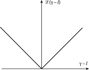
  FIGURE 11.2 Linear modulo loss function.

  

  FIGURE 11.3 Quadratic loss function.

  

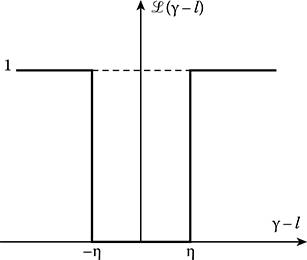
  FIGURE 11.4 Rectangle loss function.

• Quadratic loss function (see Figure 11.3)

  ℒ(γ,l)=(γ−l)2;⁢(11.25)

• Rectangle loss function (see Figure 11.4)

  ℒ(γ,l)={0if|γ−l|<η,η>0,1if|γ−l|>η,η>0.⁢(11.26)

In general, there may be a factor on the right side of loss functions given by (11.23) through (11.24). These functions are the symmetric functions of difference |γ − l|. In doing so, deviations of the parameter estimate with respect to the true value of estimated random process parameter are undesirable. In addition, there are some application problems when the observer ignores the sign of estimate. In this case, the loss function is not symmetric.

Based on the random nature of estimations y and random process parameter l, the losses are random for any decision-making rules and cannot be used to characterize an estimate quality. To characterize an estimate quality, we can apply the mathematical expectation of the loss function that takes into consideration all incorrect solutions and relative frequency of their appearance. Choice of the mathematical expectation to characterize a quality of estimate, not another statistical characteristic, is rational but a little bit arbitrary. The mathematical expectation (conditional or unconditional) of the loss function is called the risk (conditional or unconditional). Conditional risk is obtained by averaging the loss function over all possible values of multidimensional sample of the observed data that are characterized by the conditional pdf p(X|l)

As we can see from (11.27), the preferable estimations are the estimations with minimal conditional risk. However, at various values of the estimated random process parameter l, the conditional risk will have different values. For this reason, the preferable decision-making rules can be various, too. Thus, if we know the a priori pdf of the estimated parameter, then it is worthwhile to define the best decision-making rule for the definition of estimation based on the condition of the unconditional average minimum risk, which can be written in the following form:

where p(X) is the pdf of the observed data sample.

Estimations obtained by the criterion of minimum conditional and unconditional average risk are called the conditional and unconditional Bayes estimates. The unconditional Bayes estimate is often called the Bayes estimate. Furthermore, we will understand that for the Bayes estimate γ_m of the parameter l the estimate ensuring the minimum average risk at the given loss function is ℒ(γ, l). The minimal value of average risk corresponding to the Bayes estimate is called the Bayes risk

Here, the averaging is carried out by samples (digital signal processing) of the observed data X or by realizations x(t) (analog signal processing). The average risk can be determined for any given decision-making rule and because of the definition of Bayes estimate the following condition is satisfied forever:

Computing the average risk by (11.28) for different estimations and comparing each of these risks with Bayes risk, we can evaluate and conclude how one estimate can be better compared to another estimate and that the best estimate is the one close to the optimal Bayes estimate. Since the conditional or unconditional risk has a varying physical sense depending on the shape and physical interpretation of the loss function ££(y, l), the sense of criterion of optimality depends on the shape of the loss function, too.

The pdf p(X) is the nonnegative function. For this reason, a minimization of (11.28) by y at the fixed sample of observed data is reduced to minimization of the function

called the a posteriori risk. If the a posteriori risk ℛ_post(γ) is differentiated by γ, then the Bayes estimate γ_m can be defined as a solution of the following equation:

To ensure a global minimum (minimum minimorum) of the a posteriori risk ℛ_post(γ), we need to use the root square.

The criterion of minimum average risk is based on the knowledge of the total a priori information about the estimated parameter, which gives the answer to the question about how we can use all a priori information to obtain the best estimate. However, the absence of the total a priori information about the estimated parameter that takes place in the majority of applications leads us to definite problems (a priori problems) with applying the methods of the theory of statistical estimations. Several approaches are found to solve the problems of definition of the optimal estimations at the unknown a priori distribution of estimated parameters. One of them is based on definition of the Bayes estimations that are invariant with respect to the sufficiently wide class of a priori distributions. In other problems, we are limited by a choice of estimation based on the minimization of the conditional risk or we make some assumptions with respect to a priori distribution of estimated parameters. The least favorable distribution, with the Bayes risk at the maximum, is considered as the a priori distribution of estimated parameters; the obtained estimation of the random process parameter is called the minimax estimate. The minimax estimate defines the upper bound of the Bayes risk that is called the minimax risk. In spite of the fact that minimax estimate can generate heavy losses compared to other possible estimate, it can be useful if losses under the most unfavorable a priori conditions are avoided.

In accordance with the definition, the minimax estimate can be defined in the following way. In the case of a priori distribution of estimated parameter in accordance with the given loss function, we need to define the Bayes estimate γ_m = γ_m[x(t)]. After that we select such a priori distribution of estimated parameter, at which the minimal value of the average risk (Bayes risk) reaches the maximum. The Bayes estimate will be minimax at such a priori distribution. We need to note that a rigorous definition of the least favorable a priori distribution of estimated parameter is related to great mathematical problems. However, in the majority of applications, including the problems of random parameter estimations, the least favorable pdf is the uniform distribution within the limits of the given interval.

11.5 Bayesian Estimates for Various Loss Functions

Now, we discuss the properties of Bayes estimations for some loss functions mentioned previously.

11.6 Summary and Discussion

In many practical applications, the estimate criteria are selected based on assumptions about the purpose of estimate. At the same time, during the process design, choosing a definite estimate criteria is of great interest because such approach allows us to understand more clearly the essence and characteristic property of the problem to estimate the random process parameter, which is very important, giving us a possibility to define the problem of valid selection of the estimate criterion more fairly. Owing to the finite time of observation and presence of noise and interference concurrent to observation, specific errors in the course of estimate definition arise. These errors are defined both by the quality performance and by conditions under which an estimation process is carried out. In general, the requirement of minimization of estimation error by value does not depend on just one assumption. However, if the criterion of estimation is given, the quality performance is measured based on this criterion. Then the problem of obtaining the optimal estimation is reduced to a definition of solution procedure that minimizes or maximizes the quality performance. In doing so, the parameter estimate must be close, in a certain sense, to the true value of estimated parameter and the optimal estimate must minimize this measure of closeness in accordance with the chosen criterion.

In theory, for statistical parameter estimation, two types of estimates are used: the interval estimations based on the definition of confidence interval, and the point estimation, that is, the estimate defined at the point. Employing the interval estimations, we need to indicate the interval, within the limits of which there is the true value of unknown random process parameter with the probability that is not less than the predetermined value. This predetermined probability is called the confidence factor and the indicated interval of possible values of estimated random process parameter is called the confidence interval. The upper and lower bounds of the confidence interval, which are called the confidence limits, and the confidence interval are the functions to be considered during digital signal processing (a discretization) or during analog signal processing (continuous function). of the received realization x (t). In the case of point estimation, we assign one parameter value to the unknown parameter from the interval of possible parameter values; that is, some value is obtained based on the analysis of the received realization x (t) and we use this value as the true value of the evaluated parameters.

In addition to the procedure of analysis of the estimation random process parameter based on an analysis of the received realization x (t), a sequential estimation method is used. Essentially, this method is used for the sequential statistical analysis to estimate the random process parameter. The basic idea of sequential estimation is to define the time of analysis of the received realization x (t), within the limits of which we are able to obtain the estimate of parameter with the preset criteria for reliability. In the case of the point estimate, the root-mean-square deviation of estimate or other convenience function characterizing a deviation of estimate from the true value of estimated random process parameter can be considered as the measure of reliability. From a viewpoint of interval sequential estimation, the estimate reliability can be defined using a length of the confidence interval with the given confidence coefficient.

To make the point estimation means that some number from the interval of possible values of the estimated random process parameter must correspond to each possible received realization. This number is called the point estimate. Owing to the random character of the point estimate of random process parameter, it is characterized by the conditional pdf. This is a general and total characteristic of the point estimate. A shape of this pdf defines a quality of point estimate definition and, consequently, all properties of the point estimate.

There are several approaches to define the properties of the point estimations: (a) It is natural to try to define such point estimate that the conditional pdf would be grouped very close to the estimate value; (b) it is desirable that while increasing the observation interval, the estimation would coincide with or approach stochastically the true value of the estimated random process parameter (in this case, we can say that the estimate is the consistent estimate); (c) the estimate must be unbiased or, in an extreme case, asymptotically unbiased; (d) the estimate must be the best by some criterion; for example, it must be characterized by minimal values of dispersion or variance at zero or constant bias; and (e) the estimate must be a statistically sufficient measure.

Based on the random character of the observed realization, we can expect errors in any decision-making rules; that is, such a decision does not coincide with the true value of a parameter By applying various decision-making rules, different errors will appear with different levels of probability. Since the nonzero probability of error exists forever, we need to characterize the quality of different estimations in one way or another. For this purpose, the loss function is introduced in the theory of decisions. This function defines a definite loss for each combination from the decision and parameter. The physical sense of the loss function is the following. A definite nonnegative weight is assigned to each incorrect decision. In doing so, depending on targets, for which the estimate is defined, the most undesirable decisions are assigned the greatest weights. A choice of definite loss function is made depending on a specific problem of estimation of the random process parameter. There is no general decision-making rule to select the loss function. Each decision-making rule is selected based on a subjective principle. Any arbitrariness with selecting losses leads to definite difficulties with applying the theory of statistical decisions. The following types of loss functions are widely used in practice: the simple loss function, the linear modulo loss function, the quadratic loss function, and the rectangle loss function.

References

1. Kay, S.M. 2006. Intuitive Probability and Random Processes Using MATLAB. New York: Springer + Business Media, Inc.

2. Govindarajulu, Z. 1987. The Sequential Statistical Analysis of Hypothesis Testing Point and Interval Estimation, and Decision Theory. (American Series in Mathematical and Management Science). New York: American Sciences Press, Inc.

3. Sieqmund, D. 2010. Sequential Analysis: Test and Confidence Intervals. (Springer Series in Statistics). New York: Springer + Business Media, Inc.

4. Kay, S.M. 1993. Fundamentals of Statistical Signal Processing: Estimation Theory. Upper Saddle River, NJ: Prentice Hall, Inc.

5. Cramer, H. 1946. Mathematical Methods of Statistics. Princeton, NJ: Princeton University Press.

6. Cramer, H. and M.R. Leadbetter. 2004. Stationary and Related Stochastic Processes: Sample Function Properties and Their Applications. Mineola, NY: Dover Publications.