Chapter 12 Estimation of Mathematical Expectation

Search in book...
Toggle Font Controls
Create new playlist

Name your new playlist

Playlist description (optional)
Sign In

Email address

Password

Forgot Password?

or

Continue with Facebook

Continue with Google
Sign Up

Full Name

Email address

Confirm Email Address

Password

or

Continue with Facebook

Continue with Google

Let the analyzed Gaussian stochastic process ξ(t) possess the mathematical expectation defined as

$E (t) = E_{0} s (t) (12.1)$

the correlation function R(t₁, t₂), and be observed within the limits of the finite time interval [0, T]. We assume that the law of variation of the mathematical expectation s(t) and correlation function R(t₁, t₂) are known. Thus, the received realization takes the following form:

$x (t) = E (t) + x_{0} (t) = E_{0} s (t) + x_{0} (t), 0 \leq t \leq T, (12.2)$

where

$x_{0} (t) = x (t) - E (t) (12.3)$

is the centered Gaussian stochastic process. The problem with estimating the mathematical expectation is correlated to the problem with estimating the amplitude E(t) of the deterministic signal in the additive Gaussian noise.

The pdf functional of the Gaussian process given by (12.2) takes the following form:

$F [x (t) | E_{0}] = B_{0} \exp {- 0.5 \int_{0}^{T} \int_{0}^{T} ϑ (t_{1}, t_{2}) [x (t_{1}) - E_{0} s (t_{1})] \times [x (t_{2}) - E_{0} s (t_{2}) d t_{1} d t_{2}]} . (12.4)$

where B₀ is the factor independent of the estimated parameter E₀; the function

$ϑ (t_{1}, t_{2}) = ϑ (t_{2}, t_{1}) (12.5)$

is defined from the integral equation

$\int_{0}^{T} R (t_{1}, t) ϑ (t_{1}, t_{2}) d t = δ (t_{2} - t_{1}) . (12.6)$

Introduce the following function:

$υ (t) = \int_{0}^{T} s (t_{1}) ϑ (t_{1}, t) d t_{1}, (12.7)$

which is a solution of the following integral equation:

$\int_{0}^{T} R (t, τ) υ (τ) d τ = s (t) . (12.8)$

Since the received realization of the Gaussian stochastic process does not depend on the current value of estimation E₀, the pdf functional of Gaussian stochastic process can be written in the following form:

$F [x (t) | E_{0}] = B_{1} \exp {E_{0} \int_{0}^{T} x (t) υ (t) d t - 0.5 E_{0}^{2} \int_{0}^{T} s (t) υ (t) d t}, (12.9)$

where B₁ is the factor independent of the estimated parameter E₀.

As applied to analysis of the stationary stochastic process, we can write

${\begin{array}{l} s (t) = 1, \\ R (t_{1}, t_{2}) = R (t_{2} - t_{1}) = R (t_{1} - t_{2}) . \end{array} (12.10)$

In doing so, the function υ(t) and the pdf functional are determined as

$\int_{0}^{T} R (t - τ) υ (τ) d τ = 1; (12.11)$

$F [x (t) | E_{0}] = B_{1} \exp {E_{0} \int_{0}^{T} x (t) υ (t) d t - 0.5 E_{0}^{2} \int_{0}^{T} υ (t) d t} . (12.12)$

In practice, the stationary stochastic processes occur very often and their correlation functions can be written in the following form:

$R (τ) = σ^{2} \exp {- α | τ |}, (12.13)$

$R (τ) = σ^{2} \exp {- α | τ |} [\cos ω_{1} τ \frac{α}{ω_{1}} \sin ω_{1} | τ |], (12.14)$

where σ² is the variance of stationary stochastic process. These correlation functions correspond to the stationary stochastic processes obtained as a result of excitation of the RC-circuit, α = (RC)⁻¹, and the RLC-circuit, $ω_{1}^{2} = ω_{0}^{2} - α^{2}, ω_{0}^{2} = {(L C)}^{- 1} > α = R {(2 L)}^{- 1}$ inputs by the “white” noise.

Solution of (12.8) for the correlation functions given by (12.13) and (12.14) takes the following form, respectively:

$υ (t) = \frac{α}{2 σ^{2}} [s (t) - α^{- 2} s ″ (t)] + \frac{1}{σ^{2}} {[s (0) - α^{- 1} s' (0)] δ (t) + [s (T) + α^{- 1} s' (T)] δ (T - t)}, (12.15)$

$υ (t) = \frac{1}{4 σ^{2} α ω_{0}^{2}} [s ″ ″ (t) + 2 (ω_{0}^{2} - 2 α^{2}) s ″ (t) + ω_{0}^{4} s (t)] + \frac{1}{2 σ^{2} α ω_{0}^{2}} {[s ″' (0) + (ω_{0}^{2} - 4 α^{2}) s' (0) + 2 α ω_{0}^{2} s (0)] δ (t) - [s ″' (T) + (ω_{0}^{2} - 4 α^{2}) s' (T) - 2 α ω_{0}^{2} s (T)] δ (t - T) + [s ″ (0) - 2 α s' (0) + ω_{0}^{2} s (0)] δ' (t) - [s ″ (T) + 2 α s' (T) + ω_{0}^{2} s (T)] δ' (t - T)} . (12.16)$

The notations s′(t), s″(t), s′″(t), s″″(t) mean the derivatives of the first, second, third, and fourth order with respect to t, respectively. If the function s(t) and its derivatives at t = 0 and t = T become zero, then (12.15) and (12.16) have a simple form. As applied to stochastic process at s(t) = 1 = const, (12.15) and (12.16) have the following form:

$υ (t) = \frac{α}{2 σ^{2}} + \frac{1}{σ^{2}} [δ (t) + δ (T - t)], (12.17)$

$υ (t) = \frac{ω_{0}^{2}}{4 α σ^{2}} + \frac{1}{σ^{2}} [δ (t) + δ (t - T)] + \frac{1}{2 α σ^{2}} [δ' (t) - δ' (t - T)] . (12.18)$

The following spectral densities

$S (ω) = \frac{2 α σ^{2}}{α^{2} + ω^{2}} (12.19)$

and

$S (ω) = \frac{4 α σ^{2} (ω_{1}^{2} + α^{2})}{ω^{4} - 2 ω^{2} (ω_{1}^{2} - α^{2}) + {(ω_{1}^{2} + α^{2})}^{2}} (12.20)$

correspond to the correlation functions given by (12.13) and (12.14), respectively. It is necessary to note that there is no general procedure to solve (12.8). However, if the correlation function of stochastic process depends on the absolute value of difference of arguments |t₂ − t₁| and the observation time T is much more than the correlation interval defined as

$τ_{cor} = \frac{1}{σ^{2}} \int_{0}^{\infty} | R (τ) | d τ = \int_{0}^{\infty} | ℛ (τ) | d τ, (12.21)$

where

$ℛ (τ) = \frac{R (τ)}{σ^{2}} (12.22)$

is the normalized correlation function, and the function s(t) and its derivatives at t = 0 and t = T become zero, it is possible to define the approximate solution of the integral equation (12.8) using the Fourier transform. Applying the Fourier transform to the left and right side of the following equation

$\int_{- \infty}^{\infty} R (t - τ) \tilde{υ} (τ) d τ = s (t), (12.23)$

it is not difficult to use the inverse. Fourier transform in order to obtain

$\tilde{υ} (t) = \frac{1}{2 π} \int_{- \infty}^{\infty} \frac{S (ω)}{S (ω)} \exp {j ω t} d ω . (12.24)$

where

S (ω) is the Fourier transform of the correlation function R(τ)
S(ω) is the Fourier transform of mathematical expectation of the function s (t), which can be defined as

$S (ω) = \int_{- \infty}^{\infty} R (τ) \exp {- j ω τ} d τ, (12.25)$

$S (ω) = \int_{- \infty}^{\infty} s (t) \exp {- j ω t} d t . (12.26)$

The inverse Fourier transform gives us the following formulae:

$R (τ) = \frac{1}{2 π} \int_{- \infty}^{\infty} S (ω) \exp {j ω τ} d ω, (12.27)$

$s (t) = \frac{1}{2 π} \int_{- \infty}^{\infty} S (ω) \exp {j ω τ} d ω . (12.28)$

If the function s(t) and its derivatives do not become zero at t = 0 and t = T and the function S(ω) is a ratio of two polynomials of pth and dth orders, respectively, with respect to ω² and d > p, then there is a need to add the delta function δ(t) and its derivative δ′(t) taken at t = 0 and t = T. Thus, there is a need to define the solution for Equation 12.8 in the following form:

$υ (t) = \tilde{υ} (t) + \sum_{μ = 0}^{d - 1} [b_{μ} δ^{μ} (t) + c_{μ} δ^{μ} (t - T)] . (12.29)$

Here, the coefficients b_μ and c_μ are defined from the solutions of equations obtained under the substitution of (12.29) in (12.8); δ_μ(t) is the delta function derivative of μth order with respect to the time.

In the case of stationary stochastic process, we have s(t) = 1. In this case, the spectral density takes the following form:

$S (ω) = 2 π δ (ω) . (12.30)$

From (12.24) and (12.29), we have

$υ (t) = S^{- 1} (ω = 0) + \sum_{μ = 0}^{d - 1} [b_{μ} δ^{μ} (t) + c_{μ} δ^{μ} (t - T)] . (12.31)$

As applied to the stationary stochastic process with the spectral density given by (12.19), we have that d = 1. For this reason, we can write

$υ (t) = \frac{α}{2 σ^{2}} + b_{0} δ (t) + c_{0} δ (t - T) . (12.32)$

Substituting (12.13) and (12.32) into (12.5), we obtain

$0.5 [α \int_{0}^{T} \exp {- α | t - τ |} d τ + b_{0} σ^{2} \exp {- α t} + c_{0} σ^{2} \exp {- α (T - t)}] = 1. (12.33)$

Dividing the integration intervals on two intervals, namely, 0 ≤ τ ≤ t and t ≤ τ ≤ T, after integration we obtain

$(b_{0} σ^{2} - 1) \exp {- α t} + (c_{0} σ^{2} - 1) \exp {- α (t - T)} = 0. (12.34)$

This equality is correct if the coefficient of the terms exp{−αt} and exp{−α(t − T)} is equal to zero, that is, b₀ = c₀ = σ⁻². Substituting b₀ and c₀ into (12.32), we obtain the formula given by (12.17).

Now, consider the exponential function in (12.9). The formula

$ρ_{1}^{2} = \int_{0}^{T} s (t) υ (t) d t (12.35)$

is the deterministic component or, in other words, the signal when the estimated parameter E₀ = 1. The random component

$\int_{0}^{T} x_{0} (t) υ (t) d t (12.36)$

is the noise component. The variance of the noise component taking into consideration (12.8) is defined as

$〈 {[\int_{0}^{T} x_{0} (t) υ (t) d t]}^{2} 〉 = \int_{0}^{T} \int_{0}^{T} 〈 x_{0} (t_{1}) x_{1} (t_{2}) 〉 υ (t_{1}) υ (t_{2}) d t_{1} d t_{2} = \int_{0}^{T} s (t) υ (t) d t = ρ_{1}^{2} . (12.37)$

As we can see from (12.37), $ρ_{1}^{2}$ is the ratio between the power of the signal and the power of the noise. Because of this, we can say that (12.37) is the signal-to-noise ratio (SNR) when the estimated parameter value E₀ = 1.

12.2 Maximum Likelihood Estimate of Mathematical Expectation

Consider the conditional functional given by (12.9) of the observed stochastic process. Solving the likelihood equation with respect to the parameter E, we obtain the mathematical expectation estimate

$E_{E} = \frac{\int_{0}^{T} x (t) υ (t) d t}{\int_{0}^{T} s (t) υ (t) d t} . (12.38)$

As applied to analysis of stationary stochastic process, (12.38) becomes simple, namely,

$E_{E} = \frac{\int_{0}^{T} x (t) υ (t) d t}{\int_{0}^{T} υ (t) d t} . (12.39)$

In doing so, at the condition $T τ_{cor}^{- 1} \to \infty$ we can neglect the values of stochastic process and its derivatives at t = 0 and t = T under estimation of the mathematical expectation; that is, in other words, we can think that the following approximation is correct:

$υ (t) = S^{- 1} (ω = 0) . (12.40)$

In this case, we obtain the asymptotical formula for the mathematical expectation estimate of stationary stochastic process, namely,

$E_{E} = \lim_{T \to \infty} \frac{1}{T} \int_{0}^{T} x (t) d t, (12.41)$

which is widely used in the theory of stochastic processes to define the mathematical expectation of ergodic stochastic processes with arbitrary pdf. At the large and finite values $T τ_{cor}^{- 1}$ , we can neglect an effect of values of the stochastic process and its derivatives at t = 0 and t = T on the mathematical expectation estimate. As a result, we can write

$E_{E} \approx \frac{1}{T} \int_{0}^{T} x (t) d t . (12.42)$

Images

FIGURE 12.1 Optimal structure to define the mathematical expectation estimate.

Although the obtained formulae for the mathematical expectation estimate are optimal in the case of Gaussian stochastic process, these formulae will be optimal for the stochastic process differed from the Gaussian pdf in the class of linear estimations. Equations 12.38 and 12.39 are true if the a priori interval of changes of the mathematical expectation is not limited. Equation 12.38 allows us to define the optimal device structure to estimate the mathematical expectation of the stochastic process (Figure 12.1). The main function is the linear integration of the received realization x (t). with the weight υ(t) that is defined based on the solution of the integral equation (12.8). The decision device issues the output process at the instant t = T. To obtain the current value of the mathematical expectation estimate, the limits of integration in (12.38) must be t − T and t, respectively. Then the parameter estimation is defined as

$E_{E} (t) = \frac{\int_{t - T}^{t} x (τ) υ (τ) d τ}{\int_{t - T}^{t} s (τ) υ (τ) d τ} . (12.43)$

The weight integration can be done by the linear filter with corresponding impulse response. For this purpose, we introduce the function

$υ (τ) = h (t - τ) or h (τ) = υ (t - τ) (12.44)$

and substitute this function into (12.43) instead of υ(t) introducing a new variable t − τ = z. Then (12.43) can be transformed to the following form:

$E_{E} (t) = \frac{\int_{0}^{T} x (t - z) h (z) d z}{\int_{0}^{T} s (t - z) h (z) d z} . (12.45)$

The integrals in (12.45) are the output responses of the linear filter with the impulse response h (t) given by (12.44) when the filter input is excited by x (t) and s (t), respectively. The mathematical expectation of estimate

$〈 E_{E} 〉 = \frac{1}{ρ_{1}^{2}} \int_{0}^{T} 〈 x (t) 〉 υ (t) d t = E_{0}, (12.46)$

that is, the estimate of the maximum likelihood of the mathematical expectation of stochastic process is both the conditionally and unconditionally unbiased estimate. The conditional variance of the mathematical expectation estimate can be presented in the following form:

$Var {E_{E} | E_{0}} = 〈 E_{E}^{2} 〉 - {〈 E_{E} 〉}^{2} = \frac{1}{ρ_{1}^{4}} \int_{0}^{T} \int_{0}^{T} 〈 x_{0} (t_{1}) x_{0} (t_{2}) 〉 υ (t_{1}) υ (t_{2}) d t_{1} d t_{2} = ρ_{1}^{- 2}, (12.47)$

that is, the variance of estimate is unconditional. Since, according to (12.38), the integration of Gaussian stochastic process is a linear operation, the estimate E_E is subjected to the Gaussian distribution.

Let the analyzed stochastic process be a stationary process and possess the correlation function given by (12.13). Substituting instead of the function υ(t) its value from (12.17) into (12.47) and integrating with delta functions, we obtain

$Var {E_{E}} = \frac{2 σ^{2}}{2 + (T / τ_{cor})} = \frac{2 σ^{2}}{2 + α T} = \frac{2 σ^{2}}{2 + p}, (12.48)$

where p is a ratio between the time required to analyze the stochastic process and the correlation interval of the same stochastic process. In doing so, according to (12.38), the formula for the optimal estimate takes the following form:

$E_{E} = \frac{x (0) + x (T) + α \int_{0}^{T} x (t) d t}{2 + p} . (12.49)$

If p ≫ 1, we have

$Var {E_{E}} \approx \frac{2 σ^{2}}{p} . (12.50)$

Formulae (12.48) and (12.49) can be obtained without determination of the pdf functional. For this purpose, the value defined by the following equation:

$E * = \int_{0}^{T} h (t) x (t) d t (12.51)$

can be considered as the estimate. Here h(t) is the weight function defined based on the condition of unbiasedness of the estimate that is equivalent to

$\int_{0}^{T} h (t) d t = 1, (12.52)$

and minimization of the variance of estimate,

$Var {E *} = \int_{0}^{T} \int_{0}^{T} h (t_{1}) h (t_{2}) R (t_{1}, t_{2}) d t_{1} d t_{2} . (12.53)$

Transform the formula for the variance of estimate into a convenient form. For this purpose, introduce new variables in the double integral, namely,

$\begin{matrix} τ = t_{2} - t_{1} & and & t_{1} = z, \end{matrix} (12.54)$

and change the order of integration. Taking into consideration that R(x) = R(−t), we obtain

$Var {E *} = 2 \int_{0}^{T} R (τ) \int_{0}^{T - τ} h (z) h (z + τ) d z d τ . (12.55)$

As was shown in Ref. [1], a definition of optimal form of the weight function h(t) is reduced to a solution of the integral Wiener-Hopf equation

$\int_{0}^{T} h (τ) R (τ - s) d τ - {Var}_{min} {E} = 0, 0 \leq s \leq T, (12.56)$

where Var_min{E} is the minimal estimate variance, jointly with the condition given by (12.52). However, the solution of (12.56) is complicated.

Define the formula for an optimal estimate of mathematical expectation of the stationary sto-chastic process possessing the correlation function given by (12.14) and weight function given by (12.18). Substituting (12.18) into the formula for mathematical expectation estimate of the stochastic process defined as (12.38) and calculating the corresponding integrals, the following is obtained:

$E_{E} = \frac{\frac{1}{T} \int_{0}^{T} x (t) d t + \frac{2 α}{ω_{0}^{2} T} [x (0) + x (T)] + \frac{1}{ω_{0}^{2} T} [x' (0) - x' (t)]}{1 + \frac{4 α}{ω_{0}^{2} T}} . (12.57)$

In doing so, the variance of the mathematical expectation estimate is defined as

$Var {E_{E}} = \frac{4 α σ^{2}}{ω_{0}^{2} T + 4 α} . (12.58)$

If α ≪ ω₀ and ω₀T ≫ 1, the formula for the mathematical expectation estimate of the stationary Gaussian stochastic process transforms to the well-known formula of the mathematical expectation definition of the ergodic stochastic process given by (12.42), and the variance of the mathematical expectation estimate is defined as

$Var {E_{E}} \approx \frac{4 α σ^{2}}{ω_{0}^{2} T} . (12.59)$

At ω₁ = 0 (ω₀ = α), the correlation function given by (12.14), can be transformed into the following form

$R (τ) = σ^{2} \exp {- α | τ |} (1 + α | τ |), τ_{cor} = \frac{2}{α} (12.60)$

by limiting process. In particular, the given correlation function corresponds to the stationary stochastic process at the output of two RC circuits connected in series when the “white” noise excites the input. In this case, the formulae for the mathematical expectation estimate and variance take the following form:

$E_{E} = \frac{\frac{1}{T} \int_{0}^{T} x (t) d t + \frac{2}{α T} [x (0) + x (T)] + \frac{1}{α^{2} T} [x' (0) - x' (T)]}{1 + \frac{4}{α T}}, (12.61)$

$Var {E_{E}} = \frac{4 σ^{2}}{α T + 4} . (12.62)$

Relationships between the definition of the estimate and the estimate variance of the mathematical expectation of the stochastic processes with other types of correlation functions can be defined analogously.

As we assumed before, the a priori domain of definition of the mathematical expectation is not limited. Thus, we consider a domain of possible values of the mathematical expectation as a function of the mathematical expectation estimate. Let the a priori domain of definition of the math-ematical expectation be limited both by the upper bound and by the lower bound, that is,

$E_{L} \leq E \leq E_{0} . (12.63)$

In the considered case, the mathematical expectation estimate Ê cannot be outside the considered interval given by (12.63), even though it is defined as a position of the absolute maximum of the likelihood functional logarithm (12.9). The likelihood functional logarithm reaches its maximum at E = E_E. As a result, when E_E ≤ E_L the likelihood functional logarithm becomes a monotonically decreasing function within the limits of the interval [E_L, E_U] and reaches its maximum value at E= E_L. If E_E ≥ E_U, the likelihood functional logarithm becomes a monotonically increasing function within the limits of the interval [E_L, E_U] and, consequently, reaches its maximum value at E = E_U. Thus, in the case of the limited a priori domain of definition of the mathematical expectation, the estimate of mathematical expectation of stochastic process can be presented in the following form:

$\hat{E} = {\begin{array}{l} E_{U} & if & E_{E} > E_{U}, \\ E_{E} & if & E_{L} \leq E_{E} \leq E_{U}, \\ E_{L} & if & E_{E} < E_{L} . \end{array} (12.64)$

Taking into consideration the last relationship, the structure of optimal device for the mathemat-ical expectation estimate determination in the case of the limited a priori domain of mathematical expectation definition can be obtained by the addition of a linear limiter with the following characteristic:

$g (z) = {\begin{array}{l} E_{U} & if & z > E_{U}, \\ z & if & E_{L} \leq z \leq E_{U}, \\ E_{L} & if & z < E_{L} \end{array} (12.65)$

to the circuit shown in Figure 12.1. Using the well-known relationships [2] to transform the Gaussian random variable pdf of by a nonlinear inertialess system with the chain characteristic g (z), we can define the conditional pdf of the mathematical expectation estimate as follows:

$ρ (\hat{E} | E_{0}) = {\begin{array}{l} P_{L} δ (\hat{E} - E_{L}) + P_{U} δ (\hat{E} - E_{U}) + \frac{1}{\sqrt{2 π Var (E_{E} | E_{0})}} \exp {- \frac{{(\hat{E} - E_{0})}^{2}}{2 Var (E_{E} | E_{0})}} \\ 0, at \hat{E} < E_{L}, \hat{E} > E_{U} . \end{array} at E_{L} \leq E_{E} \leq E_{U}, (12.66)$

Here

${\begin{array}{l} P_{L} = 1 - Q (\frac{E_{L} - E_{0}}{\sqrt{Var (E_{E} | E_{0})}}), \\ P_{U} = Q (\frac{E_{L} - E_{0}}{\sqrt{Var (E_{E} | E_{0})}}); \end{array} (12.67)$

where

$Q (z) = \frac{1}{\sqrt{2 π}} \int_{z}^{\infty} \exp {- 0.5 y^{2}} d y (12.68)$

is the Gaussian Q function [3, 4]; Var(E_E|E₀) is the variance given by (12.47). The conditional bias is defined as

$b (\hat{E} | E_{0}) = 〈 \hat{E} 〉 - E_{0} = \int_{- \infty}^{\infty} (\hat{E} - E_{0}) p (\hat{E} | E_{0}) d \hat{E} = P_{L} (E_{L} - E_{0}) + P_{U} (E_{U} - E_{0}) + \sqrt{\frac{Var (E_{E} | E_{0})}{2 π}} {\exp [- \frac{{(E_{L} - E_{0})}^{2}}{2 Var (E_{E} | E_{0})}] - \exp [- \frac{{(E_{U} - E_{0})}^{2}}{2 Var (E_{E} | E_{0})}]} . (12.69)$

Thus, in the case of the limited a priori domain of possible values of the mathematical expectation of stochastic process, the maximum likelihood estimate of the stochastic process mathematical expectation is conditionally biased. However, at small variance values of the maximum likelihood estimate of stochastic process mathematical expectation, that is, Var(E_E|E₀) → 0, as it follows from (12.67) and (12.69), we obtain the asymptotical expression

$\lim_{Var (E_{E} | E_{\begin{array}{l} 0 \end{array}}) \to 0} b (E_{E} | E_{0}) = 0; (12.70)$

that is, at Var(E_E|E₀) → 0, the maximum likelihood estimate of mathematical expectation of sto-chastic process is asymptotically unbiased. At the high variance values of the maximum likelihood estimate of stochastic process mathematical expectation, that is, Var(E_E|E₀) → ∞, the bias of the maximum likelihood estimate of stochastic process mathematical expectation tends to approach

$b (E_{E} | E_{0}) = 0.5 (E_{L} + E_{U} - 2 E_{0}) . (12.71)$

The conditional dispersion of the maximum likelihood estimate of stochastic process mathematical expectation is defined as

$D (E_{E} | E_{0}) = \int_{- \infty}^{\infty} {(\hat{E} - E_{0})}^{2} f (E_{E} | E_{0}) d \hat{E} = P_{L} {(E_{L} - E_{0})}^{2} + P_{U} {(E_{L} - E_{0})}^{2} + Var (1 - P_{U} - P_{L}) + \sqrt{\frac{Var (E_{E} | E_{0})}{2 π}} {(E_{L} - E_{0}) \exp [- \frac{{(E_{L} - E_{0})}^{2}}{2 Var (E_{E} | E_{0})}] - (E_{U} - E_{0}) \exp [- \frac{{(E_{U} - E_{0})}^{2}}{2 Var (E_{E} | E_{0})}]} . (12.72)$

At small variance values of the maximum likelihood estimate of stochastic process mathematical expectation

$\frac{Var (E_{E} | E_{0})}{E_{U} - E_{L}} ≪ 1 and E_{L} < E < E_{U} (12.73)$

if the limiting process is carried out at E_L → − ∞ and E_U → ∞, the conditional dispersion of the maximum likelihood estimate of stochastic process mathematical expectation coincides with the variance of estimate given by (12.47). If the true value of the mathematical expectation coincides with one of two bounds of the a priori domain of possible values of the mathematical expectation, then the following approximation is true:

$D (E_{E} | E_{0}) \approx 0.5 Var (E_{E} | E_{0}); (12.74)$

that is, the dispersion of estimate is twice as less compared to the unlimited a priori domain case. With increasing variance of the maximum likelihood estimate of stochastic process mathematical expectation Var(E_E|E₀) → ∞, the conditional dispersion of the maximum likelihood estimate of the stochastic process mathematical expectation tends to approach the finite value since P_L = P_U = 0.5

$D (E_{E} | E_{0}) \to 0.5 [{(E_{L} - E_{0})}^{2} + {(E_{U} - E_{0})}^{2}], (12.75)$

whereas the dispersion of the maximum likelihood estimate of stochastic process mathematical expectation within the unlimited a priori domain of possible values of the maximum likelihood estimate of stochastic process mathematical expectation is increased without limit as Var(E_E|E₀) → ∞. It is important to note that although the bias and dispersion of the maximum likelihood estimate of stochastic process mathematical expectation are defined as the conditional values, they are never-theless independent of the true value of the mathematical expectation E₀ and are the unconditional estimates simultaneously.

Determine the unconditional bias and dispersion of maximum likelihood estimate of stochastic process mathematical expectation in the case of the limited a priori domain of possible estimate values. For this purpose, it is necessary to average the conditional characteristics given by (12.69) and (12.72) with respect to possible values of estimated parameter, assuming that the a priori pdf of estimated parameter is uniform within the limits of the interval [E_L, E_U]. In this case, we observe that the unconditional estimate is unbiased, and the unconditional dispersion is determined in the following form:

$D (\hat{E}) = Var {1 - 2 Q [\frac{E_{U} - E_{L}}{\sqrt{Var (E_{L} | E_{0})}}]} + \frac{2}{3} {(E_{U} - E_{L})}^{2} Q [\frac{E_{U} - E_{L}}{\sqrt{Var (E_{E} | E_{0})}}] - \frac{2 Var (E_{E} | E_{0}) \sqrt{Var (E_{E} | E_{0})}}{3 \sqrt{2 π} (E_{U} - E_{L})} {1 - \exp {- \frac{{(E_{U} - E_{L})}^{2}}{2 Var (E_{E} | E_{0})}}} - \frac{2 \sqrt{Var (E_{E} | E_{0})} (E_{U} - E_{L})}{3 \sqrt{2 π}} \exp {- \frac{{(E_{U} - E_{L})}^{2}}{2 Var (E_{E} | E_{0})}} . (12.76)$

At the same time, it is not difficult to see that at small values of the variance, that is, Var(E_E|E₀) → 0, the unconditional dispersion transforms into a dispersion of the estimate obtained under the unlimited a priori domain of possible values, D (Ê) → Var(E_E|E₀). Otherwise, at high values of variance, that is, Var(E_E|E₀) → ∞, the dispersion of the estimate given by (12.47) increases without limit and the unconditional dispersion given by (12.76) has a limit equal to the average square of the a priori domain of possible values of the estimate, that is, (E_U − E_L)²/3.

12.3 Bayesian Estimate of Mathematical Expectation: Quadratic Loss Function

As before, we analyze the realization x(t) of stochastic process given by (12.2). The a posteriori pdf of estimated stochastic process parameter E can be presented in the following form:

$p_{post} (E) = \frac{p_{prior} (E) \exp {E \int_{0}^{T} x (t) υ (t) d t - \frac{E^{2}}{2} \int_{0}^{T} s (t) υ (t) d t}}{\int_{- \infty}^{\infty} p_{prior} (E) \exp {E \int_{0}^{T} x (t) υ (t) d t - \frac{E^{2}}{2} \int_{0}^{T} s (t) υ (t) d t} d E}, (12.77)$

where

p_prior(E) is the a priori pdf of estimated stochastic process parameter
υ(t) is the solution of the integral equation given by (12.8)

In accordance with the definition given in Section 11.4, the Bayesian estimate γ_E is the estimate minimizing the unconditional average risk given by (11.29) at the given loss function. As applied to the quadratic loss function defined as

$ℒ (γ, E) = {(γ - E)}^{2}, (12.78)$

the average risk coincides with the dispersion of estimate. In doing so, the Bayesian estimate γ_E is obtained based on minimization of the a posteriori risk at each fixed realization of observed data

$γ_{E} = \int_{- \infty}^{\infty} E_{p_{post}} (E) d E . (12.79)$

To define the estimate characteristics, that is, the bias and dispersion, it is necessary to determine two first moments of the random variable γ_E. However, in the case of the arbitrary a priori pdf of estimated stochastic process parameter E, it is impossible to determine these moments in a general form. In accordance with this statement, we consider the discussed problem for the case of a priori Gaussian pdf of estimated parameter; that is, we assume [5]

$p_{prior} (E) = \frac{1}{\sqrt{2 π {Var}_{prior} (E)}} \exp {- \frac{{(E - E_{prior})}^{2}}{2 {Var}_{prior} (E)}}, (12.80)$

where E_prior and Var_prior(E) are the a priori values of the mathematical expectation and variance of the mathematical expectation estimate. Substituting (12.80) into the formula defining the Bayesian estimate and carrying out the integration, we obtain

$γ_{E} = \frac{{Var}_{prior} (E) \int_{0}^{T} x (t) υ (t) d t + E_{prior}}{{Var}_{prior} (E) \int_{0}^{T} s (t) υ (t) d t + 1} . (12.81a)$

It is not difficult to note that if Var_prior(E) → ∞, the a priori pdf of estimate is approximated by the uniform pdf of the estimate and the estimate becomes the maximum likelihood estimate (12.38). In the opposite case, that is, Var_prior(E) → 0, the a priori pdf of estimate degenerates into the Dirac delta function δ(E − E_prior) and, naturally, the estimate γ_E will match with E_prior. The mathematical expectation of estimate can be presented in the following form:

$〈 γ_{E} 〉 = \frac{{Var}_{prior} (E) ρ_{1}^{2} E_{0} + E_{prior}}{{Var}_{prior} (E) ρ_{1}^{2} + 1}, (12.81b)$

where $ρ_{1}^{2}$ is given by (12.35). In doing so, the conditional bias of the considered estimate is defined as

$b (γ_{E} | E_{0}) = 〈 γ_{E} 〉 - E_{0} = \frac{E_{prior} - E_{0}}{{Var}_{prior} (E) ρ_{1}^{2} + 1} . (12.82)$

Averaging the conditional bias by all possible a priori values E₀, we obtain that in the case of the quadratic loss function the Bayesian estimate for the Gaussian a priori pdf is the unconditionally unbiased estimate.

The conditional dispersion of the obtained estimate can be presented in the following form:

$D (γ_{E} | E_{0}) = 〈 {(γ_{E} - E_{0})}^{2} 〉 = \frac{{(E_{prior} - E_{0})}^{2} + {Var}_{prior}^{2} (E) ρ_{1}^{2}}{{{Var}_{prior}^{2} (E) ρ_{1}^{2} + 1}^{2}} . (12.83)$

We see that the unconditional dispersion coincides with the unconditional variance and is defined as

$Var (γ_{E}) = D (γ_{E}) = \frac{{Var}_{prior} (E)}{{Var}_{prior} (E) ρ_{1}^{2} + 1} . (12.84)$

If ${Var}_{prior} (E) ρ_{1}^{2} ≫ 1$ , then the variance of the considered Bayesian estimate coincides with the variance of the maximum likelihood estimate given by (12.47). In the opposite case, if ${Var}_{prior} (E) ρ_{1}^{2} ≪ 1$ , the variance of estimate tends to approach

$Var (γ_{E}) \approx {Var}_{prior} (E) {1 - {Var}_{prior} (E) ρ_{1}^{2}} . (12.85)$

As applied to arbitrary pdfs of estimate, we can obtain the approximated formulae for the bias and dispersion of estimate. For this purpose, we can transform (12.77) by substituting the realization x (t) given by (12.2). Then, we can write

$E \int_{0}^{T} x (t) υ (t) d t - \frac{E^{2}}{2} \int_{0}^{T} s (t) υ (t) d t = ρ^{2} S (E) + ρ N (E), (12.86)$

where

$ρ^{2} = E_{0}^{2} ρ_{1}^{2}; (12.87)$

$S (E) = \frac{E (2 E_{0} - E)}{2 E_{0}^{2}}; (12.88)$

$N (E) = \frac{E}{E_{0} ρ_{1}} \int_{0}^{T} x_{0} (t) υ (t) d t . (12.89)$

The introduced function S (E) and N (E) can be called normalized signal and noise components, respectively. In doing so, they are normalized in such a way that the function S (E) can reach the maximum equal to 0.5 at E = E₀:

$S {(E)}_{\max} = S (E = E_{0}) = 0.5. (12.90)$

The noise component N (E) has zero mathematical expectation, and its correlation function is defined as

$〈 N (E_{1}) N (E_{2}) 〉 = \frac{E_{1} E_{2}}{E_{0}^{2}} . (12.91)$

At E = E₀, the variance of noise component can be presented in the following form:

$〈 N^{2} (E_{0}) 〉 = 1. (12.92)$

As a result, the Bayesian estimate of the mathematical expectation of stochastic process can be written in the following form:

$γ_{E} = \frac{\int_{- \infty}^{\infty} E p_{prior} (E) \exp {ρ^{2} S (E) + ρ N (E)} d E}{\int_{- \infty}^{\infty} p_{prior} (E) \exp {ρ^{2} S (E) + ρ N (E)} d E} . (12.93)$

Consider two limiting cases: the weak and powerful signals or, in other words, the low and high SNR p².

12.3.1 LOW SIGNAL-TO-NOISE RATIO (ρ² ≪ 1)

As we can see from (12.93), at low values of the SNR (ρ → 0), the exponential function tends to approach the unit and, as a result, the Bayesian estimate γ_E coincides with the a priori mathematical expectation

$γ_{E} (ρ \to 0) = γ_{0} = \int_{- \infty}^{\infty} E p_{prior} (E) d E = E_{prior} . (12.94)$

At finite values of the SNR, the difference γ_E − γ₀ is not equal to zero. Closeness γ_E to γ₀ at ρ ≪ 1 allows us to find the estimate characteristics if we are able to define a deviation of γ_E from γ₀ in the form of corresponding approximations and, consequently, the deviation of γ_E from the true value of the estimated parameter E₀, since in general E_prior ≠ E₀. At ρ ≪ 1, the estimate γ_E can be defined in the following approximated form [6]:

$γ_{E} = γ_{0} + ρ γ_{1} + ρ^{2} γ_{2} + ρ^{3} γ_{3} + \dots . (12.95)$

Considering the exponential function exp{ρ²S (E) + ρN (E)} in (12.93) as a function of ρ, we can expand it in Maclaurin series by ρ. Then, neglecting the terms with an order of more than.4, we can write

$\int_{- \infty}^{\infty} (γ_{E} - E) p_{prior} (E) \exp {ρ^{2} S (E) + ρ N (E)} d E = \int_{- \infty}^{\infty} (γ_{0} - E + ρ γ_{1} + ρ^{2} γ_{2} + ρ^{3} γ_{3} + \dots) p_{prior} (E) \times {1 + ρ N (E) + \frac{1}{2} ρ^{2} [N^{2} (E) + 2 S (E)] + \frac{1}{6} ρ^{3} [N^{3} (E) + 6 N (E) S (E)] + \dots} d E = 0. (12.96)$

Equating with zero the coefficients of terms with the same order ρ, we obtain the formulae for corresponding approximations:

$γ_{0} = \int_{- \infty}^{\infty} E p_{prior} (E) d E = E_{prior}; (12.97)$

$γ_{1} = \int_{- \infty}^{\infty} (E - E_{prior}) p_{prior} (E) N (E) d E; (12.98)$

$γ_{2} = \int_{- \infty}^{\infty} (E - E_{prior}) p_{prior} (E) [0.5 N^{2} (E) + S (E)] d E - γ_{1} \int_{- \infty}^{\infty} p_{prior} (E) N (E) d E; (12.99)$

$γ_{3} = \frac{1}{6} \int_{- \infty}^{\infty} (E - E_{prior}) p_{prior} (E) [N^{3} (E) + 6 N (E) S (E)] d E - γ_{2} \int_{- \infty}^{\infty} p_{prior} (E) N (E) d E - γ_{1} \int_{- \infty}^{\infty} p_{prior} (E) [0.5 N^{2} (E) + S (E)] d E . (12.100)$

To define the approximate values of bias and dispersion of the estimate, it is necessary to determine the corresponding moments of approximations γ₁, γ₂, and γ₃. Taking into consideration that all odd moments of the stochastic process x₀(t) are equal to zero, we obtain

$〈 γ_{1} 〉 = 〈 γ_{3} 〉 = 0, (12.101)$

$〈 γ_{2} 〉 = \frac{{Var}_{prior} (E_{0} - E_{prior})}{E_{0}^{2}}, (12.102)$

$〈 γ_{1}^{2} 〉 = \frac{{Var}_{prior}^{2}}{E_{0}^{2}}, (12.103)$

where

${Var}_{prior} = \int_{- \infty}^{\infty} E^{2} p_{prior} (E) d E - E_{prior}^{2} (12.104)$

is the variance of a priori distribution.

Based on (12.101) through (12.104), we obtain the conditional estimate bias in the following form:

$b (γ_{E} | E_{0}) = E_{prior} + ρ^{2} {Var}_{prior} \frac{E_{0} - E_{prior}}{E_{0}^{2}} - E_{0} = (E_{prior} - E_{0}) (1 - ρ_{1}^{2} {Var}_{prior}) . (12.105)$

Formula for the conditional bias coincides with the approximation given by (12.82) at low values of SNR $ρ_{1}^{2}$ , that is, ${Var}_{prior} ρ_{1}^{2} ≪ 1$ . We can see that the unconditional estimate of mathematical expectation that is averaged with respect to all possible values E₀ is unbiased. The conditional dispersion of estimate with accuracy of the order ρ⁴ and higher is defined in the following form:

$D (γ_{E} | E_{0}) = 〈 {(γ_{E} - E_{0})}^{2} 〉 \approx {(E_{prior} - E_{0})}^{2} + ρ^{2} [〈 γ_{1}^{2} 〉 + 2 (E_{prior} - E_{0}) (γ_{2})] . (12.106)$

Substituting the determined moments, we obtain

$D (γ_{E} | E_{0}) \approx {(E_{prior} - E_{0})}^{2} (1 - 2 {Var}_{prior} ρ_{1}^{2}) + ρ_{1}^{2} {Var}_{prior}^{2} . (12.107)$

Averaging (12.107) by all possible values of estimated parameter E₀ with the a priori pdf p_prior(E₀) matched with the pdf p_prior(E), we can define the unconditional dispersion of the mathematical expectation estimate defined by approximation in (12.85)

12.3.2 HIGH SIGNAL-TO-NOISE RATIO (ρ² ≫ 1)

Bayesian estimate of the stochastic process mathematical expectation given by (12.93) can be written in the following form:

$γ_{E} = \frac{\int_{- \infty}^{\infty} E p_{prior} (E) \exp {- ρ^{2} Z (E)} d E}{\int_{- \infty}^{\infty} p_{prior} (E) \exp {- ρ^{2} Z (E)} d E}, (12.108)$

where

$Z (E) = [S (E_{E}) + ρ^{- 1} N (E_{E})] - [S (E) + ρ^{- 1} N (E)]; (12.109)$

E_E is the maximum likelihood estimate given by (12.38). We can see that at the maximum likelihood point E = E_E, the function Z(E) reaches its minimum and is equal to zero, that is, Z(E) = 0.

At high values of the SNR ρ², we can use the asymptotic Laplace formula [7] to determine the integrals in (12.108)

$\lim_{λ \to \infty} \int_{a}^{b} φ (x) \exp {λ h (x)} d x \approx \sqrt{\frac{2 π}{λ h ″ (x_{0})}} \exp {λ h (x_{0})} φ (x_{0}), (12.110)$

where a < x₀ < b and the function h (x) has a maximum at x = x₀. Substituting (12.110) into an initial equation for the Bayesian estimate (12.108), we obtain γ_E ≈ E_E. Thus, at high values of the SNR, the. Bayesian estimate of the stochastic process mathematical expectation coincides with the maximum likelihood estimate of the same parameter.

12.4 Applied Approaches to Estimate the Mathematical Expectation

Optimal methods to estimate the stochastic process mathematical expectation envisage the need for having accurate and complete knowledge of other statistical characteristics of the considered stochastic process. Therefore, as a rule, various nonoptimal procedures based on (12.51) are used in practice. In doing so, the weight function is selected in such a way that the variance of estimate tends to approach asymptotically the variance of the optimal estimate.

Thus, let the estimate be defined in the following form:

$E * = \int_{0}^{T} h (t) x (t) d t . (12.111)$

The function of the following form

$h (t) = {\begin{array}{l} T^{- 1} & if & 0 \leq t \leq T, \\ 0 & if & t < 0, t > T, \end{array} (12.112)$

is widely used as the weighted function h(t). In doing so, the mathematical expectation estimate of stochastic process is defined as

$E * = \frac{1}{T} \int_{0}^{T} x (t) d t . (12.113)$

Procedure of the estimate definition given by (12.113) coincides with approximation in (12.42) that was delivered based on the optimal rule of estimation in the case of large interval in comparison with the interval of correlation of the considered stochastic process. A device operating according to the rule given by (12.113) is called the ideal integrator.

The variance of mathematical expectation estimate is defined as

$Var (E *) = \frac{1}{T^{2}} \int_{0}^{T} \int_{0}^{T} R (t_{2} - t_{1}) d t_{1} d t_{2} . (12.114)$

We can transform the double integral introducing the new variables, namely, τ = t₂ − t₁ and t₂ = t. Then,

$Var (E *) = \frac{1}{T^{2}} \int_{0}^{T} {\int_{- t}^{0} R (τ) d τ + \int_{0}^{T - t} R (τ) d τ} d t . (12.115)$

Images

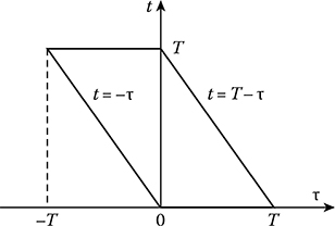
FIGURE 12.2 Integration domains.

The integration domain is shown in Figure 12.2. Changing the integration order, we obtain

$Var (E *) = \frac{2}{T} \int_{0}^{T} (1 - \frac{τ}{T}) R (τ) d τ . (12.116)$

If the interval of observation [0, T] is much more than the correlation interval τ_cor, we can change the upper integration limit in (12.116) by infinity and neglect the integrand term τ/T in comparison with unit. Then

$Var (E *) = \frac{2 Var (E_{E} | E_{0})}{T} \int_{0}^{\infty} R (τ) d τ . (12.117)$

If the normalized correlation function R (τ) is not a sign-changing function of the argument τ, the formula (12.117) takes a simple and obvious form:

$Var (E *) = \frac{2 Var (E_{E} | E_{0})}{T} τ_{cor} . (12.118)$

Consequently, if the ideal integrator integration time is sufficiently large in comparison with the correlation interval of stochastic process, then to determine the variance of mathematical expectation estimate of stochastic process there is a need to know only the values of variance and the ratio between the observation interval and correlation interval.

In the case of the sign-changing normalized correlation function with the argument τ, we can write

$\int_{0}^{T} | R (τ) | d τ > \int_{0}^{\infty} R (τ) d τ . (12.119)$

Thus, at T ≫ τ_cor the formula for the variance of the mathematical expectation estimate in the case of arbitrary correlation function of stationary stochastic process can be written in the following form:

$Var (E *) \leq \frac{2 Var (E_{E} | E_{0})}{T} τ_{cor} . (12.120)$

If T≫ τ_cor, the formula for the variance of the mathematical expectation estimate can be presented in the form using the spectral density S (co) of stochastic process that is related to the correlation function by the Fourier transform given by (12.25) and (12.27). In doing so, the formula for variance of the mathematical expectation estimate given by (12.117) takes the following form:

$Var (E *) \approx \frac{1}{T} \int_{- \infty}^{\infty} R (τ) d τ = \frac{1}{T} \int_{- \infty}^{\infty} S (ω) {\frac{1}{2 π} \int_{- \infty}^{\infty} \exp {j ω τ} d τ} d ω . (12.121)$

Taking into consideration that

$δ (ω) = \frac{1}{2 π} \int_{- \infty}^{\infty} \exp {j ω τ} d τ, (12.122)$

we obtain

$Var (E *) \approx {\frac{1}{T} S (ω) |}_{ω = 0} . (12.123)$

Thus, the variance of the mathematical expectation estimate of stochastic process is proportional to the spectral density value of fuctuation component of the considered stochastic process at co = 0 when the ideal integrator is used as a smoothing circuit. In other words, in the considered case, the variance of the mathematical expectation estimate of stochastic process is defined by spectral components about zero frequency. To obtain the current value of the mathematical expectation estimate and to investigate the realization of stochastic process within the limits of large interval of observation, we use the following estimate:

$E * (t) = \int_{0}^{T} h (τ) x (τ) d τ . (12.124)$

Evidently, this estimate has the same statistical characteristics as the estimate defined by (12.111).

In practice, the linear low-pass filters with constant parameters defined by the impulse response

$h (t) = {\begin{array}{l} h (t) & at & t \geq 0, \\ 0 & at & t < 0, \end{array} (12.125)$

are used as averaging devices. In this case, the formula describing the process at the low-pass filter output, taking into consideration the unbiasedness of estimate, takes the following form:

$E * (t) = c \int_{0}^{T} h (τ) x (T - τ) d τ, (12.126)$

where the constant factor c can be determined from the following condition:

$c = \frac{1}{\int_{0}^{T} h (τ) d τ} . (12.127)$

If a difference between the measurement instant and instant of appearance of stochastic process at the low-pass filter input is much more than the correlation interval τ_cor of the considered stochastic process and the low-pass filter time constant, then we can write

$E * (t) = \frac{\int_{0}^{\infty} h (t - τ) x (τ) d τ}{\int_{0}^{\infty} h (τ) d τ} . (12.128)$

The variance of the mathematical expectation estimate of stochastic process is defined as

$Var (E *) = c^{2} \int_{0}^{T} \int_{0}^{T} R (τ_{1} - τ_{2}) h (τ_{1}) h (τ_{2}) d τ_{1} d τ_{2} . (12.129)$

Introducing new variables τ₁ − τ₂ = τ and τ₂ = t and changing the order of integration, the formula for the variance of the mathematical expectation estimate can be presented in the following form:

$Var (E *) = 2 c^{2} \int_{0}^{T} R (τ) r_{h} (τ) d τ, (12.130)$

where, if T ≫ x_cor we can change the upper integration limit on infinity, and the introduced function

$r_{h} (τ) = \int_{0}^{T - τ} h (t) h (t + τ) d t, τ > 0, (12.131)$

corresponds to the correlation function of stochastic process forming at the output of filter with the impulse response h(t) when the “white” noise with the correlation function R(τ) = δ(τ) [8] excites the filter input.

When the process at the low-pass filter is stationary, that is, duration of exciting input stochastic process is much more in comparison with the low-pass filter constant time, the formula for the variance of the mathematical expectation estimate of stochastic process can be written in the following form:

$Var (E *) = \frac{1}{2 π} \int_{- \infty}^{\infty} S (ω) {| S (j ω) |}^{2} d ω, (12.132)$

using the spectral density

$S (j ω) = \int_{0}^{\infty} h (t) \exp {- j ω t} d t, (12.133)$

that is, the Fourier transform of the impulse response or frequency characteristic of the low-pass filter.

Consider an example where we compute the normalized variance of the mathematical expectation estimate Var(E*)/σ² as a function of the ratio T/τ_cor by averaging the investigated stochastic process by the ideal integrator with the pulse response given by (12.112) and RC-circuit, the impulse response of which takes the following form:

$h (t) = {\begin{array}{l} β \exp {- β τ} & at & 0 \leq t \leq T, \\ 0 & at & τ < 0, τ > T . \end{array} (12.134)$

The corresponding frequency characteristics take the following form:

$S (j ω) = \frac{1 - \exp {- j ω T}}{j ω T}; (12.135)$

$S (j ω) = \frac{β {1 - \exp {- (β + j ω) T}}}{β + j ω} . (12.136)$

As an example, consider the stationary stochastic process with the exponential correlation function given by (12.13) where the parameter α is inversely proportional to the correlation interval, that is,

$α = \frac{1}{τ_{cor}} . (12.137)$

Substituting (12.13) into (12.116) and (12.130), we obtain the normalized variance of the mathematical expectation estimate for the ideal integrator and RC filter:

$\frac{{Var}_{1} (E *)}{σ^{2}} = \frac{2}{p^{2}} [p - 1 + \exp {- p}]; (12.138)$

$\frac{{Var}_{1} (E *)}{σ^{2}} = λ \frac{1 - λ + 2 λ \exp {- p (1 + λ)} - (1 + λ) \exp {- 2 p λ}}{(1 - λ^{2}) {[1 - \exp {- λ p}]}^{2}}, (12.139)$

where

$p = α T = \frac{T}{τ_{cor}} and λ = \frac{β}{α} = \frac{τ_{cor}}{τ_{RC}} (12.140)$

are the ratio between the observation interval duration and the correlation interval and the ratio between the correlation interval and the RC filter time constant, respectively. The RC filter time constant τ_RC is defined as the correlation interval (see (12.21)).

If the observation time interval is large, that is, the condition λp ≫ 1 is satisfied, for example, for the RC filter, then the normalized variance of the mathematical expectation estimate will be limited by the RC filter, that is,

$\frac{{Var}_{2} (E *)}{σ^{2}} \approx \frac{λ}{1 + λ} . (12.141)$

At λ ≪ 1, that is, when the spectral bandwidth of considered stochastic process is much more than the averaging RC filter bandwidth, we can think that the RC filter plays the role of the ideal integrator and the estimate variance formula (12.139) under limiting transition, that is, λ → 0, takes a form given by (12.138).

Images

FIGURE 12.3 Normalized variance of the mathematical expectation estimate versus p at various values of λ.

Dependences of the normalized mathematical expectation estimate variances Var(E*)/σ².ver-sus the ratio p between the observation time interval and the correlation interval for the ideal integrator (the continuous line) and the RC filter (the dashed lines) are presented in Figure 12.3, where λ serves as the parameter. As we can see from Figure 12.3, in the case of the ideal inte-grator, the variance of estimate decreases proportionally to the increase in the observation time interval, but in the case of the RC filter, the variance of estimate is limited by the value given by (12.141). Taking into consideration λ ≪ 1, the normalized variance of the mathematical expectation estimate is limited by the value equal to the ratio between the correlation interval and the RC filter time constant in the limiting case.

It is worthwhile to compare the mathematical expectation estimate using the ideal integrator with the optimal estimate, the variance of which Var(E_E) is given by (12.48). Relative increase in the variance using the ideal integrator in comparison with the optimal estimate is defined as

$κ = \frac{{Var}_{1} (E *) - Var (E_{E})}{Var (E_{E})} = \frac{(2 + p) [p - 1 + \exp {- p}]}{p^{2}} - 1. (12.142)$

Images

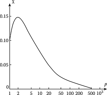
FIGURE 12.4 Relative increases in variance as a function of T/τ_cor.

Relative increase in the variance as a function of T/τ_cor is shown in Figure 12.4. As we can see from Figure 12.4, the relative increase in the variance of the mathematical expectation estimate of stochastic process possessing the correlation function given by (12.13) using the ideal integrator is less than 0.01, in comparison with the optimal estimate. At the same time, the maximum relative increase in the variance is 0.14 and corresponds to p≈ 2.7. This maximum increase is caused by a rapid decrease in the optimal estimate variance in comparison with the estimate obtained by the ideal integrator at small values of the observation time interval. However, as p → ∞, both estimates are equivalent, as it was expected.

Consider the normalized variances of the mathematical expectation estimates of stochastic process using the ideal integrator for the following normalized correlation functions that are widely used in practice. We analyze two RCfilters connected in series and the “white” noise excites the input of this linear system. In this case, the normalized correlation function takes the following form:

$R (τ) = (1 + α | τ |) \exp {- α | τ |}, α = \frac{1}{R C} . (12.143)$

In doing so, the normalized variance of the mathematical expectation estimate of stochastic process is defined as

$\frac{{Var}_{3} (E *)}{σ} = \frac{2 [2 p_{1} - 3 + (3 + p_{1}) \exp {- p_{1}}]}{p_{1}^{2}}, (12.144)$

where

$p_{1} = α T = \frac{2 T}{τ_{cor}} and τ_{cor} = \frac{2}{α} . (12.145)$

The set of considered stochastic processes has the normalized correlation functions that are approx-imated in the following form:

$R (τ) = \exp {- α | τ |} \cos ϖ τ . (12.146)$

Depending on the relationships between the parameters α and ϖ, the normalized correlation function (12.146) describes both the low-frequency (α ≫ ϖ) and high-frequency (α ≪ ϖ) stochastic processes. The normalized variance of the mathematical expectation estimate of stochastic process with the normalized correlation function given by (12.146) takes the following form:

$\frac{{Var}_{4} (E *)}{σ^{2}} = \frac{2 [p_{1} (1 + η^{2}) - (1 - η^{2})] + 2 \exp {- p_{1}} [(1 - η^{2}) \cos p_{1} η - 2 η \sin p_{1} η]}{p_{1}^{2} {(1 + η^{2})}^{2}}, (12.147)$

where η = ϖα^ϖ1. At ϖ = 0 (η = 0) in (12.147), as in the particular case, we obtain (12.138); that is, we obtain the normalized variance of the mathematical expectation estimate of stochastic process with the exponential correlation function given by (12.13) under integration using the ideal integrator. In this case, (12.147) is essentially simplified at ϖ = α:

$\frac{{Var}_{4} (E *)}{σ^{2}} = \frac{p_{1} - \exp {- p_{1}} \sin p_{1}}{p_{1}^{2}}, at ϖ = α . (12.148)$

Images

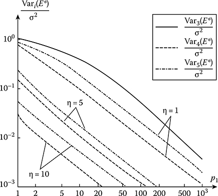
FIGURE 12.5 Normalized variances given by (12.144), (12.147), and (12.149) as functions of p₁ with the parameter η.

As applied to the correlation function given by (12.14), the normalized variance of the mathematical expectation estimate of stochastic process is defined by

$\frac{{Var}_{5} (E *)}{σ^{2}} = \frac{2 [2 p_{1} (1 + η_{1}^{2}) - (3 - η_{1}^{2})] + 2 \exp {- p_{1}} [(3 - η_{1}^{2}) \cos p_{1} η_{1} - 3 η_{1} + η_{1}^{- 1} \sin (p_{1} η_{1})]}{p_{1}^{2} {(1 + η_{1}^{2})}^{2}}, (12.149)$

where η₁ = ϖ₁α⁻¹. As ϖ₁ → 0 η₁ → 0), the correlation function given by (12.14) can be written as the correlation function given by (12.143), and the formula (12.149) is changed to (12.144).

The normalized variances of the mathematical expectation estimate of stochastic process given by (12.144), (12.147), and (12.149) as a function of the parameter p₁ with the parameter r), are shown in Figure 12.5. As expected, at the same value of the parameter p₁, the normalized variance of the mathematical expectation estimate of stochastic process decreases corresponding to an increase r) characterizing the presence of quasiharmonical components in the considered stochastic process.

Discussed procedures to measure the mathematical expectation assume that there are no limitations of instantaneous values of the considered stochastic process in the course of measurement. Presence of limitations leads to additional errors while measuring the mathematical expectation of stochastic process.

Determine the bias and variance of estimate applied both to the symmetrical inertialess signal limiter (see Figure 12.6) and to the asymmetrical inertialess signal limiter (see Figure 12.7) when the input of the signal limiter is excited by the Rayleigh stochastic process. In doing so, we assume that the mathematical expectation is defined according to (12.113) where we use y(t) = g[x(t)] instead of x(t) and g(x) as the characteristic functions of transformation. The variance of the mathematical expectation estimate of stochastic process is defined by (12.116) where under the correlation function R(x) we should understand the correlation function R_y(τ) defined as

$R_{y} (τ) = \int_{- \infty}^{\infty} \int_{- \infty}^{\infty} g (x_{1}) g (x_{2}) p_{2} (x_{1}, x_{2}; τ) d x_{1} d x_{2} - E_{y}^{2} . (12.150)$

Images

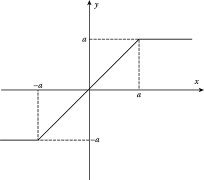
FIGURE 12.6 Symmetric inertialess signal limiter performance.

Images

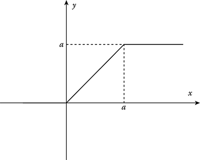
FIGURE 12.7 Asymmetric inertialess signal limiter performance.

Let the Gaussian stochastic process excite the input of nonlinear device (Figure 12.6) and the trans-formation be described by the following function:

$y = g (x) = {\begin{array}{l} a & if & x > a, \\ x & if & - a \leq x \leq a, \\ - a & if & x < - a . \end{array} (12.151)$

The bias of estimate is defined as

$b (E *) = \int_{- \infty}^{\infty} g (x) p (x) d x - E_{0} = - a \int_{- \infty}^{- a} p (x) d x + \int_{- a}^{a} x p (x) d x + a \int_{a}^{\infty} p (x) d x - E_{0} . (12.152)$

Substituting the one-dimensional pdf of Gaussian stochastic process

$p (x) = \frac{1}{\sqrt{2 π Var (x)}} \exp {- \frac{{(x - E_{0})}^{2}}{2 Var (x)}} (12.153)$

into (12.152), we obtain the bias of the mathematical expectation estimate of stochastic process in the following form:

$b (E *) = \sqrt{Var (x)} {χ [Q (χ - q) - Q (χ + q)] - q [Q (χ + q) + Q (χ - q)] - + \frac{1}{\sqrt{2 π}} {\exp [- 0.5 {(χ + q)}^{2}] - \exp [- 0.5 {(χ - q)}^{2}]}}, (12.154)$

where

$χ = \frac{α}{\sqrt{Var (x_{0})}} and q = \frac{E_{0}}{\sqrt{Var (x_{0})}} (12.155)$

are the ratio of the limitation threshold and the mathematical expectation for the square root of the variance of the observed realization of stochastic process; Q(x) is the Gaussian Q function given by (12.68).

To determine the variance of mathematical expectation estimate of stochastic process according to (12.116) and (12.150), there is a need to expand the two-dimensional pdf of Gaussian stochastic process in series [9]

$p_{2} (x_{1}, x_{2}; τ) = \frac{1}{Var (x)} \sum_{v = 0}^{\infty} Q^{(v + 1)} (\frac{x_{1} - E_{0}}{\sqrt{Var (x)}}) Q^{(v + 1)} (\frac{x_{2} - E_{0}}{\sqrt{Var (x)}}) \frac{ℛ^{v} (τ)}{v!}, (12.156)$

where ℛ(τ) is the normalized correlation function of the initial stochastic process ξ(t);

$Q^{(v + 1)} (z) = \frac{d^{v}}{d z^{v}} [\frac{\exp {- 0.5 z^{2}}}{\sqrt{2 π}}], v = 0, 1, 2, \dots . (12.157)$

are the derivatives of (v + 1)th order of the Gaussian Q function.

Substituting (12.156) into (12.150) and (12.1167) and taking into consideration that

$E_{y} = \frac{1}{σ^{2}} \int_{- \infty}^{\infty} g (x) Q' (\frac{x - E_{0}}{σ}) d x, (12.158)$

we obtain

$Var (E *) = \frac{1}{σ^{2}} \sum_{v = 1}^{\infty} \frac{1}{v!} {\int_{- \infty}^{\infty} g (x) Q^{(v + 1)} (\frac{x - E_{0}}{σ}) d x}^{2} \frac{2}{T} \int_{0}^{T} (1 - \frac{τ}{T}) ℛ^{v} (τ) d τ . (12.159)$

Computing the integral in the braces, we obtain

$Var (E *) = σ^{2} \sum_{v = 1}^{\infty} \frac{1}{v!} {[Q^{(v - 1)} (χ - q) - Q^{(v - 1)} (- χ - q)]}^{2} \frac{2}{T} \int_{0}^{T} (1 - \frac{τ}{T}) ℛ^{v} (τ) d τ . (12.160)$

As χ → ∞, the derivatives of the Gaussian Q function tend to approach zero. As a result, only the term at ν = 1 remains and we obtain the initial formula (12.116).

In practical applications, the stochastic process measurements are carried out, as a rule, under the conditions of “weak” limitations of instantaneous values, that is, under the condition (χ − |q|) ≥ 1.5 ÷ 2. In this case, the first term at ν = 1 in (12.160) plays a very important role:

$Var (E *) \approx {[1 - Q (χ - q) - Q (χ + q)]}^{2} \frac{2 σ^{2}}{T} \int_{0}^{T} (1 - \frac{τ}{T}) ℛ (τ) d τ, (12.161)$

where, at sufficiently high values, that is, (χ − q) ≥ 3, the term in square brackets is very close to unit and we may use (12.116) to determine the variance of mathematical expectation estimate of stochastic process.

In practice, the Rayleigh stochastic processes are widely employed because this type of stochastic processes have a wide range of applications. In particular, the envelope of narrow-band Gaussian stochastic process described by the Rayleigh pdf can be presented in the following form:

$z (t) = x (t) \cos [2 π f_{0} t + φ (t)], (12.162)$

where

x(t) is the envelope
φ(t) is the phase of stochastic process

Representation in (12.162) assumes that the spectral density of narrow-band stochastic process is concentrated within the limits of narrow bandwidth Δf.with the central frequency f₀ and the condition f₀ ≫ Δf. As applied to the symmetrical spectral density, the correlation function of stationary narrow-band stochastic process takes the following form:

$R_{z} (τ) = σ^{2} ℛ (τ) \cos (2 π f_{0} τ) . (12.163)$

In doing so, the one-dimensional Rayleigh pdf can be written as

$f (x) = \frac{x}{σ^{2}} \exp {- \frac{x^{2}}{2 σ^{2}}}, x \geq 0. (12.164)$

The first and second initial moments and the normalized correlation function of the Rayleigh stochastic process can be presented in the following form:

${\begin{array}{l} 〈 ξ (t) 〉 = \sqrt{\frac{π}{2} σ^{2},} \\ 〈 ξ^{2} (t) 〉 = 2 σ^{2}, \\ ρ (τ) \approx ℛ^{2} (τ) . \end{array} (12.165)$

As applied to the Rayleigh stochastic process and nonlinear transformation (see Figure 12.7) given as

$y = g (x) = {\begin{array}{l} a & if & x > a, \\ x & if & 0 \leq x \leq a, \end{array} (12.166)$

the bias of the mathematical expectation estimate takes the following form:

$b (E *) = E_{y} - E_{0} = \int_{0}^{\infty} g (x) f (x) d x - E_{0} = \sqrt{2 π σ^{2}} Q (χ), (12.167)$

where χ is given by (12.155). As χ → ∞, the mathematical expectation estimate, as it would be expected, is unbiased.

Determining the variance of mathematical expectation estimate of stochastic process in accordance with (12.116) and (12.150) is very difficult in the case of Rayleigh stochastic process. It is evident that to determine the variance of mathematical expectation estimate of stochastic process in the first approximation, the formula (12.116) has to be true, provided the condition χ ≥ 2–3 is satisfied, which is analogous to the Gaussian stochastic process at weak limitation.

12.5 Estimate of Mathematical Expectation at Stochastic Process Sampling

In practice, we use digital measuring devices to measure the parameters of stochastic processes after sampling. Naturally, we do not use a part of information that is outside a sample of stochastic process.

Let the Gaussian stochastic process χ(t) be observed at some discrete instants t_i. Then, there are a set of samples x_i = x(t), i = 1, 2,…, N at the input of digital measuring device. As a rule, a sample clamping of the observed stochastic process is carried out over equal time intervals Δ = t_i+1 − t_i. Each sample value can be presented in the following form:

$x_{i} = E_{i} + x_{0_{i}} = E s_{i} + x_{0_{i}} (12.168)$

as in (12.2), where E_i = E s_i = Es(t_i) is the mathematical expectation and x_{0_i} = x₀ (t_i) is the realization of the centralized Gaussian stochastic process at the instant t = t_i. A set of samples x_i are characterized by the conditional N-dimensional pdf

$f_{N} (x_{1}, \dots, x_{N} | E) = \frac{1}{{(2 π)}^{- 0.5 N} \sqrt{\det ‖ R_{i j} ‖}} \exp {- 0.5 \sum_{i = 1}^{N} \sum_{j = 1}^{N} (x_{i} - E_{i}) (x_{j} - E_{j}) C_{i j}}, (12.169)$

where

det ||R_ij|| is the determinant of the correlation matrix ||R_ij|| = R of the N × N order
C_ij is the elements of the matrix ||C_ij|| = C, which is the reciprocal matrix with respect to the correlation matrix and the elements C_ij are defined from the following equation:

$\sum_{l = 1}^{N} C_{i j} R_{i j} = δ_{i j} = {\begin{array}{l} 1 & if & i = j, \\ 0 & if & i \neq j . \end{array} (12.170)$

The conditional multidimensional pdf in (12.169) is the multidimensional likelihood function of the parameter E of stochastic process. Solving the likelihood equation with respect to the parameter E, we obtain the formula for the mathematical expectation estimate of stochastic process:

$E_{E} = \frac{\sum_{i = 1, j = 1}^{N} x_{i} s_{j} C_{i j}}{\sum_{i = 1, j = 1}^{N} s_{i} s_{j} C_{i j}} . (12.171)$

This formula can be written in a simple form if we introduce the weight coefficients

$υ_{i} = \sum_{j = 1}^{N} s_{j} C_{i j}, (12.172)$

which satisfy, as the function υ(t) given by (12.7), the system of equations

$\sum_{l = 1}^{N} R_{i l} υ_{l} = s_{i}, i = 1, 2, \dots, N . (12.173)$

In doing so, the mathematical expectation estimate can be presented in the following form:

$E_{E} = \frac{\sum_{i = 1}^{N} x_{i} υ_{i}}{\sum_{i = 1}^{N} s_{i} υ_{i}} . (12.174)$

The mathematical expectation of estimate takes the following form:

$〈 E_{E} 〉 = \frac{\sum_{i = 1}^{N} 〈 x_{i} 〉 υ_{i}}{\sum_{i = 1}^{N} s_{i} υ_{i}} = E_{0} . (12.175)$

The variance of estimate in accordance with (12.172) can be presented in the following form:

$Var (E_{E}) = \frac{\sum_{i = 1, j = 1}^{N} R_{i j} υ_{i} υ_{j}}{{[\sum_{i = 1}^{N} s_{i} υ_{i}]}^{2}} = \frac{1}{\sum_{i = 1}^{N} s_{i} υ_{i}} . (12.176)$

The weight coefficients are determined using a set of linear equations:

${\begin{array}{l} σ^{2} υ_{1} + R_{1} υ_{2} + R_{2} υ_{3} + \dots + R_{N - 1} υ_{N} = s_{1}, \\ R_{1} υ_{1} + σ^{2} υ_{2} + R_{1} υ_{3} + \dots + R_{N - 2} υ_{N} = s_{2}, \\ ⋮ ⋮ \\ R_{N - 1} υ_{1} + R_{N - 2} υ_{2} + R_{N - 3} υ_{3} + \dots + σ^{2} υ_{N} = s_{N}, \end{array} (12.177)$

where R_l = R (lΔ) are the elements of the correlation matrix of difference in time |i − j|Δ = lΔ, l = 0, 1,…, N − 1. The solution derived from this system of linear equations can be presented in the following form:

$υ_{j} = \frac{\det ‖ G_{i j} ‖}{\det ‖ R_{i j} ‖}, j = 1, 2, \dots, N, (12.178)$

where det ||G_ij|| is the determinant of matrix obtained from the matrix ||R_ij|| = R by substituting the column containing elements s₁, s₂,…, s_N instead of the jth column. In the case of independent samples of stochastic process, that is, R_ij = 0 at i ≠ j and R_ii = σ², the correlation matrix and its recip-rocal matrix will be diagonal. In doing so, for all i = 1, 2,…, N the weight coefficients are defined as

$υ_{i} = \frac{s_{i}}{σ^{2}} . (12.179)$

Substituting (12.179) into (12.174) and (12.176) we obtain

$E_{E} = \frac{\sum_{i = 1}^{N} x_{i} s_{i}}{\sum_{i = 1}^{N} s_{i}^{2}}, (12.180)$

$Var (E_{E}) = \frac{σ^{2}}{\sum_{i = 1}^{N} s_{i}^{2}} . (12.181)$

If the observed stochastic process is stationary, that is, s_i = 1 ∀i, i = 1, 2,…, N, even in the presence of independent samples, we obtain the mean and variance of the mean

$E * = \frac{1}{N} \sum_{i = 1}^{N} x_{i}; (12.182)$

$Var (E *) = \frac{σ^{2}}{N}, (12.183)$

respectively.

Now, consider the estimate of stationary stochastic process mathematical expectation with the correlation function given by (12.13). Denote ψ = exp{−αΔ}. In this case, the correlation matrix takes the following form:

$‖ R_{i j} ‖ = σ^{2 N} [\begin{array}{l} 1 & ψ & ψ^{2} & \dots & ψ^{N - 1} \\ ψ & 1 & ψ & \dots & ψ^{N - 2} \\ ψ^{2} & ψ & 1 & \dots & ψ^{N - 3} \\ ⋮ & ⋮ \\ ψ^{N - 1} & ψ^{N - 2} & ψ^{N - 3} & \dots & 1 \end{array}] . (12.184)$

The determinant of this matrix and its reciprocal matrix are defined in the following form [10]:

$\det ‖ R_{i j} ‖ = σ^{2 N} {(1 - ψ^{2})}^{N - 1}, (12.185)$

$‖ C_{i j} ‖ = \frac{1}{(1 - ψ^{2}) σ^{2}} [\begin{array}{l} 1 & - ψ & 0 & \dots & 0 \\ - ψ & 1 + ψ^{2} & - ψ & \dots & 0 \\ 0 & - ψ & 1 + ψ^{2} & \dots & 0 \\ ⋮ & ⋮ \\ 0 & 0 & 0 & \dots & 1 \end{array}] . (12.186)$

It is important to note that all elements of the reciprocal matrix are equal to zero, except for the elements of the main diagonal and the elements flanking the main diagonal from right and left. As we can see from (12.172) and (12.186), the optimal values of weight coefficients are defined as

${\begin{matrix} υ_{1} & = υ_{N} = \frac{1}{(1 + ψ) σ^{2}}; \\ υ_{2} & = υ_{3} = \dots = υ_{N - 1} = \frac{1 - ψ}{(1 + ψ) σ^{2}} . \end{matrix} (12.187)$

Substituting the obtained weight coefficients into (12.174) and (12.176), we have

$E_{E} = \frac{(x_{1} + x_{N}) + (1 - ψ) \sum_{i = 2}^{N - 1} x_{i}}{N - (N - 2) ψ}; (12.188)$

$Var (E_{E}) = σ^{2} \frac{1 + ψ}{N - (N - 2) ψ} . (12.189)$

Dependence of the normalized variance of the optimal mathematical expectation estimate versus the values ψ of the normalized correlation function between the samples and the various numbers of samples N is shown in Figure 12.8. As we can see from Figure 12.8, starting from ψ ≥ 0.5, the variance of estimation increases rapidly corresponding to an increase in the value of the normalized correlation function, which tends to approach the variance of the observed stochastic process as ψ → 1.

We can obtain the formulae (12.188) and (12.189) by another way without using the maximum likelihood method. For this purpose, we suppose that

$E * = \sum_{i = 1}^{N} x_{i} h_{i} (12.190)$

Images

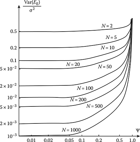
FIGURE 12.8 Normalized variance of the optimal mathematical expectation estimate versus ψ and the number of samples N.

can be used as the estimate, where h_i are the weight coefficients satisfying the following condition

$\sum_{i = 1}^{N} h_{i} = 1 (12.191)$

for the unbiased estimations. The weight coefficients are chosen from the condition of minimization of the variance of mathematical expectation estimate. As applied to observation of stationary stochastic process possessing the correlation function given by (12.13), the weight coefficients h_i are defined in Ref. [11] and related with the obtained weight coefficients (12.187) by the following relationship:

$h_{i} = \frac{υ_{i}}{\sum_{i = 1}^{N} υ_{i}} . (12.192)$

In the limiting case, as Δ → 0 the formulae in (12.188) and (12.189) are changed into (12.48) and (12.49), respectively. Actually, as Δ → 0 and if (n − 1) Δ = T = const and exp{−αΔ} ≈ 1 − αΔ, the summation in (12.188) is changed by integration and x₁ and x_N are changed in x (0) and x (T), respectively. In practice, the equidistributed estimate (the mean) given by (12.182) is widely used as the mathematical expectation estimate of stationary stochastic process that corresponds to the constant weight coefficients h_i ≈ N⁻¹, i = 1, 2,…, N given by (12.190).

Determine the variance of the mathematical expectation estimate assuming that the samples are equidistant from each other on the value Δ. The variance of the mathematical expectation estimate of stochastic process is defined as

$Var (E *) = \frac{1}{N^{2}} \sum_{i = 1, j = 1}^{N} R (t_{1} - t_{j}) = \frac{1}{N^{2}} \sum_{i = 1, j = 1}^{N} R [(i - j) Δ] . (12.193)$

Images

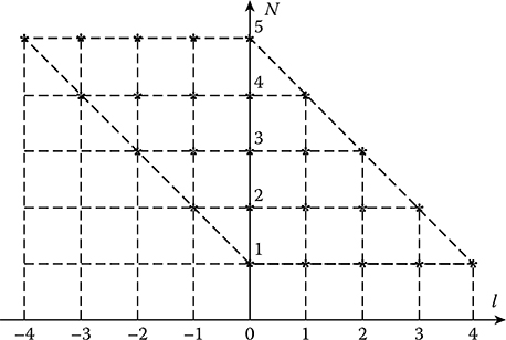
FIGURE 12.9 Domain of indices.

The double summation in (12.193) can be changed in a more convenient form. For this purpose, there is a need to change indices, namely, l = i − j and j = j, and change the summation order in the domain shown in Figure 12.9. In this case, we can write

$Var (E *) = \frac{1}{N^{2}} \sum_{j = 1}^{N} \sum_{l = - j}^{N - j} ℛ (l Δ) = \frac{1}{N^{2}} {N σ^{2} + 2 \sum_{i = 1}^{N - 1} (N - i) ℛ (i Δ)} = \frac{σ^{2}}{N} {1 + 2 \sum_{i = 1}^{N - 1} (1 - \frac{i}{N}) ℛ (i Δ)}, (12.194)$

where ℛ(iΔ) is the normalized correlation function of observed stochastic process. As we can see from (12.194), if the samples are not correlated the formula (12.183) can be considered as a particular case.

If the correlation function of observed stochastic process is described by (12.13), the variance of the equidistributed estimate of mathematical expectation is defined as

$Var (E *) = σ^{2} \frac{N (1 - ψ^{2}) + 2 ψ (ψ^{N} - 1)}{N^{2} {(1 - ψ)}^{2}}, (12.195)$

where, as before, ψ = exp{−αΔ}. We have just obtained (12.195) by taking into consideration the formula for summation [12]

$\sum_{i = 0}^{N - 1} (a + i r) q^{i} = \frac{a - [a + (N - 1) r] q^{N}}{1 - q} + \frac{r q (1 - q^{N - 1})}{1 - q^{2}} . (12.196)$

Computations made by the formula (12.195) show that the variance of the equidistributed estimate of mathematical expectation differs from the variance of the optimal estimate (12.189). Figure 12.10. represents a relative increase in the variance of the equidistributed estimate of mathematical expec-tation in comparison with the variance of the optimal estimate

$ε = \frac{Var (E *) - Var (E_{E})}{Var (E_{E})} (12.197)$

Images

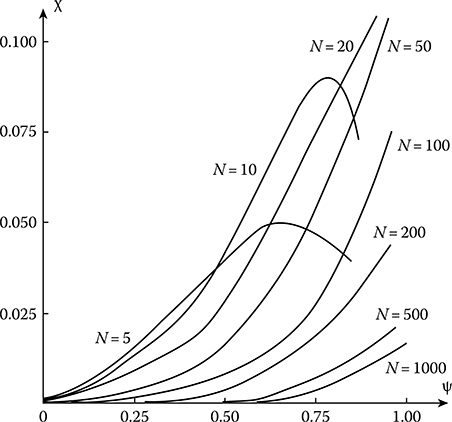
FIGURE 12.10 Relative increase in the variance of equidistributed estimate of mathematical expectation as a function of the normalized correlation function between samples.

as a function of values of the normalized correlation function between the samples ψ for various numbers of samples. Naturally, if the relative increase in the variance is low, then the magnitude of the normalized correlation function between samples will be low as well. Similar to the mathematical expectation estimate by the continuous realization of stochastic process, the presence of maxima is explained by the fact that in the case of small numbers of samples N and sufficiently large magnitude ψ, the variance of the optimal estimate decreases rapidly in comparison with the variance of the equidistributed estimate of mathematical expectation. As we can see from Figure 12.10, the magnitude of the normalized correlation function between samples is less than ψ = 0.5, then the optimal and equidistributed estimates coincide practically.

As applied to the normalized correlation function (12.146), the normalized variance of estimate is defined as

$\frac{Var (E *)}{σ^{2}} = \frac{N (1 - ψ^{2}) [1 + ψ^{2} - 2 ψ \cos (Δ ϖ)] + 2 ψ^{(2 N + 1)} {\cos [(N + 1) Δ ϖ] - 2 ψ \cos (N Δ ϖ) + ψ^{2} \cos [(N - 1) Δ ϖ]}}{N^{2} {[1 + ψ^{2} - 2 ψ \cos (Δ ϖ)]}^{2}} - \frac{2 ψ^{2} [(1 + ψ^{2}) \cos (Δ ϖ) - 2 ψ]}{N^{2} {[1 + ψ^{2} - 2 ψ \cos (Δ ϖ)]}^{2}}, (12.198)$

where, as before, ψ = exp{−αΔ}. At ϖ = 0, we obtain the formula (12.195). In the case of large numbers of samples, the formula (12.198) is simplified

$\frac{Var (E *)}{σ^{2}} \approx \frac{(1 - ψ^{2})}{N [1 + ψ^{2} - 2 ψ \cos (Δ ϖ)]}, N Δ α ≫ 1. (12.199)$

As we can see from (12.199), in the case of stochastic process with the correlation function given by (12.146) the equidistributed estimate may possess the estimate variance that is less than the variance of estimate by the same number of the uncorrelated samples. Actually, if the samples are taken over the interval

$Δ = \frac{π + 2 π k}{ϖ}, k = 0, 1, \dots, (12.200)$

then the minimal magnitude of the normalized variance of estimate can be presented in the following form:

${\frac{Var (E *)}{σ^{2}} |}_{\min} \approx \frac{1}{N} \times \frac{1 - ψ}{1 + ψ}, N Δ α ≫ 1. (12.201)$

Otherwise, if the interval between samples is chosen such that

$Δ = \frac{2 π k}{ϖ}, k = 0, 1, \dots . (12.202)$

then the maximum value of the normalized variance of estimate takes the following form:

${\frac{Var (E *)}{σ^{2}} |}_{\max} \approx \frac{1}{N} \times \frac{1 + ψ}{1 - ψ} . (12.203)$

Thus, for some types of correlation functions, the variance of the equidistributed estimate of mathematical expectation by the correlated samples can be lesser than the variance of estimate by the same numbers of uncorrelated samples.

If the interval between samples Δ is taken without paying attention to the conditions discussed previously, then the value Δϖ = φ can be considered as the random variable with the uniform distribution within the limits of the interval [0, 2π]. Averaging (12.199) with respect to the random variable φ uniformly distributed within the limits of the interval [0, 2π], we obtain the variance of the mathematical expectation estimate of stochastic process by N uncorrelated samples

${\frac{Var (E *)}{σ^{2}}}_{φ} = \frac{1 - ψ^{2}}{N} \int_{0}^{2 π} \frac{d φ}{1 + ψ^{2} - 2 ψ \cos φ} = \frac{1}{N} . (12.204)$

Of definite interest for the definition of the mathematical expectation estimate is the method to measure the stochastic process parameters by additional signals [13, 14]. In this case, the realization x(t_i) = x_i of the observed stochastic process ξ(t_i) = ξ_i is compared with the realization v(t_i) = v_i of the additional stochastic process ζ(t_i) = ζ_i. A distinct feature of this measurement method is that the values x_i of the observed stochastic process realization must be with the high probability within the limits of the interval of possible values of the additional stochastic process. Usually, it is assumed that the values of the additional stochastic process are independent from each other and from the values of the observed stochastic process.

To further simplify an analysis of the stochastic process parameters and the definition of the mathematical expectation, we believe that the values x_i are independent of each other and the random variables ζ_i are uniformly distributed within the limits of the interval [−A, A], that is,

$f (v) = \frac{1}{2 A}, - A \leq v \leq A . (12.205)$

As applied to the pdf given by (12.203), the following condition must be satisfied

$P [- A \leq ξ \leq A] \approx 1 (12.206)$

in the case of the considered method to measure the stochastic process parameters. As a result of comparison, a new independent random variable sequence ς_i is formed:

$ς_{i} = x_{i} - v_{i} . (12.207)$

The random variable sequence ς_i can be transformed to the new independent random variable sequence η_i by the nonlinear inertialess transformation g(ε)

$η_{i} = g (ε_{i}) = sgn [ς_{i} = ξ_{i} - ζ_{i}] = {\begin{array}{l} 1, & ξ_{i} \geq ζ_{i}, \\ - 1, & ξ < ζ_{i} . \end{array} (12.208)$

Determine the mathematical expectation of random variable η_i under the condition that the random variable ξ_i takes the fixed value x and the following condition |x| ≤ A is satisfied:

$〈 (η_{i} | x) 〉 = 1 \times P (v < x) - 1 \times P (v > x) = 2 \times P (v < x) - 1 = \frac{x}{A} . (12.209)$

The unconditional mathematical expectation of the random variable η_i can be presented in the following form:

$〈 η_{i} 〉 = \int_{- A}^{A} 〈 (η_{i} | x) 〉 p (x) d x \approx \frac{1}{A} \int_{- \infty}^{\infty} x p (x) d x = \frac{E_{0}}{A} . (12.210)$

Based on the obtained representation, we can consider the following value

$\tilde{E} = \frac{A}{N} \sum_{i = 1}^{N} y_{i}, (12.211)$

as the mathematical expectation estimate of random variable, where y_i is the sample of random sequence η_i. At that point, it is not difficult to see that the considered mathematical expectation estimate is unbiased for the accepted conditions. The structural diagram of device measuring the mathematical expectation using the additional signals is shown in Figure 12.11. The counter defines a difference between the positive and negative pulses forming at the transformer output g(ε).The functional purpose of other elements is clear from the diagram.

Images

FIGURE 12.11 Measurer of mathematical expectation.

If we take into consideration the condition that P(x < −A) ≠ 0 and P(x > A) ≠ 0, then the mathematical expectation estimate given by (12.211) has a bias defined as

$b (\tilde{E}) = \tilde{E} - E_{0} = - {\int_{- \infty}^{- A} x p (x) d x + \int_{A}^{\infty} x p (x) d x} . (12.212)$

The variance of the mathematical expectation given by (12.211) can be presented in the following form:

$Var (\tilde{E}) = \frac{A^{2}}{N^{2}} \sum_{i = 1, j = 1}^{N} 〈 y_{i} y_{j} 〉 - E_{0}^{2} . (12.213)$

Taking into consideration the statistical independence of the samples y_i, we have

$〈 y_{i} y_{j} 〉 = {\begin{array}{l} 〈 y_{i}^{2} 〉, & i = j, \\ 〈 y_{i} 〉 〈 y_{j} 〉, & i \neq j . \end{array} (12.214)$

According to (12.208),

$〈 η_{i}^{2} 〉 = 〈 {(η_{i} | x)}^{2} 〉 = η_{i}^{2} = y_{i}^{2} = 1. (12.215)$

Consequently, the variance of the mathematical expectation estimate is simplified and takes the following form:

$Var (\tilde{E}) = \frac{A^{2}}{N} (1 - \frac{E_{0}^{2}}{A^{2}}) . (12.216)$

As we can see from (12.216), since $E_{0}^{2} < A^{2}$ , the variance of the mathematical expectation of stochastic process is defined completely by half-interval of possible values of the additional random sequence.

Comparing the variance of the mathematical expectation estimate given by (12.216) with the variance of the mathematical expectation estimate by N independent samples given by (12.183)

$\frac{Var (\tilde{E})}{Var (E *)} = \frac{A^{2}}{σ^{2}} (1 - \frac{E_{0}^{2}}{A^{2}}), (12.217)$

we see that the considered procedure to estimate the mathematical expectation possesses the high variance since A² > σ² and $E_{0}^{2} < A^{2}$ .

If we know a priori that the observed stochastic sequence v(t_i) = v_i is a positive value, then we can use the following pdf:

$\begin{matrix} p (v) = \frac{1}{A}, & 0 \leq v \leq A \end{matrix}, (12.218)$

and the following function:

$η_{i} = g (ε_{i}) = {\begin{array}{l} 1, & ξ_{i} \geq ζ_{i}, \\ 0, & ξ < ζ_{i} \end{array} (12.219)$

as the nonlinear transformation η = g(ε). In doing so, the following condition must be satisfied:

$P [0 \leq ξ \leq A] \approx 1. (12.220)$

As we can see from (12.220), this condition is analogous to the condition given by (12.206).

The conditional mathematical expectation of random variable η_i at ξ_i = x takes the following form:

$〈 (η_{i} | | x |) 〉 = 1 \times P (v < x) + 0 \times P (v > x) = \int_{0}^{x} p (v) d v = \frac{x}{A} . (12.221)$

In doing so, the unconditional mathematical expectation of the random variable η_i is defined in the following form:

$〈 η_{i} 〉 \approx \frac{1}{A} \int_{0}^{\infty} x p (x) d x = \frac{E_{0}}{A} . (12.222)$

For this reason, if the mathematical expectation estimate of the random sequence ξ_i is defined by (12.211) it will be unbiased at the first approximation.

The variance of the mathematical expectation estimate, as we discussed previously, is given by (12.213). In doing so, the conditional second moment of the random variable η_i is determined analogously as shown in (12.221):

$〈 {(η_{i} | x)}^{2} 〉 = \int_{0}^{x} p (v) d v = \frac{x}{A} . (12.223)$

The unconditional moment is given by

$〈 η_{i}^{2} 〉 = 〈 y_{i}^{2} 〉 = \int_{0}^{\infty} 〈 {(η_{i} | x)}^{2} 〉 p (x) d x = \frac{E_{0}}{A} . (12.224)$

Taking into consideration (12.223) and (12.224) under definition of the variance of the mathematical expectation estimate, we have

$Var (\tilde{E}) = \frac{A E_{0}}{N} (1 - \frac{E_{0}}{A}) . (12.225)$

Thus, in the considered case, the variance of the mathematical expectation estimate is defined by the interval of possible values of the additional stochastic sequence and is independent of the variance of the observed stochastic process and is forever more than the variance of the equidistributed estimate of the mathematical expectation by independent samples. For example, if the observed stochastic sequence subjected to the uniform pdf coinciding in the limiting case with (12.218), then the variance of the mathematical expectation for the considered procedure is defined as

$Var (\tilde{E}) = \frac{A^{2}}{4 N} (12.226)$

and the variance of the mathematical expectation in the case of equidistributed estimate of the mathematical expectation is given by

$Var (E *) = \frac{A^{2}}{12 N}; (12.227)$

that is, the variance of the mathematical expectation estimate is three times more than the variance of the mathematical expectation in the case of equidistributed estimate of the mathematical expectation under the use of additional stochastic signals in the considered limiting case when the observed and additional random sequences are subjected to the uniform pdf. At other conditions, a difference in variances of the mathematical expectation estimate is higher.

As applied to (12.219), the flowchart of the mathematical expectation measurer using additional stochastic signals shown in Figure 12.11 is the same, but the counter defines the positive pulses only in accordance with (12.219).

12.6 Mathematical Expectation Estimate Under Stochastic Process Amplitude Quantization

Define an effect of stochastic process quantization by amplitude on the estimate of its mathematical expectation. With all this going on, we assume that a quantization can be considered as the inertia-less nonlinear transformation with the constant quantization step and the number of quantization levels is so high that the quantized stochastic process cannot be outside the limits of staircase characteristic of the transform g(x), the approximate form of which is shown in Figure 12.12. The pdf p(x) of observed stochastic process possessing the mathematical expectation that does not match with the middle between the quantization thresholds x_i and x_i+1 is presented in Figure 12.12.

Transformation or quantization characteristic y = g(x) can be presented in the form of summation of the rectangular functions shown in Figure 12.13, the width and height of which are equal to the quantization step:

$g (x) = \sum_{k = - \infty}^{\infty} k Δ a (x - k Δ), (12.228)$

where a(z) is the rectangular function with unit height and the width equal to Δ. Hence, we can use the following mathematical expectation estimate

$E = \sum_{k = - \infty}^{\infty} \frac{k Δ T_{k}}{T}, (12.229)$

Images

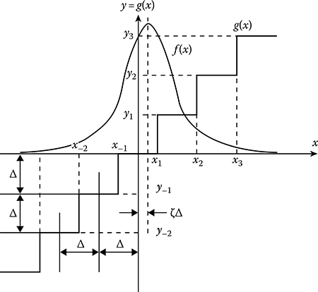
FIGURE 12.12 Staircase characteristic of quantization.

Images

FIGURE 12.13 Rectangular function.

where T_k = Σ_iτ_i is the total time when the observed realization is within the limits of the interval (k ± 0.5)Δ during its observation within the limits of the interval [0, T]. In doing so, $\lim_{T \to \infty} \frac{T_{k}}{T}$ is the probability that the stochastic process is within the limits of the interval (k ± 0.5)Δ.

The mathematical expectation of the realization y(t) forming at the output of inertialess element (transducer) with the transform characteristic given by (12.228) when the realization x(t) of the stochastic process ξ(t) excites the input of inertialess element is equal to the mathematical expectation of the mathematical expectation estimate given by (12.229) and is defined as

$〈 E 〉 = \int_{- \infty}^{\infty} g (x) p (x) d x = Δ \sum_{k = - \infty}^{\infty} k \int_{(k - 0.5) Δ}^{(k + 0.5) Δ} p (x) d x, (12.230)$

where p(x) is the one-dimensional pdf of the observed stochastic process. In general, the mathematical expectation of estimate 〈E〉 differs from the true value E₀; that is, as a result of quantization we obtain the bias of the mathematical expectation of the mathematical expectation estimate defined as

$b (E) = 〈 E 〉 - E_{0} . (12.231)$

To determine the variance of the mathematical expectation estimate according to (12.116), there is a need to define the correlation function of process forming at the transducer output, that is,

$R_{y} (τ) = \int_{- \infty}^{\infty} \int_{- \infty}^{\infty} g (x_{1}) g (x_{2}) p_{2} (x_{1}, x_{2}; τ) d x_{1} d x_{2} - {〈 E 〉}^{2}, (12.232)$

where p₂(x₁, x₂; τ) is the two-dimensional pdf of the observed stochastic process.

Since the mathematical expectation and the correlation function of process forming at the transducer output depend on the observed stochastic process pdf, the characteristics of the mathematical expectation estimate of stochastic process quantized by amplitude depend both on the correlation function and on the pdf of observed stochastic process.

Apply the obtained results to the Gaussian stochastic process with the one-dimensional pdf given by (12.153) and the two-dimensional pdf takes the following form:

$p_{2} (x_{1}, x_{2}; τ) = \frac{1}{2 π σ^{2} \sqrt{1 - R^{2} (τ)}} \exp {- \frac{{(x_{1} - E_{0})}^{2} + {(x_{2} - E_{0})}^{2} - 2 R (τ) (x_{1} - E_{0}) (x_{2} - E_{0})}{2 σ^{2} [1 - R^{2} (τ)]}} . (12.233)$

Define the mathematical expectation E₀ using the quantization step Δ:

$E_{0} = (c + d) Δ, (12.234)$

where c is the integer; −0.5 < d < 0.5. The value dΔ is equal to the deviation of the mathematical expectation from the middle of quantization interval (step). Further, we will take into consideration that for the considered staircase characteristic of transducer (transformer) the following relation is true:

$g (x + w Δ) = g (x) + w Δ, (12.235)$

where w = 0, ±1, ±2,… is the integer. Substituting (12.153) into (12.230) and taking into consideration (12.234) and (12.235), we can define the conditional mathematical expectation in the following form:

$\begin{matrix} 〈 E | d 〉 & = \frac{1}{\sqrt{2 π σ^{2}}} \int_{- \infty}^{\infty} g (x) \exp {- \frac{{[(x - c Δ) - d Δ]}^{2}}{2 σ^{2}}} d x \\ = \sum_{k = - \infty}^{\infty} k Δ {Q [(k - 0.5 - d) λ] - Q [(k + 0.5 - d) λ]} + c Δ, \end{matrix} (12.236)$

where

$λ = \frac{Δ}{σ} (12.237)$

is the ratio between the quantization step and root-mean-square deviation of stochastic process; Q(x) is the Gaussian Q function given by (12.68).

The conditional bias of the mathematical expectation estimate can be presented in the following form:

$b (E | d) = Δ \sum_{k = - \infty}^{\infty} k {Q [(k - 0.5 - d) λ] - Q [(k + 0.5 - d) λ]} - d Δ . (12.238)$

It is easy to see that the conditional bias is the odd function d, that is,

$b (E | d) = - b (E | - d), (12.239)$

and at that, if d = 0 and d = ±0.5, the mathematical expectation estimate is unbiased. If λ ≫ 1, in practice at λ ≥ 5, (12.238) is simplified and takes the following form:

$b (E | d) = {Q [0.5 λ (1 - 2 d)] - Q [0.5 λ (1 + 2 d)] - d} Δ . (12.240)$

At λ < 1, the conditional bias can be simplified. For this purpose, we can expand the function in braces in (12.238) into the Taylor series about the point (k − d)λ, but limit to the first three terms of expansion. As a result, we obtain

$b (E | d) = \frac{λ Δ}{\sqrt{2 π}} \sum_{k = - \infty}^{\infty} k \exp {- 0.5 {(k - d)}^{2} λ^{2}} - d Δ . (12.241)$

If λ ≪ 1, the sum in (12.241) can be changed by the integral. Denoting x = λk and dx = λ, we obtain

$\sum_{k = - \infty}^{\infty} k λ \exp {- 0.5 {(k - d)}^{2} λ^{2}} \approx \frac{1}{λ} \int_{- \infty}^{\infty} x \exp {- 0.5 {(x - d λ)}^{2}} d x = \sqrt{2 π} d . (12.242)$

As we can see from (12.241) and (12.242), at λ ≪ 1, that is, the quantization step is much lower than the root-mean-square deviation of stochastic process, the mathematical expectation estimate is unbiased for all practical training.

To obtain the unconditional bias we assume that d is the random variable uniformly distributed within the limits of the interval [−0.5; 0.5]. Let us take into consideration that

$\int Q (x) d x = x Q (x) - \int x Q' (x) d x . (12.243)$

Averaging (12.238) by all possible values of d we obtain

$b (E) = λ Δ \sum_{k = - \infty}^{\infty} k {2 k Q (k λ) - (k + 1) Q [(k + 1) λ] - (k - 1) Q [(k - 1) λ] + \frac{1}{\sqrt{2 π} λ} [- 2 \exp {- 0.5 λ^{2} k^{2}} + \exp {0.5 λ^{2} {(k + 1)}^{2}} + \exp {- 0.5 λ^{2} {(k - 1)}^{2}}]} . (12.244)$

The terms of expansion in series at k = p and k = −p are equal by module and are inverse by sign. Because of this, b(E) = 0; that is, the mathematical expectation estimate of stochastic process quantized by amplitude is unconditionally unbiased. Substituting (12.233) into (12.232), introducing new variables

${\begin{matrix} z_{1} & = x_{1} - c Δ, \\ z_{2} & = x_{2} - c Δ, \end{matrix} (12.245)$

and taking into consideration (12.235), we obtain

$R_{y} (τ) = \int_{- \infty}^{\infty} \int_{- \infty}^{\infty} g (z_{1}) g (z_{2}) p_{2} (z_{1}, z_{2}; τ) d z_{1} d z_{2}, (12.246)$

where p₂(z₁, z₂; τ) is the two-dimensional pdf of Gaussian stochastic process with zero mathematical expectation. To determine (12.246) we can present the two-dimensional pdf as expansion in series by derivatives of the Gaussian Q function (12.156) assuming that x = z and E₀ = 0 for the last formula. Substituting (12.156) and (12.228) into (12.246) and taking into consideration a parity of the function Q⁽¹⁾(z/σ) and oddness of the function g(z), we obtain

$R_{y} (τ) = \frac{1}{σ^{2}} \sum_{v = 1}^{\infty} \frac{R^{v} (τ)}{v!} {\int_{- \infty}^{\infty} g (z) Q^{(v + 1)} (\frac{z}{σ}) d z}^{2} . (12.247)$

Taking the integral in the braces by parts and taking into consideration that Q^(v)(±∞) = 0 at ν ≥ 1, we obtain

$\int_{- \infty}^{\infty} g (z) Q^{(v + 1)} (\frac{z}{σ}) d z = - σ \int_{- \infty}^{\infty} g' (z) Q^{(v)} (\frac{z}{σ}) d z . (12.248)$

According to (12.228),

$g' (z) = \frac{d g (z)}{d z} = \sum_{k = 1}^{\infty} Δ δ [z - (k - 0.5) Δ] + \sum_{k = - \infty}^{- 1} Δ δ [z - (k + 0.5) Δ], (12.249)$

where δ(z) is the Dirac delta function. Then the correlation function given by (12.247) takes the following form:

$R_{y} (τ) = Δ^{2} \sum_{v = 1}^{\infty} \frac{a_{v}^{2} R^{v} (τ)}{v!}, (12.250)$

where

$a_{v} = \sum_{k = 1}^{\infty} Q^{(v)} [(k - 0.5) λ] + \sum_{k = - \infty}^{- 1} Q^{(v)} [(k + 0.5) λ], (12.251)$

and at that the coefficients a_v are equal to zero at even v; that is, we can write

$a_{v} = {\begin{matrix} 2 \sum_{k = 1}^{\infty} Q^{(v)} [(k - 0.5) λ] & at & odd v, \\ 0 & at & even v . \end{matrix} (12.252)$

Substituting (12.250) into (12.116) and taking into consideration (12.252), we obtain the normalized variance of the mathematical expectation estimate of stochastic process:

$\frac{Var (E)}{σ^{2}} = 4 λ^{2} \sum_{v = 1}^{\infty} \frac{C_{2 v - 1}^{2}}{(2 v - 1)!} \times \frac{2}{T} \int_{0}^{T} (1 - \frac{τ}{T}) R^{2 v - 1} (τ) d τ, (12.253)$

where

$C_{2 v - 1} = \sum_{k = 1}^{\infty} Q^{(2 v - 1)} [(k - 0.65) λ] . (12.254)$

In the limiting case as Δ → 0, we have

$\begin{matrix} \lim_{Δ \to 0} \frac{Δ}{σ} C_{2 v - 1} & = \lim_{Δ \to 0} \frac{Δ}{σ} \sum_{k = 1}^{\infty} Q^{(2 v - 1)} [(k - 0.5) \frac{Δ}{σ}] \\ = \int_{0}^{\infty} Q^{(2 v - 1)} (z) d z = Q^{(2 v - 2)} (x) |_{0}^{\infty} = {\begin{matrix} 0.5 & if & v = 1, \\ 0 & if & v \geq 2. \end{matrix} \end{matrix} (12.255)$

As we can see from (12.253), based on (12.255) we obtain (12.116). Computations carried out, λC_2v−1, for the first five magnitudes v show that at λ ≤ 1.0 the formula (12.255) is approximately true with the relative error less than 0.02. Taking into consideration this statement, we observe a limitation caused by the first term in (12.253) for the indicated magnitudes A, especially for the reason that the contribution of terms with higher order in the total result in (12.253) decreases proportionally to the factors $λ^{2} C_{2 v - 1}^{2} / (2 v - 1)!$ Thus, if the quantization step is not more than the root-mean-square deviation of the observed Gaussian stochastic process, (12.116) is approximately true for the definition of the variance of mathematical expectation estimate.

12.7 Optimal Estimate of Varying Mathematical Expectation of Gaussian Stochastic Process

Consider the estimate of varying mathematical expectation E(t) of Gaussian stochastic process ξ(t) based on the observed realization x(t) within the limits of the interval [0, T]. At that time, we assume that the centralized stochastic process ξ₀(t) = ξ(t) − E(t) is the stationary stochastic process and the time-varying mathematical expectation of stochastic process can be approximated by a linear summation in the following form:

$E (t) \approx \sum_{i = 1}^{N} α_{i} φ_{i} (t), (12.256)$

where

α_i indicates unknown factors
φ_i(t) is the given function of time

If the number of terms in (12.256) is finite, that is, if N is finite, there will be a difference between E (t) and expansion in series. However, with increasing N, the error of approximation tends to approach zero:

$ε^{2} = \int_{0}^{T} {[E (t) - \sum_{i = 1}^{N} α_{i} φ_{i} (t)]}^{2} d t . (12.257)$

In this case, we say that the series given by (12.256) approaches the average.

Based on the condition of approximation error square minimum, we conclude that the factors α_i are defined from the system of linear equations:

$\sum_{i = 1}^{N} α_{i} \int_{0}^{T} φ_{i} (t) φ_{j} (t) d t = \int_{0}^{T} E (t) φ_{j} (t) d t, j = 1, 2, \dots, N . (12.258)$

In the case of representation E(t) in the series form (12.256), the functions φ_i(t) are selected in such a way to ensure fast series convergence. However, in some cases, the main factor in selection of the functions φ(t) is the simplicity of physical realization (generation) of these functions. Thus, the problem of definition of the mathematical expectation E(t) of stochastic process ξ(t) by a single realization x(t) within the limits of the interval [0, T] is reduced to estimation of the coefficients α_i in the series given by (12.256). In doing so, the bias and dispersion of the mathematical expectation estimate E(t) of the observed stochastic process caused by measurement errors of the coefficients α_i are given in the following form:

$b_{E} (t) = E (t) - E * (t) = \sum_{i = 1}^{N} φ_{i} (t) (α_{i} - 〈 α_{i}^{*} 〉); (12.259)$

$D_{E} (t) = \sum_{i = 1, j = 1}^{N} φ_{i} (t) φ_{j} (t) 〈 (α_{i} - α_{i}^{*}) (α_{j} - α_{j}^{*}) 〉, (12.260)$

where $α_{i}^{*}$ is the estimate of the coefficients α_i. Statistical characteristics (the bias and dispersion) of the mathematical expectation estimate of stochastic process averaged within the limits of the observation interval [0, T] take the following form:

$b_{E} (t) = \frac{1}{T} \int_{0}^{T} b_{E} (t) d t = \frac{1}{T} \sum_{i = 1}^{N} (α_{i} - 〈 α_{i}^{*} 〉) \int_{0}^{T} φ_{i} (t) d t; (12.261)$

$D_{E} (t) = \frac{1}{T} \int_{0}^{T} D_{E} (t) d t = \sum_{i = 1, j = 1}^{N} 〈 (α_{i} - α_{i}^{*}) (α_{j} - α_{j}^{*}) 〉 \frac{1}{T} \int_{0}^{T} φ_{i} (t) φ_{j} (t) d t . (12.262)$

The functional of the observed stochastic process pdf with accuracy, until the terms remain independent of the unknown mathematical expectation E(t), can be presented by analogy with (12.4) in the following form:

$F [x (t) | E (t)] = B_{1} \exp {\sum_{i = 1}^{N} α_{i} y_{i} - \frac{1}{2} \sum_{i = 1, j = 1}^{N} α_{i} α_{j} c_{i j}}, (12.263)$

where

$y_{i} = \int_{0}^{T} x (t) υ_{i} (t) d t = \int_{0}^{T} \int_{0}^{T} x (t_{1}) φ_{i} (t_{2}) ϑ (t_{1}, t_{2}) d t_{1} d t_{2}; (12.264)$

$c_{i j} = c_{j i} = \int_{0}^{T} φ_{i} (t) υ_{i} (t) d t = \int_{0}^{T} \int_{0}^{T} φ_{i} (t_{1}) φ_{j} (t_{2}) ϑ (t_{1}, t_{2}) d t_{1} d t_{2}, (12.265)$

and the function υ_i(t) is defined by the following integral equation:

$\int_{0}^{T} R (t, τ) υ_{i} (τ) d τ = φ_{i} (t) . (12.266)$

Solving the likelihood equation with respect to unknown coefficients α_i

$\frac{\partial F [x (t) | E (t; α_{1}, \dots, α_{N})]}{\partial α_{j}} = 0, (12.267)$

we can find the system of N linear equations

$\sum_{i = 1}^{N} α_{i}^{*} c_{i j} = y_{j}, j = 1, 2, \dots, N (12.268)$

with respect to the estimates $α_{i}^{*}$ . Based on (12.268), we can obtain the estimates of coefficients

$α_{m}^{*} = \frac{A_{m}}{A} = \frac{1}{A} \sum_{i = 1}^{N} A_{m_{i}} y_{i}, m = 1, 2, \dots, N, (12.269)$

where

$A = ‖ c_{i j} ‖ = | \begin{matrix} c_{11} & c_{12} & \dots & c_{1 m} & \dots & c_{1 N} \\ c_{21} & c_{22} & \dots & c_{2 m} & \dots & c_{2 N} \\ ⋮ & ⋮ & ⋮ & ⋮ \\ c_{N 1} & c_{N 2} & \dots & c_{N m} & \dots & c_{N N} \end{matrix} | (12.270)$

is the determinant of the system of linear equations given by (12.268),

$A_{m} = | \begin{matrix} c_{11} & c_{12} & \dots & y_{1} & \dots & c_{1 N} \\ c_{21} & c_{22} & \dots & y_{2} & \dots & c_{2 N} \\ ⋮ & ⋮ & ⋮ & ⋮ \\ c_{N 1} & c_{N 2} & \dots & y_{N} & \dots & y_{N N} \end{matrix} | (12.271)$

is the determinant obtained from the determinant A given by (12.270) by changing the column c_im by the column y_i; A_im is the algebraic supplement of the mth column elements (the column y_i). In doing so, the following relationship

$\sum_{j = 1}^{N} c_{i j} A_{k j} = \sum_{j = 1}^{N} c_{i j} A_{j k} = A δ_{i k} (12.272)$

is true for the quadratic matrix ||c_ij||.

A flowchart of the optimal measurer of varying mathematical expectation of Gaussian stochastic process is shown in Figure 12.14. The measurer operates in the following way. Based on the previously mentioned system of functions φ_i(t) generated by the “Gen_φ” and a priori information about the correlation function R(τ) of observed stochastic process, the generator “Gen_v” forms the system of linear functions v_i(t) in accordance with the integral equation (12.266). According to (12.265), the generator “Gen_C” generates the system of coefficients c_ij sent to “Microprocessor”. The magnitudes y_i come in at the input of “Microprocessor” and also from the outputs of the “Integrator”. Based on a solution of N linear equations given by (12.268) with respect to unknown coefficients α_i, the “Microprocessor” generates their estimates. Using the estimates $α_{i}^{*}$ and system of functions φ_i(t), the estimate E*(t) of time-varying mathematical expectation E(t) is formed according to (12.256). The generated estimate E(t) will have a delay with respect to the true value on T + ΔT that is required to compute the random variables y_i and to solve the m linear equations by “Microprocessor”. The delay blocks T and ΔT are used by the flowchart with this purpose.

Substituting x(t) given by (12.2) into (12.264), we can write

$y_{i} = \int_{0}^{T} x_{0} (t) υ_{i} (t) d t + \int_{0}^{T} E (t) υ_{i} (t) d t = n_{i} + α_{m} c_{i m} + \sum_{q = 1, q \neq m}^{N} α_{q} c_{i q}, (12.273)$

where

$n_{i} = \int_{0}^{T} x_{0} (t) υ_{i} (t) d t . (12.274)$

Images

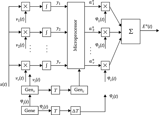
FIGURE 12.14 Optimal measurer of time-varying mathematical expectation estimate.

Taking into consideration (12.272) and (12.273), the determinant given by (12.271) can be presented in the form of sum of two determinants

$A_{m} = B_{m} + C_{m}, (12.275)$

where

$B_{m} = | \begin{matrix} c_{11} & c_{12} & \dots & (n_{1} + α_{m} c_{1 m}) & \dots & c_{1 N} \\ c_{21} & c_{22} & \dots & (n_{2} + α_{m} c_{2 m}) & \dots & c_{2 N} \\ ⋮ & ⋮ & ⋮ & ⋮ \\ c_{N 1} & c_{N 2} & \dots & (n_{N} + α_{m} c_{N m}) & \dots & c_{N N} \end{matrix} |, (12.276)$

The determinant C_m is obtained from the determinant B_m by changing the mth column on the column consisting of the terms $\sum_{q = 1, q \neq m}^{N} α_{q} c_{i q}$ at q ≠ m. Since the mth column of the determinant C_m consists of two elements that are the linear combination of elements of other columns, then C_m = 0.

Let us present the determinant A_m = B_m in the form of sum of products of all elements of the mth column on their algebraic supplement A_m, that is,

$A_{m} = \sum_{i = 1}^{N} (n_{i} + α_{m} c_{i m}) A_{i m} . (12.277)$

Taking into consideration that

$\sum_{i = 1}^{N} A_{i m} c_{i m} = A, (12.278)$

the estimate of the coefficients α_m takes the following form:

$α_{m}^{*} = \frac{1}{A} \sum_{i = 1}^{N} A_{i m} n_{i} + α_{m}, m = 1, 2, \dots, N . (12.279)$

Since

$〈 n_{i} 〉 = \int_{0}^{T} 〈 x_{0} (t) 〉 υ_{i} (t) d t = 0, (12.280)$

the estimates of the coefficients α_i of series given by (12.256) are unbiased. The correlation function of estimates of the coefficients α_m and α_q is defined by the following form:

$R (α_{m}, α_{q}) = \frac{1}{A^{2}} \sum_{i = 1, j = 1}^{N} 〈 n_{i} n_{j} 〉 A_{i m} A_{j q} = \frac{A_{m q}}{A} . (12.281)$

While delivering (12.281), we have taken into consideration the integral equation (12.266) and the formula given by (12.272). Now, we are able to define the variance of estimate of the coefficients. α_m, namely,

$Var (α_{m}) = \frac{A_{m m}}{A} . (12.282)$

In practice, we can assume that the frequency band Δf_E of the varying mathematical expectation is much less the effective frequency band Δf_ef of the spectrum G(f) of the observed centralized stochastic process ξ₀(t), and the spectrum G(f) is not changed for all practical training within the limits of the frequency band Δf_E. In this case, the centralized stochastic process ξ₀(t) can be considered as the “white” noise with the effective spectral density

$N_{ef} = \int_{0}^{Δ f_{E}} \frac{G (f)}{Δ f_{E}} d f (12.283)$

for further analysis. In doing so, the effective spectrum bandwidth can be defined as

$Δ f_{ef} = \int_{0}^{\infty} \frac{G (f)}{G_{max} (f)} d f . (12.284)$

In the case of accepted approximation, the correlation function of the centralized stochastic process. ξ₀(t) is approximated by

$R (τ) = \frac{N_{ef}}{2} δ (τ) . (12.285)$

Substituting (12.285) into the integral equation (12.266), we obtain

$υ_{i} (t) = \frac{2}{N_{ef}} φ_{i} (t) . (12.286)$

In doing so, the matrix of the coefficients

$c_{i j} = \frac{2}{N_{ef}} δ_{i j} (12.287)$

is the diagonal matrix and the determinant and algebraic supplement of this matrix are defined, correspondingly

$A = {\frac{2}{N_{ef}}}^{N}; (12.288)$

$A_{i m} = {\begin{array}{l} A_{m m} = {\frac{2}{N_{ef}}}^{N - 1}, & at & i = m, \\ 0, & at & i \neq m . \end{array} (12.289)$

As we can see from (12.281), the correlation function of the estimates $α_{m}^{*}$ and $α_{q}^{*}$ takes the following form:

$R (α_{m}^{*}, α_{q}^{*}) = \frac{N_{ef}}{2} δ_{m q} . (12.290)$

Based on (12.260), (12.262), and (12.290), we can note that the current and averaged variances of the varying mathematical expectation estimate E*(t) can be presented in the following form:

${Var}_{E*} (t) = \frac{N_{ef}}{2} \sum_{i = 1}^{N} φ_{i}^{2} (t), (12.291)$

$Var (E *) = \frac{1}{T} \sum_{i = 1}^{N} Var (α_{i}) = \frac{N_{ef}^{N}}{2 T} . (12.292)$

As we can see from (12.292), the higher the number of terms under expansion in series in (12.256) used for approximation of the mathematical expectation, the higher the variance of time-varying mathematical expectation estimate at the same conditions averaged within the limits of the observation interval. In doing so, there is a need to note that in general, the number N of series expansion terms essentially increases corresponding to the increase in the observation interval [0, T], within the limits of which the approximation is carried out.

As applied to the correlation function given by (12.13), the effective spectral density of the centralized stochastic process ξ(t) takes the following form:

$N_{ef} = \frac{2 σ^{2}}{π Δ f_{E}} arctg (\frac{2 π Δ f_{E}}{α}) . (12.293)$

If the observed stochastic process is stationary, then

$N_{ef} = \frac{4 σ^{2}}{α} and v = 1, (12.294)$

and the variance of the mathematical expectation estimate takes a form given by (12.50). The formulae for the variance of estimates of the coefficients α_m given by (12.282) and the variance of the time-varying mathematical expectation E(t) given by (12.260) and (12.262) are simplified essentially if the functions φ(t) satisfy the integral Fredholm equation of the second kind:

$φ_{i} (t) = λ_{i} \int_{0}^{T} R (t, τ) φ_{i} (τ) d τ . (12.295)$

In the considered case, the coefficients λ_i and the functions φ_i(t) are called the eigenvalues and eigenfunctions of the integral equation, respectively. Comparing (12.295) and (12.266), we can see

$υ_{i} (t) = λ_{i} φ_{i} (t) . (12.296)$

In theory of stochastic processes [15–17], it is proved that if the functions ϕ_i(t) were to satisfy the Equation 12.295, then these functions are the orthogonal normalized (orthonormalized) functions and the eigenvalues λ_i > 0. In this case, the following equation

$\int_{0}^{T} φ_{i} (t) φ_{j} (t) d t = δ_{i j} = {\begin{array}{l} 1 & if & i = j, \\ 0 & if & i \neq j \end{array} (12.297)$

is true for the eigenfunctions φ_i(t), and the correlation function R (t₁, t₂) can be presented by the following expansion in series

$R (t_{1}, t_{2}) = \sum_{i = 1}^{\infty} \frac{φ_{i} (t_{1}) φ_{i} (t_{2})}{λ_{i}}, (12.298)$

and the following equality is satisfied:

$\sum_{i = 1}^{\infty} \frac{1}{λ_{i}} = σ^{2} T . (12.299)$

Substituting (12.295) into (12.265) and taking into consideration (12.297), we obtain

$c_{i j} = {\begin{array}{l} λ_{i} & if & i = j, \\ 0 & if & i \neq j . \end{array} (12.300)$

At that, the matrix of coefficients c_ij = λ_i is the diagonal matrix. The determinant A and the algebraic supplements A_m of this matrix can be presented in the following form, respectively,

$A = \prod_{i = 1}^{N} λ_{i}, (12.301)$

$A_{i m} = {\begin{array}{l} \frac{A}{λ_{m}} & if & i = m, \\ 0 & if & i \neq m . \end{array} (12.302)$

As we can see from (12.301), (12.302), (12.269), and (12.256), the estimates of the coefficients $α_{i}^{*}$ and the time-varying mathematical expectation estimate E*(t) can be presented in the following form:

$α_{i}^{*} = \int_{0}^{T} x (τ) φ_{i} (τ) d τ; (12.303)$

$E * (t) = \sum_{i = 1}^{N} α_{i}^{*} φ_{i} (t) . (12.304)$

Images

FIGURE 12.15 Optimal measurer of time-varying mathematical expectation estimate in accordance with (12.304); particular case of the flowchart in Figure 12.14.

The optimal measurer of the time-varying mathematical expectation of Gaussian stochastic process operating in accordance with (12.304) is shown in Figure 12.15. The flowchart presented in Figure 12.15 is a particular case of the measurer depicted in Figure 12.14. Based on the well-known correlation function of the observed stochastic process, in accordance with (12.295), the generator “Gene” forms the functions φ_i(t) that are employed to form the coefficients $α_{i}^{*}$ . The estimates of coefficients are multiplied by the functions φ_i(t) again and obtained products come in at the summator input. The expected estimate E*(t) of the time-varying mathematical expectation is formed at the summator output. Delay is required to compute the coefficients $α_{i}^{*}$ .

The variance of estimate of the coefficients $α_{i}^{*}$ and the current and averaged variances of estimates E*(t) of the time-varying mathematical expectation are transformed in accordance with (12.282), (12.260), and (12.262) in the following form:

$Var (α_{m}^{*}) = \frac{1}{λ_{m}}; (12.305)$

$Var {E * (t)} = \sum_{i = 1}^{N} \frac{φ_{i}^{2} (t)}{λ_{i}}; (12.306)$

$Var (E *) = \sum_{i = 1}^{N} \frac{1}{λ_{i} T} . (12.307)$

As we can see from (12.307), with increase in the number of terms under approximation E(t) by the series given by (12.256), the averaged variance of the time-varying mathematical expectation estimate E* also increases. As N → ∞, taking into consideration (12.299), we obtain

$Var (E *) = σ^{2} . (12.308)$

Thus, at a sufficiently large number of the eigenfunctions in the sum given by (12.256), the averaged variance of the time-varying mathematical expectation estimate E (t) is equal to the variance of the initial stochastic process. In doing so, the estimate bias caused by the finite number of terms in series given by (12.256) tends to approach zero. However, in practice, there is a need to choose the number of terms in series given by (12.256) in such a way that a dispersion of the time-varying mathematical expectation estimate caused both by the bias and by the estimate variance would be minimal.

12.8 Varying Mathematical Expectation Estimate Under Stochastic Process Averaging in Time

The problems with using optimal procedure realizations to estimate the time-varying mathematical expectations of stochastic processes are common in sufficiently complex mathematical computations. For this reason, to measure the time-varying mathematical expectations of stochastic processes in the course of practical applications, the averaging in time of the observed stochastic process is widely used. In principle, to define the current value of the mathematical expectation of nonstationary stochastic process there is a need to have a set of realizations x_i(t) of the investigated stochastic process ξ(t). Then, the estimate of searched parameter of the stochastic process at the instant t₀ is determined in the following form:

$E * (t_{0}) = \frac{1}{N} \sum_{i = 1}^{N} x_{i} (t_{0}), (12.309)$

where N is the number of investigated stochastic process realizations. As we can see from (12.309), the mathematical expectation estimate is unbiased and the variance of the mathematical expectation estimate can be presented in the following form:

$Var [E * (t)] = \frac{σ^{2} (t_{0})}{N}, (12.310)$

in the case of independent realizations x_i(t), where σ²(t₀) is the variance of investigated stochastic process at the instant t = t₀. Thus, the estimate given by (12.309) is the consistent since N → ∞ the variance of estimate tends to approach zero. However, as a rule, a researcher does not use a sufficient number of realizations of stochastic process; thus, there is a need to carry out an estimation of the mathematical expectation based on an analysis of the limited number of realizations and, sometimes, based on a single realization.

Under definition of estimation of the time-varying mathematical expectation of stochastic process by a single realization, we meet with difficulties caused by the definition of optimal time of averaging (integration) or the time constant of smoothing filter at the earlier-given filter impulse response. In doing so, two conflicting requirements arise. On one hand, there is a need to decrease the variance of estimate caused by finite time interval of measuring; this time interval must be large. On the other hand, for better distinguishing the mathematical expectation variations in time, there is a need to choose the integration time as short as possible. Evidently, there is an optimal averaging time or the bandwidth of the smoothing filter under the given impulse response, which corresponds to minimal dispersion of the mathematical expectation estimate of stochastic process caused by the aforementioned factors.

The simplest way to define the mathematical expectation of stochastic process at the instant t = t₀ is an averaging of ordinates of stochastic process realization within the limits of time interval about the given magnitude of argument t = t₀. In doing so, the mathematical expectation estimate is defined as

$E * (t_{0}, T) = \frac{1}{T} \int_{t_{0} - 0.5 T}^{t_{0} + 0.5 T} x (t) d t = \frac{1}{T} \int_{- 0.5 T}^{0.5 T} x (t_{0} + t) d t . (12.311)$

Averaging (12.311) by realizations, we obtain the mathematical expectation of estimate at the instant t = t₀:

$〈 E * (t_{0}, T) 〉 = \frac{1}{T} \int_{- 0.5 T}^{0.5 T} E (t_{0} + t) d t, (12.312)$

where E(t₀ + t) is the true mathematical expectation value of the investigated stochastic process at the instant t = t₀. Thus, the mathematical expectation of estimate of the time-varying mathematical expectation of stochastic process in contrast to the stationary case is obtained by smoothing the estimate within the limits of time interval [t₀ − 0.5T; t₀ + 0.5T].

In general, as a result of considered averaging, there is the mathematical expectation bias that can be presented in the following form:

$b [E * (t_{0}, T)] = \frac{1}{T} \int_{- 0.5 T}^{0.5 T} [E (t_{0} + t) - E (t_{0})] d t . (12.313)$

If the magnitude E(t) is described about the point t = t₀ within the limits of time interval [t₀ − 0.5T; t₀ + 0.5T] by the series with odd powers in the following form

$E (t + t_{0}) \approx E (t_{0}) + \sum_{k = 1}^{N} \frac{t^{2 k - 1}}{(2 k - 1)!} {[\frac{d^{(2 k - 1)} E (t)}{d t^{(2 k - 1)}}]}_{t_{0}}, (12.314)$

the mathematical expectation estimate bias would be minimal. Then

$b [E * (t_{0}, T)] \approx 0. (12.315)$

The variance of the mathematical expectation estimate of the investigated stochastic process is defined in the following form:

$Var [E * (t_{0}, T)] = \frac{1}{T^{2}} \int_{- 0.5 T}^{0.5 T} \int_{- 0.5 T}^{0.5 T} R (t_{0} + t_{1}, t_{0} + t_{2}) d t_{1} d t_{2}, (12.316)$

where R(t₁, t₂) is the correlation function of the investigated stochastic process ξ(t).

In practice, the nonstationary stochastic processes with time-varying mathematical expectation or variance or both of them simultaneously are widely used. In doing so, the mathematical expectation and variance vary slowly in comparison with variations of the investigated stochastic process. In other words, the mathematical expectation and variance of stochastic process are constant within the limits of the correlation interval. In this case, to define the variance of the time-varying mathematical expectation estimate we can assume that the centralized stochastic process ξ₀(t) = ξ(t) −E(t) is the stationary stochastic process within the limits of the interval t₀ ± 0.5T with the correlation function that can be presented in the following form:

$R (τ) = 〈 ξ_{0} (t) ξ_{0} (t + τ) 〉 \approx σ^{2} (t_{0}) ℛ (τ) . (12.317)$

Taking into consideration the given approximation, the variance of the mathematical expectation estimate given by (12.316) after transformation of the double integral by introducing new variables τ = t₂ − t₁, t₂ = t and changing the order of integration takes the following form:

$Var [E * (t_{0}, T)] \approx σ^{2} (t_{0}) \times \frac{2}{T} \int_{0}^{T} (1 - \frac{τ}{T}) ℛ (τ) d τ . (12.318)$

As we can see from (12.313) and (12.318), the dispersion of the mathematical expectation estimate is defined in the following form:

$D [E * (t_{0}, T)] = b^{2} [E * (t_{0}, T)] + Var [E * (t_{0}, T)] . (12.319)$

In principle, we can define the optimal integration time T, under which the dispersion will be minimum at the instant t₀ minimizing the dispersion of estimate by the parameter T. However, we can present a solution to this problem in an acceptable analytical form by giving a specific function of E(t). Evaluate how the mathematical expectation estimate varies when the mathematical expectation E(t) deviates from the linear function. At the same time, we assume that the estimated mathematical expectation E(t) possesses the first and second continuous derivatives with respect to the time t. Then, according to the Taylor formula, we can write

$E (t) = E (t_{0}) + (t - t_{0}) E' (t_{0}) + 0.5 {(t - t_{0})}^{2} E ″ [t_{0} + ϑ (t - t_{0})], (12.320)$

where 0 < ϑ < 1. Substituting (12.320) into (12.313), we obtain

$b [E * (t_{0}, T)] = \frac{1}{2 T} \int_{- 0.5 T}^{0.5 T} t^{2} E ″ [t_{0} + t ϑ] d t . (12.321)$

Denoting M as the maximum value of the second derivative of the mathematical expectation E (t) with respect to the time t, we obtain the top bound of the mathematical expectation estimate bias by module

$| b [E * (t_{0}, T)] | \leq \frac{T^{2} M}{24} . (12.322)$

As a rule, the maximum magnitude of the second derivative of the mathematical expectation E(t) with respect to the time t can be evaluated based on an analysis of specific physical problems.

To estimate the optimal time of integration T minimizing the dispersion of estimate given by (12.319), we assume that the correlation interval of the investigated stochastic process is much less than the integration time, that is, τ_cor ≪ T. Then, the following written form is true:

$\int_{0}^{T} (1 - \frac{τ}{T}) ℛ (τ) d τ \approx \int_{0}^{\infty} ℛ (τ) d τ \leq \int_{0}^{\infty} | ℛ (τ) | d τ = τ_{cor} . (12.323)$

Taking into consideration (12.322) and (12.323) and based on the condition of minimization of the estimate dispersion given by (12.319), we obtain the optimal estimation of the integration time:

$T \approx 2 {[\frac{9 σ^{2} (t_{0}) τ_{cor}}{M^{2}}]}^{\frac{1}{5}} . (12.324)$

As we can see from (12.324), the larger the integration time, the larger the correlation interval and the variance of the investigated stochastic process. The lesser the integration time, the larger the maximum absolute value of the second derivative of the mathematical expectation measured. This statement agrees well with the physical interpretation of measuring the time-varying mathematical expectation.

In some applications, the time-varying mathematical expectation can be approximated by the series given by (12.256). The values minimizing the function

$ε^{2} (α_{1}, α_{2}, \dots, α_{N}) = \frac{1}{T} \int_{0}^{T} {[x (t) - \sum_{i = 1}^{N} α_{i} φ_{i} (t)]}^{2} d t (12.325)$

can be considered as the estimates of the coefficients $α_{i}^{*}$ . This representation of the coefficients $α_{i}^{*}$ is possible only if the mathematical expectation E(t) and the functions φ_i(t) vary in time slowly in comparison with the variation of the first derivative of the function x₀(t) with respect to the time; that is, the following condition must be satisfied:

$\begin{matrix} {| \frac{E' (t)}{E (t)} |}_{\max} \\ {| \frac{φ_{i}^{'} (t)}{φ_{i} (t)} |}_{max} \end{matrix}} ≪ \sqrt{\frac{〈 {[x_{0}^{'} (t)]}^{2} 〉}{σ^{2} (t)}} . (12.326)$

In other words, the condition (12.325) to define the coefficients $α_{i}^{*}$ is true if the frequency band Δf_E of the mathematical expectation E (t) is much less than the effective bandwidth of energy spectrum of the stochastic component x₀(t). Based on the condition of minimization the function ε², that is,

$\frac{d ε^{2}}{\partial α_{m}} = 0, (12.327)$

we obtain the system of equations to estimate the coefficients $α_{m}^{*}$

$\sum_{i = 1}^{N} α_{i}^{*} \int_{0}^{T} φ_{i} (t) φ_{m} (t) d t = \int_{0}^{T} x (t) φ_{m} (t) d t, m = 1, 2, \dots, N . (12.328)$

Denote

$\int_{0}^{T} φ_{i} (t) φ_{m} (t) d t = c_{i m}; (12.329)$

$\int_{0}^{T} x (t) φ_{m} (t) d t = y_{m} . (12.330)$

Then the estimations of the coefficients $α_{m}^{*}$ can be presented in the following form:

$α_{m}^{*} = \frac{A_{m}}{A}, m = 1, 2, \dots, N, (12.331)$

where the determinant A of the system of linear equations given by (12.328) and the determinant A_m obtained by changing the mth column c_im of the determinant A by the column y_i are determined based on (12.270) and (12.271).

The flowchart of measurer of the time-varying mathematical expectation estimate is similar to the block diagram shown in Figure 12.14, but the difference is that a set of functions φ(t) are assigned for the sake of convenience in generating them and the coefficients c_ij and values y_i are formed according to (12.329) and (12.330), correspondingly. Definition of the coefficients $α_{m}^{*}$ is simplified essentially if the functions φ(t) are orthonormal functions; that is, the formula (12.297) is true. In this case,

$α_{m}^{*} = \int_{0}^{T} x (t) φ_{m} (t) d t . (12.332)$

The flowchart of measurer of the time-varying mathematical expectation estimate differs from the block diagram shown in Figure 12.15, and the difference is that a set of functions φ_i(t) are assigned for the sake of convenience in generating them; thus, there is no need to solve the integral equation (12.295).

Compute the estimate bias and mutual correlation functions between the estimates of the coefficients $α_{m}^{*}$ and $α_{q}^{*}$ . Based on investigation carried out in Section 12.7, we can conclude that the estimations of the coefficients $α_{m}^{*}$ of expansion in series given by (12.256) are unbiased estimates and the correlation functions and variances of estimates of the coefficients $α_{m}^{*}$ are defined in the following form:

$R (α_{m}^{*}, α_{q}^{*}) = \frac{1}{A^{2}} \sum_{i = 1, j = 1}^{N} A_{i m} A_{j q} C_{i j}, (12.333)$

$Var (α_{m}^{*}) = \frac{1}{A^{2}} \sum_{i = 1, j = 1}^{N} A_{i m} A_{j m} C_{i j}, (12.334)$

where A_im is the algebraic supplement of the determinant given by (12.270),

$C_{i j} = \int_{0}^{T} \int_{0}^{T} R (t_{1}, t_{2}) φ_{i} (t_{1}) φ_{j} (t_{2}) d t_{1} d t_{2}, (12.335)$

and R(t₁, t₂) is the correlation function of the investigated stochastic process.

With φ_i(t) used as the orthonormal function, the coefficients c_im given by (12.329) take the following form:

$c_{i m} = δ_{i m} . (12.336)$

In doing so, the matrix ‖c_ij‖ is transformed to the diagonal matrix and the determinant A of this matrix and algebraic supplements A_ij are defined as follows:

$\begin{matrix} A = 1, & A_{i j} = δ_{i j} . \end{matrix} (12.337)$

Based on (12.336) and (12.333), the correlation function of estimation of the coefficients $α_{m}^{*}$ and $α_{q}^{*}$ can be presented in the following form:

$R (α_{m}^{*}, α_{q}^{*}) = C_{m q}, (12.338)$

where $C_{i j}$ is given by (12.335) at i = m, j = q. In doing so, the current variance of estimate given by (12.260) and the averaged variance of estimate (12.262) of the time-varying mathematical expectation take the following form:

$Var {E * (t)} = \sum_{i = 1, j = 1}^{N} C_{i j} φ_{i} (t) φ_{j} (t); (12.339)$

$Var {E *} = \frac{1}{T} \sum_{i = 1}^{N} C_{i i} . (12.340)$

correspondingly.

If it is possible to approximate the centralized stochastic process ξ₀(t) by the “white” noise with the effective spectral density given by (12.283) in addition to the orthonormal functions φ_i(t), then we can write

$C_{i j} = \frac{N_{ef}}{2} δ_{i j} . (12.341)$

Based on (12.341), we are able to define the current and averaged variances of the time-varying mathematical expectation estimates coinciding with the optimal estimations given by (12.336) and (12.338), which are applied to the observation of the Gaussian stochastic process with the time-varying mathematical expectation.

12.9 Estimate of Mathematical Expectation by Iterative Methods

Currently, the iterative methods or procedures of step-by-step approximation are widely used to estimate the parameters of stochastic processes. These procedures and methods are also called the recurrent procedures or methods of stochastic approximation. Essence of the iterative method applied to estimation of scalar parameter l by discrete sample with the size N is to form the recurrent relationship in the following form [18]:

$l * [N] = l * [N - 1] + γ [N] {f (x [N]) - l * [N - 1]}, (12.342)$

where

l*[N − 1] and l*[N] are the estimates of stochastic process parameter based on the observation of N − 1 and N samples, respectively
f(x[N]) is the function of received sample related with the transformation required to obtain the searched stochastic process parameter
γ[N] is the factor defining a value of next step to make accurate the estimate of parameter l, depending on the number of step N and satisfying the following conditions:

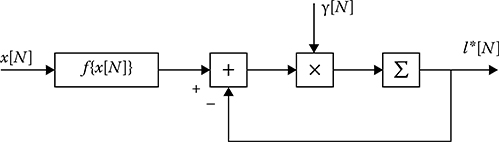
${\begin{array}{l} γ [N] > 0, \\ \sum_{N = 1}^{\infty} γ [N] \to \infty, \\ \sum_{N = 1}^{\infty} γ^{2} [N] < \infty . \end{array} (12.343)$

Images

FIGURE 12.16 Iterative measurer of mathematical expectation.

The relationship (12.342) allows us to image the flowchart of the iterative measurer of stochastic process parameter.

The discrete algorithm given by (12.342) can be transformed to the continuous algorithm using the limiting process for the difference equation

$l [N] - l [N - 1] = Δ l [N] = γ [N] {f (x [N]) - l [N - 1]} (12.344)$

to differential equation

$\frac{d l (t)}{d t} = γ (t) {f [x (t)] - l (t)} . (12.345)$

The flowchart of measurer corresponding to (12.345) is similar to the block diagram shown in Figure 12.16 where there is a need to change γ[N] on γ(t) and the summator on the integrator.

As applied to the mathematical expectation estimate of stationary stochastic process, the recur-rent algorithm of measurement takes the following form:

$E * [N] = E * [N - 1] + γ [N] {x [N] - E * [N - 1]} . (12.346)$

The optimal magnitude of the factor γ[N] to estimate the mathematical expectation of stochastic process by uncorrelated samples can be obtained from (12.182). This optimal value must ensure the minimal variance of the mathematical expectation estimate over the class of linear estimations given by (12.183). Actually, (12.182) can be presented in the following form:

$E * [N] = \frac{1}{N} \sum_{i = 1}^{N} x_{i} = E * [N - 1] + \frac{1}{N} {x [N] - E * [N - 1]} . (12.347)$

Comparing (12.346) and (12.347), we obtain the optimal magnitude of the factor γ[N]:

$γ_{opt} [N] = \frac{1}{N} . (12.348)$

The flowchart of iterative measurer of the mathematical expectation is similar to the block diagram shown in Figure 12.16, in which there is a need to exclude block f (x[N]) responsible for transformation of stochastic process.

Since the iterative algorithm (12.347) is equivalent to the algorithm (12.182), we can state that, in the considered case, the mathematical expectation estimate is unbiased and the variance of the mathematical expectation estimate is given by (12.183). In practice, we sometimes use the constant values of the factor, γ[N] that is,

$γ [N] = γ = const, 0 < γ < 1. (12.349)$

In this case, the estimation given by (12.346) can be presented in the following form [19, 20]:

$E * [N] = {(1 - γ)}^{N} x [1] + γ \sum_{i = 2}^{N} {(1 - γ)}^{N - i} x_{i} = {(1 - γ)}^{N} {x [1] + γ \sum_{i = 2}^{N} \frac{x_{i}}{{(1 - γ)}^{i}}} . (12.350)$

As we can see from (12.350), the mathematical expectation estimate is unbiased. To define the variance of estimate, we assume that the samples x_i are uncorrelated. Then, the variance of mathematical expectation estimate takes the following form:

$Var {E *} = \frac{2 {(1 - γ)}^{2 N - 1} + γ}{2 - γ} σ^{2} . (12.351)$

As 1 − γ < 1 and N → ∞ or N ≫ 1, (12.351) can be simplified and takes the limiting form:

$Var {E *} \approx \frac{γ}{2 - γ} σ^{2}, (12.352)$

that is, the considered estimate is not consistent.

The ratio between the variance of the mathematical expectation estimate defined by (12.351) and the variance of the optimal mathematical expectation estimate given by (12.183) as a function of the number of uncorrelated samples N and various magnitudes of the factor γ is shown in Figure 12.17. As we can see from Figure 12.17, for each value N there is a definite magnitude γ, at which the ratio of variances reaches the maximum.

Images

FIGURE 12.17 Ratio between the variance of mathematical expectation estimate given by (12.351) and the variance of optimal mathematical expectation estimate given by (12.183) as a function of the number of uncorrelated samples N and various values of the factor γv.

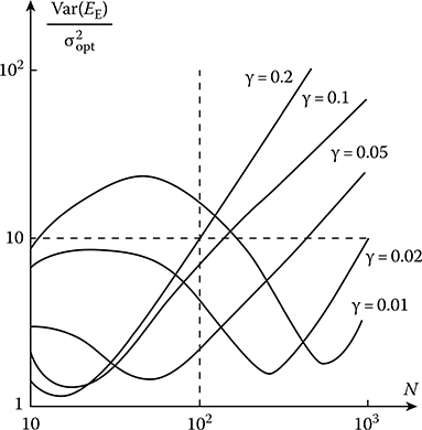
12.10 Estimate of Mathematical Expectation with Unknown Period

In some applications, we can suppose that the time-varying mathematical expectation E(t) of the stochastic process ξ(t) is the periodic function

$\begin{matrix} E (t) = E (t + k T_{0}), & k = 0, 1, \dots, \end{matrix} (12.353)$

and the value of the period T₀ is unknown. At the same time, the practical case, when the period T₀ is much more than the correlation interval τ_cor of the observed stochastic process, is of interest for us. We employ the adaptive filtering methods widely used in practice under interference cancellation to measure the time-varying mathematical expectation estimate [21]. We consider the discrete sample x(t_i) = x_i = x(iT_s) where the sampling period is T_s. The sample can be presented in the form discussed in (12.168).

The observed samples x_i come in at the inputs of the main and reference (the adaptive filter) channels (see Figure 12.18). The delay τ = kT_s, where k is integer, is chosen in such a way that the samples at the main and reference channels would be uncorrelated. There is a filter with varying parameters in the reference channel. The incoming samples x_i and the process y_i forming at the adaptive filter output are sent at the subtractor input. At the subtractor output, the following process

$ε_{i} = x_{i} - y_{i} = x_{0_{i}} + (E_{i} - y_{i}) (12.354)$

takes place. Taking into consideration that the samples are uncorrelated, the mathematical expectation of quadratic signal in the main and reference channels is defined as

$〈 ε^{2} 〉 = σ_{0}^{2} + 〈 {(E_{i} - y_{i})}^{2} 〉 . (12.355)$

The minimum of 〈ε²〉 corresponds to the minimum of the second term in the right side (12.355). Thus, if the parameters of adaptive filter are changed before definition of the minimum 〈ε²〉, there is a need to use the signal y_i at the adaptive filter output as the estimate $E_{i}^{*}$ of time-varying mathematical expectation. As was shown in Ref. [21], under the given structure of interference and noise canceller, the value y_i is the best estimate in the case of the quadratic loss function given by (11.25).

Images

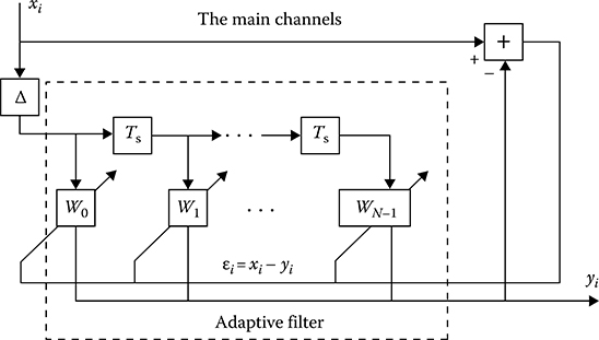
FIGURE 12.18 Adaptive filter flowcharts.

The adaptive filter with required impulse response is realized in the form of linear vector summing of signals with the weight coefficients W_j, where j = 0, 1,…, P − 1 are the numbers of parallel channels, at that, the delay between neighboring channels is equal to the sampling period T_s. Tuning of the weight coefficients $W_{j}^{*}$ is carried out in accordance with the recurrent Widrow-Hopf algorithm [22]

$W_{j}^{*} [N + 1] = W_{j}^{*} [N] + 2 μ {x [N] x [N - d - j] - x [N - d - j] \sum_{l = 0}^{P - 1} W_{l}^{*} [N] x [N - d - l]}, (12.356)$

where

l = 0, 1,…, P − 1
μ is the adaptation parameter characterizing the algorithmic convergence rate and the tuning accuracy of the weight coefficients

As was shown in Ref. [22], if the parameter μ satisfies the condition $0 < μ < λ_{\max}^{- 1}$ , where $λ_{\max}^{- 1}$ is the largest eigenvalue [3] of the covariance matrix consisting of elements C_ij = 〈c_ic_j〉, then the algorithm (12.356) is converged. In the physical sense the eigenvalues of covariance matrix characterize the power of input stochastic process and, under the other equal conditions, the larger λ, the more power of input stochastic process. It was proved that

$\lim_{N \to \infty} 〈 W_{j}^{*} [N] 〉 = W_{j}, (12.357)$

where W_j are the elements of optimal vector of the weight coefficients satisfying the Wiener-Hopf equation that takes the following form:

$\sum_{j = 0}^{P - 1} C_{i j} W_{j} = C_{l + d}, l = 0, 1, \dots, P - 1. (12.358)$

in the stationary mode. The block diagram of computation algorithm for the weight coefficients of adaptive filter is shown in Figure 12.19. To stop the adaptation process we can use the procedures discussed in Ref. [22]. The most widely used procedure applied to the considered problem is based on the following inequality:

$ε [N] = | \frac{W_{j}^{*} [N] - W_{j}^{*} [N - 1]}{W_{j}^{*} [N]} | \leq v, (12.359)$

where ν is the number given before.

The estimated mathematical expectation E_i is the periodical function and can be approximated by the Fourier series with finite number of terms

$E_{i} \approx a_{0} + \sum_{μ = 1}^{M} [a_{μ} \cos (ω μ κ) + b_{μ} \sin (ω μ κ)], (12.360)$

where

$ω = \frac{2 π}{T_{0}} (12.361)$

Images

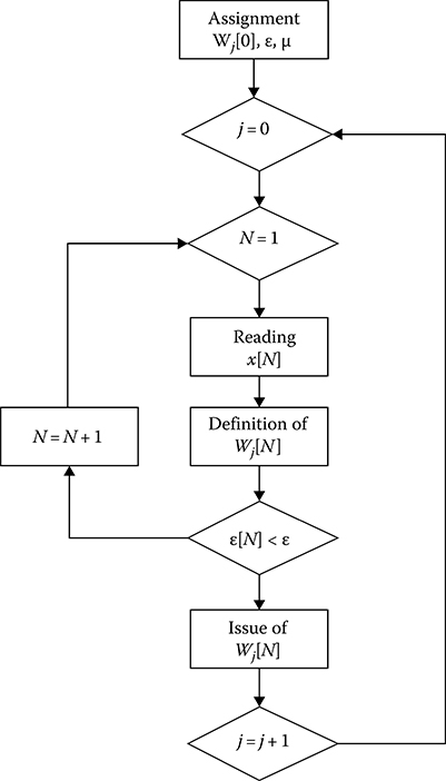
FIGURE 12.19 Block diagram of algorithm for determination of the weight coefficients of adaptive filters.

is the radial frequency of the first harmonic. In addition, we assume that the sampling interval T_s is chosen in such a way that the sample readings x_i are uncorrelated between each other. Taking into consideration the orthogonality between components of the mathematical expectation and a definition of the covariance function (the ambiguity function) of the deterministic signal with constant component as

$C_{E} (k) = \lim_{k \to \infty} \frac{1}{2 k} \sum_{i = - k}^{k} E (κ) E (κ + k), (12.362)$

the covariance matrix elements given by (12.358) can be written in the following form:

$C (k) = σ^{2} σ (k) + \sum_{μ = 0}^{M} A_{μ}^{2} \cos (k ω μ), (12.363)$

where δ(k) is the discrete analog of the Dirac delta function given by (12.170);

$A_{0}^{2} = a_{0}^{2}; (12.364)$

$A_{μ}^{2} = \frac{1}{2} (a_{μ}^{2} + b_{μ}^{2}), μ = 1, 2, \dots, M . (12.365)$

Substituting (12.363) into (12.358), we obtain

$\sum_{j = 0}^{P - 1} {σ^{2} δ (l - j) + \sum_{μ = 1}^{M} A_{μ}^{2} \cos [ω μ (l - j)]} W_{j} = \sum_{μ = 0}^{M} A_{μ}^{2} \cos [ω μ (l - d)] . (12.366)$

Denoting

${\begin{array}{l} φ_{μ} = \sum_{j = 0}^{P - 1} W_{j} \cos (j ω μ); \\ ψ_{μ} = \sum_{j = 0}^{P - 1} W_{j} \sin (j ω μ), \end{array} (12.367)$

we obtain a solution for the weight coefficient W_j in the case of stationary mode in the following form:

$W_{j} = \frac{1}{σ^{2}} \sum_{μ = 0}^{M} A_{μ}^{2} {[\cos (d ω μ) - φ_{μ}] \cos (j ω μ) - [\sin (d ω μ) - ψ_{μ}] \sin (j ω μ)} . (12.368)$

Substituting (12.368) into (12.366), we obtain the system of equations with respect to the unknown variables φ_μ and ψ_μ in the following form:

$φ_{χ} = \frac{1}{σ^{2}} \sum_{μ = 0}^{M} A_{μ}^{2} {[\cos (d ω μ) - φ_{μ}] α_{μ χ} - [\sin (d ω μ) - ψ_{μ}] γ_{μ χ}}; (12.369)$

$ψ_{χ} = \frac{1}{σ^{2}} \sum_{μ = 0}^{M} A_{μ}^{2} {[\cos (d ω μ) - φ_{μ}] β_{μ χ} - [\sin (d ω μ) - ψ_{μ}] ϑ_{μ χ}}; (12.370)$

$χ = 0, 1, \dots, M . (12.371)$

where

$α_{μ χ} = \sum_{j = 0}^{P - 1} \cos (j ω μ) \cos (j ω χ); (12.372)$

$β_{μ χ} = \sum_{j = 0}^{P - 1} \cos (j ω μ) \sin (j ω χ); (12.373)$

$γ_{μ χ} = \sum_{j = 0}^{P - 1} \sin (j ω μ) \cos (j ω χ); (12.374)$

$ϑ_{μ χ} = \sum_{j = 0}^{P - 1} \sin (j ω μ) \sin (j ω χ) . (12.375)$

With the purpose of subsequent simplifying, we are limited by the case when the number of channels N is sufficiently high and in (12.372) through (12.375) we can use the integrals. Moreover, we assume that the constant component of the estimated mathematical expectation is equal to zero, that is, a₀ = 0. As a result of limiting process, we have

${\begin{array}{l} α_{μ χ} = ϑ_{μ χ} = 0.5 P δ (μ - χ); \\ γ_{μ χ} = β_{μ χ} = 0. \end{array} (12.376)$

Using the approximation given by (12.376), the solutions of the equation system given by (12.369) and (12.370) take the following form:

${\begin{array}{l} φ_{μ} = \frac{\cos (d ω μ)}{1 + \frac{2 σ^{2}}{P A_{μ}^{2}}}; \\ ψ_{μ} = \frac{\sin (d ω μ)}{1 + \frac{2 σ^{2}}{P A_{μ}^{2}}} . \end{array} (12.377)$

In the case of stationary mode and high number of channels, the weight coefficients given by (12.368) can be presented in the following form:

$W_{j} = \sum_{μ = 1}^{M} \frac{2 A_{μ}^{2}}{2 σ^{2} + A_{μ}^{2} P} \cos [ω μ (d + j)] . (12.378)$

If the following condition is satisfied

$P ≫ \frac{2 σ^{2}}{A_{μ}^{2}}, (12.379)$

we obtain

$W_{j} = \frac{2}{P} \sum_{μ = 1}^{M} \cos ω μ (d + j) = \frac{2}{P} \times \frac{\sin \frac{π (M + 1) (d + j)}{2 M} \cos \frac{π (d + j)}{2}}{\sin \frac{π (d + j)}{2 M}} . (12.380)$

As we can see from (12.380), the adaptive filter transfer characteristic in the stationary mode will be a sequence of maxima with magnitudes.2M/P and period 2M.

Consider the statistical characteristics of discrete magnitudes of the mathematical expectation estimate $E_{i}^{*}$ at the adaptive filter output in the stationary mode. The mathematical expectation of estimate $E_{i}^{*}$ is defined as

$〈 E_{i}^{*} 〉 = \sum_{j = 0}^{N - 1} W_{j} E_{i - j - d} . (12.381)$

Changing E_i and W_i on their magnitudes from (12.360) and neglecting the sum of fast oscillating terms, we obtain

$〈 E_{i}^{*} 〉 = 0.5 P \sum_{μ = 1}^{M} \frac{1}{q_{μ}^{- 1} + 0.5 P} [a_{μ} \cos (i ω μ) + b_{μ} \sin (i ω μ)], (12.382)$

where

$q_{μ} = \frac{a_{μ}^{2} + b_{μ}^{2}}{2 σ^{2}} (12.383)$

is the SNR for the |LLth component (or harmonic) of the mathematical expectation. As we can see from (12.383), as the number of channels P tends to approach infinity, that is, P → ∞, the mathematical expectation estimate is unbiased.

By analogy, determining the second central moment that is defined completely by the centralized component of stochastic process, it is easy to define the variance of estimate

$Var {E_{i}^{*}} = σ^{2} \sum_{j = 0}^{P - 1} W_{j}^{2} . (12.384)$

We can see from (12.384) that the variance of the investigated mathematical expectation estimate $E_{i}^{*}$ decreases concomitant to a decrease in the number of harmonics M in the observed stochastic process. In the limiting case, given the high number of channels (P → ∞) the variance of the mathematical expectation estimate tends to approach zero in stationary mode; that is, the considered estimate of the periodically changing mathematical expectation $E_{i}^{*}$ is consistent.

To illustrate the obtained results, a simulation of the described adaptation algorithm based on the example of the mathematical expectation estimate E(t) = acos(ωt) given in the form of readings E_i and when the period T₀ corresponds to four sampling periods, that is, T₀ = 4T_s, is carried out. As the centralized component x_{0_i} of stochastic process realization, the uncorrelated samples of Gaussian stochastic process are used. To obtain the uncorrelated samples in the main and reference channels, the delay corresponding to one sampling period (d = 1) is introduced. Initial magnitudes of the weight coefficients, except for the channel with j = 0, are chosen equal to zero. The initial magnitude of the weight coefficient at j = 0 is taken equal to unit, that is, W₀ [0] = 1.

The memory of microprocessor system continuously updates the discrete sample x_i = x_{0_i} + E_i and in accordance with the algorithm given by (12.357) a tuning of the weight coefficients is carried out. The tuning is considered to be complete when the components of the vector differ from each other by no more than 10% on two neighboring steps of adaptation. Thus, the realization formed at the output of adaptive interference and noise canceller is investigated.

The normalized variance of estimate of the harmonic component amplitude, that is, Var{a*}/a², at the SNR equal to unit, that is, q = 1, as a function of the number of adaptation cycles N and two values of the number of parallel channels (P = 4; P = 16) is depicted in Figure 12.20. The dashed lines correspond to the theoretical asymptotical values of variance of the mathematical expectation estimate computed according to (12.378) and (12.384). As we can see from Figure 12.20, the adaptation process is evident and its beginning depends on the number of parallel channels of the adaptive filter.

Images

FIGURE 12.20 The normalized variance of amplitude estimation as a function of the adaptation cycles number.

12.11 Summary and Discussion

Let us summarize briefy the main results discussed in this chapter.

In spite of the fact that the formulaes for the mathematical expectation estimate (12.41) and (12.42) are optimal in the case of Gaussian stochastic process, these formulae are also optimal for the stochastic process that is different from the Gaussian pdf in the class of linear estimations. Equations 12.38 and 12.39 are true if the a priori interval of changes of the mathematical expectation is not limited. Equation 12.38 allows us to define the optimal device structure to estimate the mathematical expectation of stochastic process (Figure 12.1). The main function is the linear integration of the received realization x(t) with the weight υ(t) that is defined based on the integral equation (12.8). The decision device issues the output process at the instant t = T. To obtain the current value of the mathematical expectation estimate, the limits of integration in (12.38) must bet − T and t, respectively, then the parameter estimation is given by (12.43).

The mathematical expectation estimate of the maximum likelihood of stochastic process is both the conditionally and unconditionally unbiased estimate. Conditional variance of the mathematical expectation estimate can be presented by (12.47), from which we can see that the variance of estimate is unconditional. Since, according to (12.38), the integration of Gaussian stochastic process is a linear operation, the estimate E_E is subjected to Gaussian distribution.

The procedure to define the optimal estimate of mathematical expectation of stationary stochastic process is presented in Figure 12.1 in the case of the limited a priori domain of definition of the mathematical expectation. In this case, the maximum likelihood estimate of the mathematical expectation of stochastic process is conditionally biased. The unconditional estimate is unbiased and the unconditional dispersion is given by (12.76).

The Bayesian estimate of the mathematical expectation of stochastic process is a function of the SNR. At low SNR, the conditional estimate bias coincides with the approximation given by (12.82). We can see that the unconditional estimate of mathematical expectation averaged with respect to all possible values E₀ is unbiased. At high SNR, the Bayesian estimate of the mathematical expectation of stochastic process coincides with the maximum likelihood estimate of the same parameter.

Optimal methods to estimate the mathematical expectation of stochastic process envisage the need for accurate and complete knowledge of other statistical characteristics of the considered stochastic process. For this reason, as a rule, various nonoptimal procedures are used in practice. In doing so, the weight function is selected in such a way that the variance of estimate tends to approach asymptotically the variance of the optimal estimate. If the integration time of ideal integrator is sufficiently large in comparison with the correlation interval of stochastic process, then to determine the variance of mathematical expectation estimate of stochastic process there is a need to know only the values of variance and the ratio between the observation interval and correlation interval. The variance of the mathematical expectation estimate of stochastic process is proportional to the spectral density value of fuctuation component of the considered stochastic process at ω = 0 when the ideal integrator is used as a smoothing circuit. In other words, in the considered case, the variance of the mathematical expectation estimate of stochastic process is defined by the spectral components in the case of zero frequency. To obtain the current value of the mathematical expectation estimate and to investigate the realization of stochastic process within the limits of large interval of observation, we use the estimate given by (12.124). Evidently, this estimate has the same statistical characteristics as the estimate defined by (12.111). The previously discussed procedures that measure the mathematical expectation suppose that there are no limitations due to instantaneous values of the considered stochastic process in the course of measurement. Presence of limitations leads to additional errors while measuring the mathematical expectation of stochastic process.

The variance of the mathematical expectation estimate is defined by the interval of possible values of the additional stochastic sequence and is independent of the variance of the observed stochastic process and is forever more than the variance of the equidistributed estimate of the mathematical expectation by independent samples. For example, if the observed stochastic sequence subjected to the uniform pdf coinciding in the limiting case with (12.218), then the variance of the mathematical expectation for the considered procedure is defined by (12.226) and the variance of the mathematical expectation in the case of equidistributed estimate of the mathematical expectation is given by (12.227), that is, the variance of the mathematical expectation estimate in three times more than the variance of the mathematical expectation in the case of equidistributed estimate of the mathematical expectation under the use of additional stochastic signals in the considered limiting case when the observed and additional random sequences are subjected to the uniform pdf. At other conditions, a difference in variances of the mathematical expectation estimate is higher.

Under the definition of stochastic process quantization effect by amplitude on the estimate of its mathematical expectation, we assume that quantization can be considered as the inertialess nonlinear transformation with the constant quantization step and the number of quantization levels is so high that the quantized stochastic process cannot be outside the limits of staircase characteristic of the transform g(x), the approximate form of which is shown in Figure 12.12. The pdf p(x) of observed stochastic process possessing the mathematical expectation that does not match with the middle between the quantization thresholds x_i and x_i+1 is presented in Figure 12.12 for obviousness. The mathematical expectation of the realization y(t) forming at the output of inertialess element (transducer) with the transform characteristic given by (12.228) when the realization x(t) of the stochastic process ξ(t) excites the input of inertialess element is equal to the mathematical expectation of the mathematical expectation estimate given by (12.229) and is defined by (12.230). In general, the mathematical expectation of estimate 〈E〉 differs from the true value E₀, that is, as a result of quantization we obtain the bias of the mathematical expectation of the mathematical expectation estimate given by (12.231). Since the mathematical expectation and the correlation function of process forming at the transducer output depend on the observed stochastic process pdf, the characteristics of the mathematical expectation estimate of stochastic process quantized by amplitude depend both on the correlation function and on the pdf of observed stochastic process.

In the case of the time-varying mathematical expectation of stochastic process, the problem of definition of the mathematical expectation E(t) of stochastic process ξ(t) by a single realization x (t) within the limits of the interval [0, T] is reduced to an estimation of the coefficients. α_i of the series given by (12.256). In doing so, the bias and dispersion of the mathematical expectation estimate E*(t) of the observed stochastic process caused by measurement errors of the coefficients. α_i are given by (12.259) and (12.260). Statistical characteristics (the bias and dispersion) of the mathematical expectation estimate of stochastic process averaged within the limits of the observation interval are defined by (12.261) and (12.262), respectively. The higher the number of terms under expansion in series in (12.256) used for approximation of the mathematical expectation, the higher at the same conditions the variance of time-varying math-ematical expectation estimate averaged within the limits of the observation interval. In doing so, there is a need to note that in general the number N of series expansion terms essentially increases parallel to an increase in the observation interval [0, T], within the limits of which the approximation is carried out.

Thus, at sufficiently large number of the eigenfunctions in the sum given by (12.256) the average time-varying mathematical expectation estimate E (t) is equal to the variance of the initial stochastic process. In doing so, the estimate bias caused by the finite number of terms in series given by (12.256) tends to approach zero. However, in practice, there is a need to choose the number of terms in series given by (12.256) in such a way that a dispersion of the time-varying mathematical expectation estimate caused both by the bias and by the estimate variance would be minimal.

Under definition of estimation of the time-varying mathematical expectation of stochastic process by a single realization, we meet difficulties caused by the definition of optimal time of averaging (integration) or the time constant of smoothing filter at the filter impulse response given before. In doing so, two conflicting requirements arise. On one hand, there is a need to decrease the variance of estimate caused by finite time interval of measuring; this time interval must be large. On the other hand, for better distinguishing the mathematical expectation variations in time, there is a need to choose the integration time to be as short as possible. Evidently, there is an optimal averaging time or the bandwidth of the smoothing filter under the given impulse response, which corresponds to minimal dispersion of the mathematical expectation estimate of stochastic process caused by the factors listed previously.

In practice, the nonstationary stochastic processes with time-varying mathematical expectation or variance or both of them simultaneously are widely used. In doing so, the mathematical expectation and variance vary slowly in comparison with variations of investigated stochastic process. In other words, the mathematical expectation and variance of stochastic process are constant within the limits of the correlation interval. In this case, to define the variance of the time-varying mathe-matical expectation estimate we can assume that the centralized stochastic process ξ₀(t) = ξ(t) − E (t) is the stationary stochastic process within the limits of the interval t₀ ± 0.5T with the correlation function given by (12.317).

In some applications, we can suppose that the time-varying mathematical expectation of stochas-tic process is the periodic function and the value of the period is unknown. At the same time, in a practical case, when the period is much longer than the correlation interval of the observed stochas-tic process is of interest to us. We employ the adaptive filtering methods widely used in practice under interference cancellation to measure. We consider the discrete sample that can be presented in the form discussed in (12.168). The estimated mathematical expectation is the periodical function and can be approximated by the Fourier series with finite number of terms. We can assume that the sampling interval is chosen in such a way that the sample readings remain uncorrelated with each other. Taking into consideration the orthogonality between the components of mathematical expectation and a definition of the covariance function (the ambiguity function) of the deterministic signal with constant component given by (12.362), the covariance matrix elements given by (12.358) can be presented in the form (12.363).

References

1. Lindsey, J.K. 2004. Statistical Analysis of Stochastic Processes in Time. Cambridge, U.K.: Cambridge University Press.

2. Ruggeri, F. 2011. Bayesian Analysis of Stochastic Process Models. New York: Wiley & Sons, Inc.

3. Van Trees, H. 2001. Detection, Modulation, and Estimation Theory. Part 1. New York: Wiley & Sons, Inc.

4. Taniguchi, M. 2000. Asymptotic Theory of Statistical Inference for Time Series. New York: Springer + Business Media, Inc.

5. Franceschetti, M. 2008. Random Networks for Communication: From Physics to Information Systems. Cambridge, U.K.: Cambridge University Press.

6. Le Cam, L. 1986. Asymptotic Methods in Statistical Decision Theory. New York: Springer + Business Media, Inc.

7. Anirban DasGupta. 2008. Asymptotic Theory of Statistics and Probability. New York: Springer + Business Media, Inc.

8. Berger, J. 1985. Statistical Decision Theory and Bayesian Analysis. New York: Springer + Business Media, Inc.

9. Le Cam, L. and G.L. Yang. 2000. Asymptotics in Statistics: Some Basic Concepts. New York: Springer + Business Media, Inc.

10. Liese, F. and K.J. Miescke. 2008. Statistical Decision Theory: Estimation, Testing, and Selection. New York: Springer + Business Media, Inc.

11. Schervish, M. 1996. Theory of Statistics. New York: Springer + Business Media, Inc.

12. Lehmann, E.L. 2005. Testing Statistical Hypothesis, 3rd Edn. New York: Springer + Business Media, Inc.

13. Jesbers, P., Chu, P.T., and A.A. Fettwers. 1962. A new method to compute correlations. IRE Transactions on Information Theory, 8(8): 106–107.

14. Mirskiy, G. Ya. 1972. Hardware Definition of Stochastic Process Characteristics,. 2nd Edn. Moscow, Russia: Energy.

15. Gusak, D., Kukush, A., Kulik, A., Mishura, Y., and A. Pilipenko. 2010. Theory of Stochastic Processes. New York: Springer + Business Media, Inc.

16. Gikhman, I., Skorokhod, A., and S. Kotz. 2004. The Theory of Stochastic Processes I. New York: Springer + Business Media, Inc.

17. Gikhman, I., Skorokhod, A., and S. Kotz. 2004. The Theory of Stochastic Processes II. New York: Springer + Business Media, Inc.

18. Tzypkin, Ya. 1968. Adaptation and Training in Automatic Systems. Moscow, Russia: Nauka.

19. Cox, D.R. and H.D. Miller. 1977. Theory of Stochastic Processes. Boca Raton, FL: CRC Press.

20. Brzezniak, Z. and T. Zastawniak. 2004. Basic Stochastic Processes. New York: Springer + Business Media, Inc.

21. Ganesan, S. 2009. Model Based Design of Adaptive Noise Cancellation. New York: VDM Verlag, Inc.

22. Zeidler, J.R., Satorius, E.H., Charies, D.M., and H.T. Wexler. 1978. Adaptive enhancement of multiple sinusoids in uncorrelated noise. IEEE Transactions on Acoustics, Speech, and Signal Processing, 26(3): 240–254.

..................Content has been hidden....................

You can't read the all page of ebook, please click here login for view all page.

Table of Contents for
Chapter 12 Estimation of Mathematical Expectation

12 Estimation of Mathematical Expectation

12.1 Conditional Functional

12.2 Maximum Likelihood Estimate of Mathematical Expectation

12.3 Bayesian Estimate of Mathematical Expectation: Quadratic Loss Function

12.3.1 LOW SIGNAL-TO-NOISE RATIO (ρ² ≪ 1)

12.3.2 HIGH SIGNAL-TO-NOISE RATIO (ρ² ≫ 1)

12.4 Applied Approaches to Estimate the Mathematical Expectation

12.5 Estimate of Mathematical Expectation at Stochastic Process Sampling

12.6 Mathematical Expectation Estimate Under Stochastic Process Amplitude Quantization

12.7 Optimal Estimate of Varying Mathematical Expectation of Gaussian Stochastic Process

12.8 Varying Mathematical Expectation Estimate Under Stochastic Process Averaging in Time

12.9 Estimate of Mathematical Expectation by Iterative Methods

12.10 Estimate of Mathematical Expectation with Unknown Period

12.11 Summary and Discussion

References

Table of Contents for Chapter 12 Estimation of Mathematical Expectation

Create new playlist

Sign In

Sign Up

Table of Contents for
Chapter 12 Estimation of Mathematical Expectation