
10 Global Digital Signal Processing System Analysis
10.1 Digital Signal Processing System Design
10.1.1 STRUCTURE OF DIGITAL SIGNAL PROCESSING SYSTEM
We consider the following problem—to design and construct a complex radar system (CRS) based on the all-round surveillance radar with the uniform antenna rotation. The main task of this CRS is to search for all the detected targets, to integrate information, and to make a generalization of the air situation. An additional task is target tracking with the high accuracy of important targets from a user viewpoint. In this case, the following version of a global digital signal processing system structure may be used to design and construct the CRS based on the all-round surveillance radar with the uniform antenna rotation (see Figure 10.1) [1, 2].
Detection and tracking of all targets in an all-round surveillance radar coverage with accuracy that is sufficient to reproduce and estimate data of the air situation are carried out by the so-called rough channel of a global digital signal processing system covering the whole scanned area. The rough channel consists of the following subsystems: the binary signal quantization, the specific microprocessor network for target return signal preprocessing, and the microprocessor network for digital signal reprocessing and control. Employment of binary quantization and simplified versions of digital signal processing algorithms allows us to implement the microprocessor networks and sets in this channel of global digital signal processing system of the all-round surveillance radar with the uniform antenna rotation.
Accurate tracking of the targets that are important from a user viewpoint is carried out by radar measurers. The radar measurer is the digital device assigned to solve the signal processing problems for one or several targets. The process of accurate target tracking can be organized at least by two ways:
An individual radar measurer is assigned for each target and it is capable of target tracking within the period when the target is within the limits of radar coverage. These radar measurers are constructed by the principle of automatic tracking systems and are called moving target indicators (MTIs). The MTI number corresponds to the number of targets subjected to tracking, i e., NMTI = Ntg. In this case, we have the digital signal processing system with computational parallelism by a set of objects subjected to processing (see Chapter 7).
The MTI system operates based on the main principles of queuing theory. The time sequence of signals received by each target tracking gates is considered as a request queue. In doing so, the targets subjected to tracking can be served by the lesser number of nontracking at the present time MTI, i e., NMTI < Ntg. Interaction between the rough and “accurate” channels of global digital signal processing system can be organized in the following form. All targets are checked based on their importance by the queuing system using the digital signal reprocessing microprocessor network. The coordinates of center and dimensions of the preliminary target lock-in gate are sent to the device of physical gating by targets, an important criterion of which exceeds the given threshold and trajectory parameters of the target subjected to accurate tracking are sent to the dispatch device of MTI system simultaneously. Under scanning of the corresponding direction, the device of physical gating organizes a selection of signals of the gated area of radar coverage. The target return signals received by gates after an analog-to-digital converter (ADC) come in at the input of MTI selected by the dispatch device and are processed by MTI. Initial values of target trajectory parameters determined by the digital signal reprocessing microprocessor network are used by MTI at the first stage of accurate definition of the target trajectory parameters. Furthermore, the extrapolated coordinates of gate centers and dimensions are computed and are sent to the device of physical gating by corresponding MTI networks. Under unspecified reset action of target trajectory tracked by MTI, the target relock-in is carried out using the global digital signal processing system rough channel. The considered structure of the global digital signal processing system possesses a high reliability and requires moderate designing charges and operating costs.
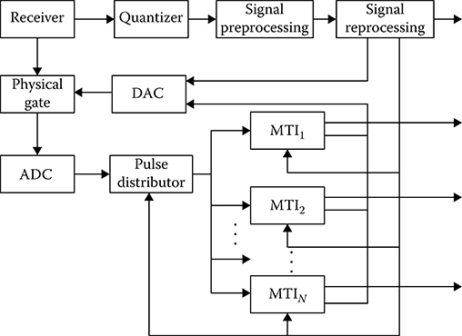
FIGURE 10.1 Global digital signal processing system structure.
10.1.2 STRUCTURE AND OPERATION OF NONTRACKING MTI
Let us consider the nontracking MTI system. The nontracking MTI is the microprocessor network for digital signal processing. The signals come in at the nontracking MTI input from the radar coverage zone limited by the physical gate. The nontracking MTI structure is shown in Figure 10.2, which shows that the nontracking MTI possesses the same functions as those under the target tracking. The essential difference is matching the signal preprocessing operations with a selection of target pips in the target tracking gate. In doing so, owing to limiting gate dimensions it is possible to realize the signal quantization and signal processing algorithms. As to the target trajectory parameter smoothing operations, the nontracking MTI ensures the maneuvering of target tracking.
Consider in detail the signal preprocessing and selection in the target tracking gate algorithm. The problems of target detection, definition of target position, and selection of target return signals within the limits of gate are reduced to checking several hypotheses. Moreover, a signal absence in the gate is considered as the hypothesis ℋ0, and the alternative hypotheses are the hypotheses about the signal presence in a single (or several) gate cell. We consider the gate cell as the gate volume (or square) element limited by sampling intervals on the radar range, azimuth, and tilt angle coordinates. An optimal procedure under processing the observation results with the purpose of checking the statistical hypotheses is a generation of the likelihood ratio and its comparison with the threshold that is selected from acceptable losses attributed to correct or incorrect decisions. Furthermore, we consider the signal processing algorithm of binary signals in two-dimensional gate, as an example. Under optimal binary signal processing within the limits of two-dimensional (by radar range and azimuth) gate, the logarithm of likelihood ratio takes the form [3]
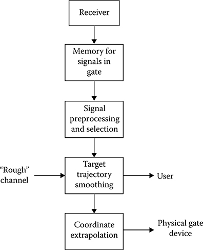
FIGURE 10.2 Nontracking MTI structure.
where
dij are the values of binary signals, “1” or “0,” in ijth gate cell; i = 1,…, n and j = 1,…, m are the number of discrete gate elements by the radar range and azimuth, respectively
ϖ(ij|i0j0) is a set of the weight coefficients, with which the signals 1 and 0 are added in the gate cells under formation of the likelihood ratio
The concrete form of the function ϖ(ij|i0j0) depends on the shape of amplitude envelope of two-dimensional signal that is processed. If we consider the signal model in the form of two-dimensional pdf surface in the polar coordinate system, the coordinates r and β, the weighting function takes the following form:
where
C1 and C2 are the constant values
Δr and Δβ are the gate sampling intervals by the coordinates r and β
δr and δβ are the half signal bandwidth by the coordinates r and β at the level exp (−0.5)
i0 and j0 are the coordinates of the maximal signal amplitude envelope
The two-dimensional likelihood ratio surface, which is the initial likelihood ratio to detect and select the target return signal pips within the limits of gate, is obtained as a weighting the binary target return signals by the weight function (10.2). Moreover, in this case, the two-dimensional likelihood ratio surface peaks contain all information about the signal presence and signal coordinates.
The detection and selection problem of a single target within the limits of the gate is assigned in the following way based on information contained in the likelihood ratio maxima. First, we take the hypothesis that there is only a single target within the limits of the gate. In the considered case, the event, when several targets are within the limits of the gate, is possible but is improbable. Using the relief of the two-dimensional likelihood ratio surface with M peaks of different heights, there is a need to define the maximum (the peak) formed by the target return signal and, if a “yes,” there is a need to define the coordinates of this two-dimensional likelihood ratio surface maximum. The amplitudes of peaks Zl(l = 1, 2,…,M) and their coordinates ξl and ηl with respect to the gate center are used as the input parameters, based on which the decision is made. If the hypothesis about the statistical independence of the two-dimensional likelihood ratio surface peak amplitudes is true and the coordinates of the two-dimensional likelihood ratio surface maxima are known within the limits of range where the target return signal is present, the optimal detection–selection problem of the target return signal pips within the limits of gate is solved in two steps [4].
Step 1: There is a need to select the two-dimensional likelihood ratio surface maximum with the number l* with quadratic form
where
is the average amplitude of the two-dimensional likelihood ratio surface in the signal domain
is the amplitude variance of the two-dimensional likelihood ratio surface in the signal domain
Step 2: Compare the obtained quadratic form Ql* with the threshold defined based on the accept-able probability of error decisions and, in the case of exceeding the threshold, issue a decision about the target pip detection. The coordinates of the two-dimensional likelihood ratio surface maximum are considered as the coordinates of the detected target pip within the limits of gate.
The described optimal algorithm is difficult to realize in practice owing to the high work content to estimate the average value of amplitude and amplitude variance of the two-dimensional likelihood ratio surface in the signal domain. Therefore, the following simplified algorithms of target pip detection and selection are used in practice:
Algorithm of detection and selection using the two-dimensional likelihood ratio surface maximum—at first, there is a need to define the amplitude of the two-dimensional likeli-hood ratio surface maximum within the limits of gate and compare with the threshold. Target detection pip is fixed if the amplitude of the two-dimensional likelihood ratio surface maximum exceeds the threshold and the coordinates are defined by a position of the two-dimensional likelihood ratio surface maximum within the limits of gate.
Algorithm of detection and selection using the two-dimensional likelihood ratio surface maximum amplitude exceeding the threshold and possessing a minimal deviation with respect to the gate center.
The first algorithm possesses the best selecting features evaluated by the probability of detection PD and selection at the fixed probability of false alarm PF. For each case, there is a need to carry out a detailed analysis and find the trade-off, taking into consideration the requirements of the problem solution quality and available computational resources with the purpose of selecting the accept-able signal detection and selection algorithms within the limits of the target tracking gate of the nontracking MTI.
10.1.3 MTI AS QUEUING SYSTEM
Each MTI consists of the following blocks solving their own functions (see Figures 10.3 through 10.5):
Static memory of the digital target return signals within the limits of physical target tracking gate
Detector-selector assigned to detect and select the target return signals within the limits of physical target tracking gate
Measurer assigned to estimate the target trajectory parameters, to extrapolate the target trajectory coordinates, and to compute dimensions of physical target tracking gate
Static memory can be realized in the matrix form (the two-dimensional case) or as a set of matrices (under the target return signal processing within the limits of three-dimensional physical target tracking gate) of memory cells. Each memory cell stores information obtained as a result of the target return signal sampling within the limits of the corresponding volume or area element of the physical target tracking gate. Processing of information about the target return signals stored by the memory is carried out after flling all physical target tracking gate cells. After processing of the stored information about the target return signals, the corresponding memory matrix is ready to receive new information. One or several specific microprocessor networks can be used as the detector-selector. Taking into consideration the large computation content under realization of signal processing algorithms to estimate the target trajectory parameters and coordinates in the course of the target return signal reprocessing and, additionally, the necessity to store previous information about each target tracked trajectory, it is worth constructing the MTI based on a set of microprocessor networks.
Under the target tracking by several MTIs, we are able to reduce a set of blocks owing to an efficient structural organization. Now, consider the following versions:
System “n − 1 − 1” (see Figure 10.3). The memory is the n-channel queuing system with losses and the detector-selector and MTI are the one-channel queuing systems with request queue waiting; the system n − 1 − 1 is the three-phase queuing system with input failures.
System “n − n − 1” (see Figure 10.4). This system is different from the previous one in that each detector-selector has own memory and the “memory-detector-selector” devices connected in series can be considered as a single queuing system channel. The totality of the memory-detector-selector devices is the n-channel queuing system with losses. The MTI, as earlier, is considered as the one-channel queuing system with request queue waiting.
System “n − m − 1” (see Figure 10.5). For this system, the queuing request forming at the n-channel memory output comes in at the m-channel detector-selector passing a splitter. Generally, the splitter operates as the associate device or probabilistic automation unit, a mode of which is defined by characteristics and parameters of the output request queue incoming from the memory and by a mode of the second device. The second device is the m-channel queuing system with request queue waiting. The data forming at the second device output come in at the input of the third device, which is the one-channel queuing system with request queue waiting.

FIGURE 10.3 Nontracking MTI blocks organizing the system “n–1–1”

FIGURE 10.4 Nontracking MTI blocks organizing the system “n–n–1”

FIGURE 10.5 Nontracking MTI blocks organizing the system “n–m–1”
All considered and discussed versions of target tracking by several MTI systems are the three-phase queuing systems. Each phase is represented by one or several devices of the queuing system connected in series. In a general case, the request queuing time for each device is the random variable with pdf available to investigate and define. It is assumed that there is a simple request queue at the first-phase input of the queuing system. The request queue coming in at the first device input is immediately served if, at least, one channel of the queuing system is free from service; otherwise, the request is rejected and flushed. The requests carried out by the first device are processed sequentially at the next phases, in other words, the request loss at each next phase or stage is inadmissible. In line with this, the memory device with the purpose of storing requests in line should be provided before the second and third phases of the queuing system.
Now, let us discuss the pdf of request queuing time at different phases of the queuing system. The request queuing time for memory device is the time to fll out the memory cells within the limits of the physical target tracking gate, which can be presented in the following form:
where
Δβgate is the angular size by azimuth in radian
Tscan is the scanning period
Dimensions of the physical target tracking gate are determined based on the required probability of target pip hitting within the limits of gate taking into consideration the random errors in the course of target trajectory coordinate measurement, random error of coordinate extrapolation, and dynamical errors caused by maneuvering targets. Errors of measurements and extrapolation by each individual coordinate are subjected to the normal Gaussian pdf with zero mean and known variance.
As noted in Chapter 4, under stable target tracking, the physical target tracking gate dimensions by each coordinate are minimal, i e., ΔZmin {Z = {r, β}}. The target maneuver, regular and random deviations of target return signal power, and misses of target pips on target trajectory track lead to an increase in the physical target tracking gate dimensions in comparison with minimal ones. At the same time, the probability of event that the physical target tracking gate dimensions are minimal or close to minimal is the highest. Distribution corresponding to described process of changes in dimensions of the physical target tracking gate can be presented in the following form:
where is the variance of changes in the physical target tracking gate dimensions by the coordinate Z. In this case, the pdf of request queuing time takes the following form:
Sometimes the physical target tracking gate dimensions are chosen as constant values determined at the maximum total error of extrapolation. For this case, the request queuing time by memory will be constant.
When the simplest signal processing algorithm for definition of the maximal weighted sum of the target return signals is used in the detector–selector, the signal processing operations are the following:
Definition of the weighted sum amplitude of the target return signals for each physical target tracking gate cell
Sequential comparison of amplitudes of the target return signals for each physical target tracking gate cell with the purpose of choosing the maximum one
Comparison of selected amplitudes of the target return signals for each physical target tracking gate cell with the threshold and making a decision about detection of the target pip within the limits of the physical target tracking gate
In this case, the analysis time is defined by dimensions of the physical target tracking gate. Furthermore, we consider the case of two-dimensional physical target tracking gate. According to (10.5), the dis-tribution of normalized dimensions of the two-dimensional physical target tracking gate by each coordinate is defined as
where
In this case, the pdf of two-dimensional physical target tracking gate area Sgate is defined as the pdf of product between the random variables x and y with the pdf given by (10.7) and (10.8), respectively. The cumulative probability distribution function of the two-dimensional physical target tracking gate area Sgate is given by
Differentiating (10.10) by Sgate, we obtain the pdf in the following form:
Equation 10.11 is not integrated in an explicit form. Results of numerical integration show that at small values of S0 the pdf of Sgate can be approximated by exponential pdf with the shift given by the following form:
Under increasing S0, the pdf of the two-dimensional physical target tracking gate area Sgate is approximated by the truncated normal Gaussian pdf:
In accordance with (10.12) and (10.13), the pdf of request queuing time in the detector–selector can also be approximated either by the truncated exponential pdf with the shift in the following form:
where μ is the intensity of request queuing by the detector–selector or by the truncated and shifted normal Gaussian pdf given by
Since generally, the exact definition of the request queuing time pdf is impossible, we use two types of approximation given by (10.14) and (10.15) in further analysis of the detector–selectors. Finally, in the considered case we think that the time required to complete all signal processing operations is a constant value.
Now, consider and discuss the quality of service (QoS) of the multiphase queuing system. We can think that QoS is based on the probability of failure under a service of the next request as a function of input memory capacity and the average time of request processing by the queuing system:
where
is the average request queuing time during the ith phase
is the average waiting time for request queue before the ith phase or stage
Taking into consideration these QoS indicators under the known number of operations that are required for a single request queuing, we can define and estimate the required speed of microprocessor network operation realizing each phase of queuing systems.
Difficulties under analysis of multiphase queuing systems are the following. At all cases of practical importance, the output stream of phase takes more complex form in comparison with the incoming request queue. In some cases, the output request queue can be approximated by the simplest incoming stream with the same parameters. Then we can use analytical procedures and methods of the queuing theory to analyze the next phase or stage. If this approximation is impossible, then the only method to investigate the stream is the simulation. Rational combination of analytical and simulation methods and procedures allows us to solve the problem of the three-phase signal processing system analysis using the MTI system for any design and construction version.
10.2 Analysis of ”n–1–1” MTI System
10.2.1 REQUIRED NUMBER OF MEMORY CHANNELS
Since according to the operational conditions of MTI system the digital signal processing within the limits of the physical target tracking gate can be started only after flling out all memory cells of this gate, the request queuing time in memory is equal to the time of scanned angle by radar antenna corresponding to the azimuth dimension of the physical target tracking gate. This time is distributed according to (10.6). In this case, the average memory request queuing time is given by
The acceptable probability of request losses in memory is given and equal to, as a rule, Ploss = 10−3 − 10−4. It is assumed that the request queue at the memory input is the simplest with the densityγin that is given. The density γin is assigned based on the possible number of targets liable to tracking.
Using the Erlang formula [4]
we can determine the required number of channels N (gates). The output request queue can be considered as an iteration of the input request queue, i e., the simplest at the low probability of failure.
10.2.2 PERFORMANCE ANALYSIS OF DETECTOR—SELECTOR
QoS factors of the detector–selector as the one-channel queuing system are the average request queuing time and the average waiting time for service . At first, consider the case of the exponential with shift pdf for . In this case,
where στDS = μ−1. The variance of request queuing time is determined in the following form:
Denote . Then, we obtain
Under the unpriority queuing, the average waiting time is given by
Substituting (10.22) into (10.23), we obtain
Expressing τ0 over based on (10.21), after elementary algebra we obtain
Denoting , we obtain finally
wait
χDS is the loading factor of the detector-selector
Formula (10.26) allows us to determine the detector-selector QoS factors as a function of its loading and relative shift ν of the pdf.
If the request queuing time τDS is distributed according to (10.15), then
Taking into consideration that and , we obtain
The average waiting time is determined as
or
Formula (10.32) allows us to determine also the detector–selector performance at the corresponding pdf of request queuing time. In particular, (10.26) and (10.32) show that an increase in relative shift of the pdf of request queuing time at the same loading factor χDS leads to a decrease in the average relative waiting time. As ν → ∞, the limiting value of this time tends to approach the value corre-sponding to the constant request queuing time. In this case, the request queue is stored in the input memory device. Computing the memory capacity by (10.30), there is a need to take into consideration the average waiting time for request queue in the detector–selector adding the average request queuing time for queuing requests in the memory device:
Further, knowing the average request queuing time and the number of reduced operations required for a single realization of the target detection and selection algorithm, we are able to deter-mine the effective speed of operation of the detector–selector:
Now, consider the request queue at the detector-selector output taking into consideration that the loading factor χDS is close to unit, i e., χDS = 0.9 ÷ 0.95. The detector–selector output request queue is defined by instants of the request incoming for service, the request queuing time, and the waiting time to start a service. Let t1, t2,…, ti−1, ti, ti+1 be the instants of the request queue incoming at the detector-selector input, be the waiting time for request queue coming in at the instant ti, and τi = τ0 + ξi be the request queue time of the ith request, where τ0 is the constant and ξi is the random component of the request queue time. In the course of service of the request queue, two cases are possible.
First case: The request queue comes in at the instant ti when the detector–selector serves the previous request and stands in a queue (see Figure 10.6a and b). The waiting time to start the given request queue is . Denote the time intervals between two requests at the detector-selector input Δti = ti − ti−1 and output , respectively. Then, in the considered case (Figure 10.6b), the time interval at the detector-selector output between queuing requests is equal to the request queue time:
Second case: The request queue comes in for service at the instant ti+1 when the detector–selector is free and accepts the request queue immediately (Figure 10.6c). In this case, the time interval between two neighboring queuing requests at the detector–selector output is greater than the request queue time interval on the value of downtime Δt:
Since, by the initial condition, the loading factor χDS is high, the probability of the second case is proportional to 1 − χDS and low by magnitude. Therefore, we are able to think that there is a request queue at the detector–selector input, i e., Case 1 is realized with the high probability.

FIGURE 10.6 Time diagram of request queue processed by the detector-selector: (a) service of previous request; (b) the request stands in queue; and (c) the request queue is accepted and processed.
In accordance with the earlier discussion, a distribution of time intervals between the queuing requests served by the detector-selector (the detector-selector input) can coincide with distribution of the request queue time in the detector-selector. The parameter of request queue at the detector-selector output coincides with the parameter of the incoming request queue.
10.2.3 ANALYSIS OF MTI CHARACTERISTICS
The MTI is considered as the one-channel queuing system with waiting time. The request queue served by the detector-selector with the parameter γin and the pdf of time intervals between the requests coinciding with the pdf of request queue time in the detector-selector given by (10.14) and (10.15) comes in at the MTI input. The request queue time in MTI is constant and equal to τMTI = a. Depending on the relation between the constant constituent τ0 in (10.36) and the duration of the request queuing time interval in MTI τMTI = a, the following cases are possible.
Case 1: a ≤ τ0. MTI can forever serve the request queue before the next request queue comes in, and the downtime interval is even possible. The average duration of downtime depends on the variance of the random component ξi of the time interval between the requests at the MTI input. If the pdf of time intervals between the requests coming in at the MTI input is subjected to the exponential pdf with the shift given by (10.14), then the average downtime is defined as
If the pdf of time intervals between the requests coming in at the MTI input is subjected to the pdf given by (10.15), we have
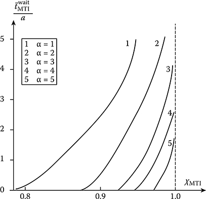
FIGURE 10.7 Relative waiting time versus the loading factor at different values of shift coefficient α.
Case 2: . There is a request queue at the MTI input. It is impossible to compute the request queue length or the waiting time using analytical methods because the input request queue is not simple. To define the mentioned characteristics there is a need to apply a simulation. The greatest difficulty is to simulate the request queue with the pdf given by (10.14) or (10.15). The curves of relative waiting time for request queue by MTI as a function of the loading factor and the shift coefficient as the parameter are shown in Figure 10.7. As we can see from Figure 10.7, the average waiting time at the MTI input under the fixed loading factor is a function of the shift coefficient α. If α ≥ 3, the input request queue degenerates into a regular request queue and the MTI request queue time is approximately equal to τ0. In this case, the request queue at the MTI input is absent and the input register is used as the buffer memory.
10.3 Analysis of “n–n–1” MTI System
The “n–n–1” MTI system is presented in Figure 10.4. For this system the request queuing by the detector-selector is started immediately after flling out the memory matrix. If, as before, we assume that the pdf of time to fll out the memory is given by (10.6), then the pdf of request queuing time by each channel of the system memory-detector-selector is a combination of the pdfs given by (10.6) and (10.14) or (10.6) and (10.15) and the average request queuing time is defined as
where
is the average time to fll out the memory
is the average time for request queuing by the detector-selector given by (10.17) or (10.29)
Now, if the request queuing parameter is given (the input request queuing is considered as the simplest, as before), the number of channels of the system memory-detector-selector can be determined using the Erlang formula (10.18) at the given probability of failure Pfailure.
Let us discuss the request queuing pdf at the output of n-channel system memory-detector-selector. Action of the considered system memory-detector-selector on the incoming request queue can be presented as an expansion of the simplest request queue on the elementary request queues, the number of which is equal to the number of channels of the system memory-detector-selector. In a general case, these elementary request queues may not be the simplest. The output request queue of the system memory-detector-selector is a superposition of elementary request queues and can be considered as the simplest request queue with the parameter equal to the parameter of the incoming or input request queue at low values of Pfailure based on Sevastyanov’s theorem [5]. The request queue time in MTI is constant and equal to a, as earlier. Therefore, the average waiting time for request queue by MTI is defined as
The average number of request in queue is given by
and the variance
where χMTI is the MTI loading factor.
Knowing and , we can define the buffer memory capacity at the MTI input under the given acceptable probability to loss the request and assuming, for example, that the pdf of the number of requests in queue is the normal Gaussian. This approximation makes sense only at high values of . In this case, the probability of losing the request at the MTI input is defied as [6]
where QBM is the required buffer memory. There is a need to note that the acceptable probability of losing the request at the MTI input must be, at least, on the order less than the acceptable probability of losing the request at the system input. Only in this case the main requirement to the system operation will be satisfied, namely, all queue requests that pass the first phase of queue must be served by MTI.
10.4 Analysis of ”n − m − 1” MTI System
The considered system is the three-phase queuing system with losses at the input. The first phase is the n-channel queuing system with losses. Definition of the required number of channels of this system is carried out according to the procedure discussed earlier. The second phase is the m-channel queuing system with waiting. Analysis of QoS factors of this system is the subject of the present section. The input request queue is the simplest one with the parameter γin. We assume that the splitter operates as a counter with respect to the base m sending to the ith channel, i = 1, 2,…, m, the requests with numbers i, i + m, i + 2m. This allocation method of requests is called the cyclic way. The simplest request queue thinned in m − 1 times, ie., the Erlang request queue of the (m − 1)th order, with the following pdf
comes in at the input of each channel of the one-channel queuing system. The condition of the m-channel queuing system stationary mode is the following:
At this time we assume that the average request queue time is the same for all channels. Thus, in the considered case, the one-channel queuing system with the Erlang incoming request queue possessing the pdf equal to γin m−1 and the request queue time subjected to the pdf given by (10.14) and (10.15) with the parameters and is investigated. The result of investigation must be the statistical characteristics of the request queue waiting time, namely, the average time and the variance of this time .
As noted earlier, the analytical investigation of queuing systems with the incoming request queue different from the simplest one is a complicated problem. A general approach to solving this problem is discussed in Ref. [5]. However, an implementation of this general approach to specific conditions of our problem is difficult, not obvious, and does not lead to final formulae for and . The explicit solutions for . obtained by numerical simulation are shown in Figure 10.8, where the solid lines represent the exponential with shift pdf of request queue time and the dashed lines represent the truncated and shifted normal Gaussian pdf. As we can see from Figure 10.8, with an increase in m the relative average waiting time decreases exponentially. The shift coefficient α affects the average waiting time by an analogous way as for previously discussed systems. At the given parameters γin, m, α, we can compute > based on the curves presented in Figure 10.8. We are able to define the average waiting time of request queue and, taking into consideration the average waiting time of request queue, we are able to define the required number of channels n for the first-phase queuing system.

FIGURE 10.8 Average waiting time versus the number of queuing system channels.
Dependences of the required speed of operation for each mth channel of the second-phase queuing system for several values of the input request queue parameter γin as a function of the average number of reduced operations required to process a single request under the loading factor of each mth channel χi = 0.9m are shown in Figure 10.9 for the truncated and shifted normal Gaussian pdf given by (10.15). The required speed of operation is computed by the following formula:
Analysis of (10.47) and dependences in Figure 10.9 show that at the fixed parameters of the input request queue and the already-given number of operations for a single realization of digital signal processing algorithm, the required speed of operation of the second-phase queuing system decreases proportionally to the number of channels in this system.
A set of requests processed by the second-phase queuing system form the incoming request queue for the third-phase queuing system that is a one-channel queuing system with waiting. According to the limiting theorem for summarized flows, the incoming request queue at the third-phase queuing system input is very close to the simplest one with the parameter γin The request queue time in the third-phase queuing system is constant, as earlier. Therefore, a computation of required characteris-tics of the three-phase queuing system and buffer memory capacity is carried out by the procedure discussed in Section 10.3.
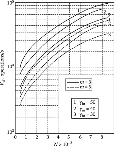
FIGURE 10.9 Required speed of operation for each mth channel of the second-phase queuing system for several values γin versus the average number of operations under the loading factor χi = 0.9m; truncated and shifted normal Gaussian pdf.
10.5 Comparative Analysis of Target Tracking Systems
The total QoS factors of discussed versions of the target tracking systems are the following:
The required number of input memory channels under the given probability of failure Pfailure
The required effective speed of operation
The average time required to process the request by the queuing system
Based on the discussions provided in the previous sections, we are able to compare the considered target tracking systems under the following initial data:
The request queue at the target tracking system input is the simplest with γin = 40 s−1.
The acceptable probability of failure at the target tracking system input Pfailure = 10−3.
The loading factor of the detector-selector and MTI is χDS (MTI) = 0.9.
The pdf of request queue time in the detector-selector is given by (10.15) with α = 2.
The average number of reduced short operations required to process a single request by the detector-selector system is .
The number of reduced short operations required to process a single request by the MTI is .
Scanning by azimuth with the uniform velocity V0 = 250° s−1.
Minimal size of the target tracking gate by azimuth is .
Minimal time to fll out the memory matrix (the constant constituent of the request queue time in memory) .
If we assume in (10.6) , then the average request queue time in the memory is defined as
To compare the target tracking system of various types we define the following:
Number of channels (matrices) of the input memory Nmemory
Average waiting time at the detector–selector input
Average request queue time in the detector–selector
Required speed of operation of the detector–selector
Number of detector–selectors NDS
Average waiting time at the MTI input
Request queue time in MTI τMTI
Number of the buffer memory cells at the MTI input NBM (MTI)
Required speed of MTI operation
Average request delay by queuing system τΣ
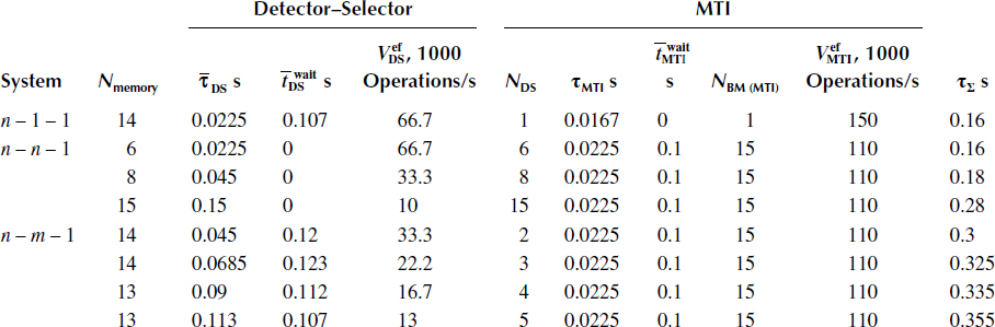
Computational results are presented in Table 10.1, which shows that the system “ n–1–1” ensures the minimal average time of signal processing by one target equal to τΣ = 0.16s at the speed of operation of MTI equal to operations per second and the speed of operation of detector–selector equal to operations per second, i.e., providing a refreshment on nine targets in the course of each scanning. The same average time of signal processing is provided by the system “n–n–1” when there are six detector–selectors with the speed of operation equal to operations per second but at the lesser speed of MTI operation. Obviously, a realization of this version is expensive in comparison with the system “n–1–1”. Other versions of the system can be realized using the detector–selectors with the low speed of operation that can be a clincher in their favor [7]. The system “n–m–1” can also be realized using the detector–selectors with a low speed of operation. In doing so, the number of detector–selectors is not high (two or three), which is an advantage of this system in comparison with the second type of system. The disadvantage is an increase in the request queue time.
Selection of definite version of the system is defined by computational resources and acceptable time of signal processing. Evidently, the most effective system from considered ones is the system. “ n–m–1” with two or three detector–selectors.
TABLE 10.1
Comparative Analysis of Target Tracking Systems
10.6 Summary and Discussion
Detection and tracking of all targets in the all-round surveillance radar coverage with accuracy sufficient to reproduce and estimate data of the air situation are carried out by the so-called rough channel of global digital signal processing system covering the whole scanned area. The rough channel consists of the following subsystems: the binary signal quantization, the specific microprocessor network for target return signal preprocessing, and the microprocessor network for digital signal reprocessing and control. Employment of binary quantization and simplified versions of digital signal processing algorithms allows us to implement the microprocessor networks and sets in this channel of global digital signal processing system of the all-round surveillance radar with the uniform antenna rotation.
The detection and selection problem of a single target within the limits of the gate is assigned in the following way based on information contained in the likelihood ratio maxima. First, we take the hypothesis that there is only a single target within the limits of the gate. In the considered case, the event, when several targets are within the limits of the gate, is possible but it is improbable. Using the relief of the two-dimensional likelihood ratio surface with M peaks of different heights, there is a need to define the maximum (the peak) formed by the target return signal and, if a “yes,” there is a need to define the coordinates of this two-dimensional likelihood ratio surface maximum. The amplitudes of peaks Zl (l = 1, 2,…, M) and their coordinates ξl and ηl with respect to the gate center are used as the input parameters, based on which the decision is made. If the hypothesis about the statistical independence of the two-dimensional likelihood ratio surface peak amplitudes is true and the coordinates of the two-dimensional likelihood ratio surface maxima are known within the limits of range where the target return signal is present, the optimal detection-selection problem of the target return signal pips within the limits of gate is solved in two steps.
All considered and discussed versions of target tracking by several MTI systems are three-phase queuing systems. Each phase is represented by one or several devices of queuing system connected in series. Generally, the request queuing time for each device is the random variable with pdf available to investigate and define. It is assumed that there is a simple request queue at first-phase input of the queuing system. The request queue coming in at the first device input is immediately served if, at least, one channel of the queuing system is free from service; otherwise, the request is rejected and flushed. The requests carried out by the first device are processed sequentially at the next phases; in other words, the request loss at each next phase or stage is inadmissible. In line with this, the memory device with the purpose storing requests in line should be provided before the second and third phases of the queuing system.
Difficulties under analysis of multiphase queuing systems are the following. At all cases of practical importance, the output stream of phase takes a more complex form in comparison with the incoming request queue. In some cases, the output request queue can be approximated by the simplest incoming stream with the same parameters. Then we can use analytical procedures and methods of the queuing theory to analyze the next phase or stage. If this approximation is impossible, then the only method to investigate the stream is the simulation. A rational combination of analytical and simulation methods and procedures allows us to solve the problem of the three-phase signal processing system analysis using the MTI system for any design and construction version.
References
1. Lyons, R.G. 2004. Understanding Digital Signal Processing. 2nd Edn. Upper Saddle River, NJ: Prentice Hall, Inc.
2. Harris, F.J. 2004. Multirate Signal Processing for Communications Systems. Upper Saddle River, NJ: Prentice Hall, Inc.
3. Barton, D.K. 2005. Modern Radar System Analysis. Norwood, MA: Artech. House, Inc.
4. Skolnik, M.I. 2008. Radar Handbook. 3rd Edn. New York: McGraw-Hill, Inc.
5. Gnedenko, V.V. and I.N. Kovalenko. 1966. Introduction to Queueing Theory. Moscow, Russia: Nauka.
6. Skolnik, M.I. 2001. Introduction to Radar Systems. 3rd Edn. New York: McGraw-Hill, Inc.
7. Hall, T.M. and W.W. Shrader. 2007. Statistics of clutter residue in MTI radars with IF limiting, in IEEE Radar Conference, April 2007, Boston, MA, pp. 01–06.