Chapter 15 Estimate of Stochastic Process Frequency-Time Parameters

Search in book...
Toggle Font Controls
Create new playlist

Name your new playlist

Playlist description (optional)
Sign In

Email address

Password

Forgot Password?

or

Continue with Facebook

Continue with Google
Sign Up

Full Name

Email address

Confirm Email Address

Password

or

Continue with Facebook

Continue with Google

Considered parameters of the stochastic process, namely, the mathematical expectation, the variance, the probability distribution and the density functions, do not describe statistic dependence between the values of stochastic process at different instants. We can use the following parameters of the stochastic process, such as the correlation function, spectral density, characteristics of spikes, central frequency of narrowband stochastic process, and others, to describe the statistic dependence subject to specific problem. Let us briefly consider the methods to measure these parameters and define the methodological errors associated, in general, with the finite time of observation and analysis applied to the ergodic stochastic processes with zero mathematical expectation.

As applied to the ergodic stochastic process with zero mathematical expectation, the correlation function can be presented in the following form:

$R (τ) = \lim_{T \to \infty} \frac{1}{T} {\int^{}}_{0}^{T} x (t) x (t - τ) d t . (15.1)$

Since in practice the observation time or integration limits (integration time) are finite, the correlation function estimate under observation of stochastic process realization within the limits of the finite time interval [0, T] can be presented in the following form:

$R^{*} (τ) = \frac{1}{T} {\int^{}}_{0}^{T} x (t) x (t - τ) d t . (15.2)$

As we can see from (15.2), the main operations involved in measuring the correlation function of ergodic stationary process are the realization of fixed delay τ, process multiplication, and integration or averaging of the obtained product. Flowchart of the measurer or correlator is depicted in Figure 15.1. To obtain the correlation function estimate for all possible values of τ, the delay must be variable. The flowchart shown in Figure 15.1 provides a sequential receiving of the correlation function for various values of the delay τ. To restore the correlation function within the limits of the given interval of delay values τ, the last, as a rule, varies discretely with the step Δτ= τ_k+1 − τ_k, k = 0,1,2,…. If the spectral density of investigated stochastic process is limited by the maximum frequency value f_max, then according to the sampling theorem or the Kotelnikov’s theorem, in order to restore the correlation function, we need to employ the intervals equal to

$Δ τ = \frac{1}{2 f_{\max}} . (15.3)$

Images

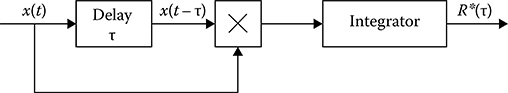
FIGURE 15.1 Correlator.

However, in practice, it is not convenient to restore the correlation function employing the sampling theorem. As a rule, there is a need to use an interpolation or smoothing of obtained discrete values. As it was proved empirically [1], it is worthwhile to define the discrete step in the following form:

$Δ τ \approx \frac{1}{5 - 10 f_{\max}} . (15.4)$

In doing so, 5 – 10 discrete estimates of correlation function correspond to each period of the highest frequency f_max of stochastic process spectral density.

Approximation to select the value Δτ based on the given error of straight-line interpolation of the correlation function estimate was obtained in Ref. [2]:

$Δ τ \approx \frac{1}{\hat{f}} \sqrt{0.2 | Δ ℛ |}, (15.5)$

where |Δℛ| is the maximum allowable value of interpolation error of the normalized correlation function ℛ(τ);

$\hat{f} = \sqrt{\frac{\int_{0}^{\infty} f^{2} S (f) d f}{\int_{0}^{\infty} S (f) d f}} (15.6)$

is the mean-square frequency value of the spectral density S(f) of the stochastic process ξ(t).

Sequential measurement of the correlation function at various values of τ = kΔτ, k = 0,1,2,…, v is not acceptable forever owing to long-time analysis, in the course of which the measurement conditions can change. For this reason, the correlators operating in parallel can be employed. The flowchart of multichannel correlator is shown in Figure 15.2. The voltage proportional to the discrete value of the estimated correlation function is observed at the output of each channel of the multichannel correlator. This voltage is supplied to the channel commutator, and the correlation function estimate, as a discrete time function, is formed at the commutator output. For this purpose, the commutator output is connected with the low-pass filter input and the low-pass filter possesses the filter time constant adjusted with request speed and a priori behavior of the investigated correlation function.

In principle, a continuous variation of delay is possible too, for example, the linear variation. In this case, the additional errors of correlation function measurements will arise. These errors are caused by variations in delay during averaging procedure. The acceptable values of delay variation velocity are investigated in detail based on the given additional measurement error.

Methods of the correlation function estimate can be classified into three groups based on the principle of realization of delay and other elements of correlators: analog, digital, and analog-to-digital. In turn, the analog measurement procedures can be divided on the methods employing a representation of investigated stochastic process both as the continuous process and as the sampled process. As a rule, physical delays are used by analog methods with continuous representation of investigated stochastic process. Under discretization of investigated stochastic process in time, the physical delay line can be changed by corresponding circuits. While using digital procedures to measure the correlation function estimate, the stochastic process is sampled in time and transformed into binary number by analog-to-digital conversion. Further operations associated with the signal delay, multiplication, and integration are carried out by the shift registers, summator, and so on.

Images

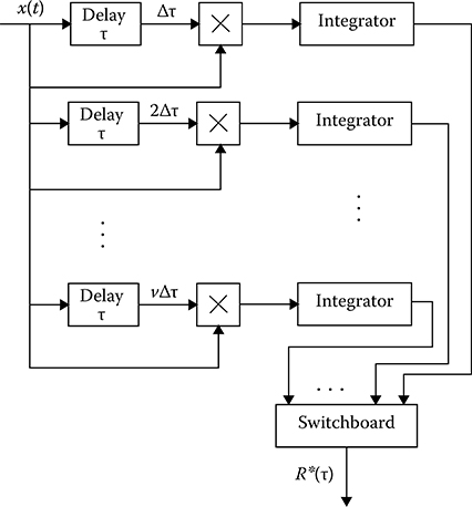
FIGURE 15.2 Multichannel correlator.

Define the statistical characteristics of the correlation function estimate (the bias and variance) given by (15.2). Averaging the correlation function estimate by an ensemble of realizations we obtain the unbiased correlation function estimate. The variance of correlation function estimate can be presented in the following form:

$Var {R^{*} (τ)} = \frac{1}{T^{2}} {\int^{}}_{0}^{T} {\int^{}}_{0}^{T} 〈 x (t_{1}) x (t_{1} - τ) x (t_{2}) x (t_{2} - τ) 〉 d t_{1} d t_{2} - R^{2} (τ) . (15.7)$

The fourth moment 〈x(t₁)x(t₁ − τ)x(t₂)x(t₂ − τ)〉 of Gaussian stochastic process can be determined as

$〈 x (t_{1}) x (t_{1} - τ) x (t_{2}) x (t_{2} - τ) 〉 = R^{2} (τ) + R^{2} (t_{2} - t_{1}) + R (t_{2} - t_{1} - τ) R (t_{2} - t_{1} + τ) . (15.8)$

Substituting (15.8) in (15.7) and transforming the double integral into a single one by introduction of the new variable t₂ − t₁ = τ, we obtain

$Var {R^{*} (τ)} = \frac{2}{T} {\int^{}}_{0}^{T} (1 - \frac{z}{T}) [R^{2} (z) + R (z - τ) (z + τ)] d z . (15.9)$

If the observation time interval [0, T] is much more in comparison with the correlation interval of the investigated stochastic process, (15.9) can be simplified as

$Var {R^{*} (τ)} = \frac{2}{T} {\int^{}}_{0}^{T} [R^{2} (z) + R (z - τ) R (z + τ)] d z . (15.10)$

Thus, we can see that maximum value of variance of the correlation function estimate corresponds to the case τ = 0 and is equal to the variance of stochastic process variance estimate given by (13.61) and (13.62). Minimum value of variance of the correlation function estimate corresponds to the case when τ ≫ τ_cor and is equal to one half of the variance of the stochastic process variance estimate.

In principle, we can obtain the correlation function estimate, the variance of which tends to approach to zero as τ → T. In this case, the estimate

$\tilde{R} (τ) = \frac{1}{T} {\int^{}}_{0}^{T - | τ |} x (t) x (t - τ) d t (15.11)$

can be considered as the correlation function estimate when the mathematical expectation of stochastic process is equal to zero. This correlation function estimate is characterized by the bias

$b [\tilde{R} (τ)] = \frac{| τ |}{T} R (τ) (15.12)$

and variance

$Var {\tilde{R} (τ)} = \frac{2}{T} {\int^{}}_{0}^{T - | τ |} (1 - \frac{z + | τ |}{T}) [R^{2} (z) + R (z - τ) R (z + τ)] d z . (15.13)$

In practice, a realization of the estimate given by (15.11) is more difficult to achieve compared to a realization of the estimate given by (15.2) since we need to change the value of the integration limits or observation time interval simultaneously with changing in the delay τ employing the one-channel measurer or correlator. Under real conditions of correlation function measurement, the observation time interval is much longer compared to the correlation interval of stochastic process. Because of this, the formula (15.13) can be approximated by the formula (15.10). Note that the correlation function measurement process is characterized by dispersion of estimate. If the correlation function estimate is given by (15.11), in the limiting case, the dispersion of estimate is equal to the square of estimate bias. For example, in the case of exponential correlation function given by (12.13) and under the condition T ≫ τ_cor, based on (15.10) we obtain

$Var {R^{*} (τ)} = \frac{σ^{4}}{α T} [1 + (2 α τ + 1) \exp {- 2 α τ}] . (15.14)$

As applied to the estimate given by (15.11) and the exponential correlation function, the variance of correlation function estimate can be presented in the following form [3]:

$Var {\tilde{R} (τ)} = \frac{σ^{4}}{α T} [1 + (2 α τ + 1) \exp {- 2 α τ}] - \frac{σ^{4}}{2 α^{2} T^{2}} [2 α τ + 1 (4 α τ + 6 α^{2} T^{2}) \exp {- 2 α τ}], (15.15)$

when the conditions T ≫ τ_cor and τ ≫ T are satisfied. Comparing (15.15) and (15.14), we can see that the variance of correlation function estimate given by (15.11) is lesser than the variance of correlation function estimate given by (15.2). When αT ≫ 1, we can discard this difference because it is defined as (αT)⁻¹.

In addition to the ideal integrator, any linear system can be used as an integrator to obtain the correlation function estimate analogously as under the definition of estimates of the variance and the mathematical expectation of the stochastic process. In this case, the function

$R^{*} (τ) = c {\int^{}}_{0}^{\infty} h (z) x (t - z) x (t - τ - z) d z (15.16)$

can be considered as the correlation function estimate, where, as before, the constant c is chosen from the condition of estimate unbiasedness

$c {\int^{}}_{0}^{\infty} h (z) d z = 1. (15.17)$

As applied to the Gaussian stochastic process, the variance of correlation function estimate as t → ∞ can be presented in the following form:

$Var {R^{*} (τ)} = c^{2} {\int^{}}_{0}^{T} {\int^{}}_{0}^{T} h (z_{1}) h (z_{2}) [R^{2} (z_{2} - z_{1}) + R (z_{2} - z_{1} - τ) R (z_{2} - z_{1} + τ)] d z_{1} d z_{2} . (15.18)$

Introducing new variables z₂ − z₁ = z, z₁ = υ we obtain

$\begin{array}{l} Var {R^{*} (τ)} = & c^{2} {\int^{}}_{0}^{T} [R^{2} (z) + R (z - τ) R (z + τ)] d z {\int^{}}_{0}^{T - τ} h (z + υ) h (υ) d υ \\ + {\int^{}}_{- T}^{0} [R^{2} (z) + R (z - τ) R (z + τ)] d z {\int^{}}_{0}^{T} h (z + υ) h (υ) d υ . \end{array} (15.19)$

Introducing the variables y = −z, υ − y and as T → ∞, we obtain

$Var {R^{*} (τ)} = c^{2} {\int^{}}_{0}^{\infty} [R^{2} (z) + R (z - τ) R (z + τ)] r_{h} (z) d z, (15.20)$

where the function r_h(z) is given by (12.131) as T − τ → ∞.

Now, consider how a sampling in time of stochastic process acts on the characteristics of correlation function estimate assuming that the investigated stochastic process is a stationary process. If a stochastic process with zero mathematical expectation is observed and investigated at discrete instants, the correlation function estimate can be presented in the following form:

$R^{*} (τ) = \frac{1}{N} {\sum^{}}_{i = 1}^{N} x (t_{i}) x (t_{i} - τ), (15.21)$

where N is the sample size. The correlation function estimate is unbiased, and the variance of correlation function estimate takes the following form:

$Var {R^{*} (τ)} = \frac{1}{N^{2}} {\sum^{}}_{i = 1}^{N} {\sum^{}}_{j = 1}^{N} 〈 x (t_{i}) x (t_{i} - τ) x (t_{j}) x (t_{j} - τ) 〉 - R^{2} (τ) . (15.22)$

As applied to the Gaussian stochastic process, the general formula, by analogy with the formula for the variance of correlation function estimate under continuous observation and analysis of stochastic process realization, is simplified and takes the following form:

$Var {R^{*} (τ)} = \frac{2}{N} {\sum^{}}_{i = 1}^{N} (1 - \frac{i}{N}) [R^{2} (i T_{p}) + R (i T_{p} - τ) (i T_{p} + τ)], (15.23)$

where we assume that the samples are taken over equal time intervals, that is, T = t_i − t_i−1.

If samples are pairwise independent, a definition of the variance of correlation function estimate given by (15.22) can be simplified; that is, we can use the following representation:

$Var {R^{*} (τ)} = \frac{1}{N^{2}} {\sum^{}}_{i = 1}^{N} 〈 x^{2} (t_{i}) x^{2} (t_{i} - τ) 〉 - \frac{1}{N} R^{2} (τ) . (15.24)$

As applied to the Gaussian stochastic process with pairwise independent samples, we can write

$Var {R^{*} (τ)} = \frac{σ^{4}}{N} [1 + ℛ^{2} (τ)], (15.25)$

where ℛ(τ) is the normalized correlation function of the observed stochastic process. As we can see from (15.25), the variance of correlation function estimate increases with an increase in the absolute magnitude of the normalized correlation function.

The obtained results can be generalized for the estimate of mutual correlation function of two mutually stationary stochastic processes, the realizations of which are x(t) and y(t), respectively:

$R_{x y}^{*} (τ) = \frac{1}{T} {\int^{}}_{0}^{T} x (t) y (t - τ) d t . (15.26)$

At this time, we assume that the investigated stochastic processes are characterized by zero mathematical expectations. Flowcharts to measure the mutual correlation function of stochastic processes are different from the flowcharts to measure the correlation functions presented in Figures 15.1 and 15.2 by the following: The processes x(t) and y(t − τ) or x(t − τ) and y(t) come in at the input of the mixer instead of the processes x(t) and x(t − τ). The mathematical expectation of mutual correlation function estimate can be presented in the following form:

$〈 R_{x y}^{*} (τ) 〉 = \frac{1}{T} {\int^{}}_{0}^{T} 〈 x (t) y (t - τ) 〉 d t = R_{x y} (τ) (15.27)$

that means the mutual correlation function estimate is unbiased.

As applied to the Gaussian stochastic process, the variance of mutual correlation function estimate takes the following form:

$Var {R_{x y}^{*} (τ)} = \frac{1}{T^{2}} {\int^{}}_{0}^{T} {\int^{}}_{0}^{T} {R_{x x} (t_{2} - t_{1}) R_{y y} (t_{2} - t_{1}) + R_{x y} [τ - (t_{2} - t_{1})] R_{x y} [τ + (t_{2} - t_{1})]} d t_{1} d t_{2} . (15.28)$

As before, we introduce the variables t₂ − t₁ = z and t₁ = υ and reduce the double integral to a single one. Thus, we obtain

${R_{x y}^{*} (τ)} = \frac{2}{T} {\int^{}}_{T}^{T} (1 - \frac{z}{T}) [R_{x r} (z) R_{y y} (z) + R_{x y} (τ - z) R_{x y} (τ + z)] d z . (15.29)$

At T ≫ τ_{cor_x}, T ≫ τ_{cor_y}, T ≫ x_{cor_xy}, where x_{cor_xy} is the interval of mutual correlation of stochastic processes and is determined analogously to (12.21), the integration limits can be expanded until [0, ∞) and we can neglect z/T in comparison with unit. Since the mutual correlation function can reach the maximum value at τ ≠ 0, the maximum variance of mutual correlation function estimate can be obtained at τ ≠ 0.

Now, consider the mutual correlation function between stochastic processes both at the input of linear system with the impulse response h(t) and at the output of this linear system. We assume the input process is the “white”. Gaussian stochastic process with zero mathematical expectation and the correlation function

$R_{x x} (τ) = \frac{N_{0}}{2} δ (τ) . (15.30)$

Denote the realization of stochastic process at the linear system input as x(t). Then, a realization of stochastic process at the linear system output in stationary mode can be presented in the following form:

$y (t) = {\int^{}}_{0}^{\infty} h (υ) x (t - υ) d υ = {\int^{}}_{0}^{\infty} h (t - υ) x (υ)) d υ . (15.31)$

The mutual correlation function between x(t − τ) and y(t) has the following form:

$R_{y x} (τ) = 〈 y (t) x (t - τ) 〉 = {\int^{}}_{0}^{\infty} h (υ) R_{x r} (υ - τ) d υ = {\begin{array}{l} 0.5 N_{0} h (τ), & τ \geq 0, \\ 0, & τ < 0. \end{array} (15.32)$

In (15.32) we assume that the integration process covers the point υ = 0.

As we can see from (15.32), the mutual correlation function of the stochastic process at the output of linear system in stationary mode, when the “white”. Gaussian noise excites the input of linear system, coincides with the impulse characteristic of linear system accurate with the constant factor. Thus, the method to measure the impulse response is based on the following relationship:

$h^{*} (τ) = \frac{2}{N_{0}} R_{y x}^{*} (τ) = \frac{2}{N_{0}} \frac{1}{T} {\int^{}}_{0}^{T} y (t) x (t - τ) d t, (15.33)$

Images

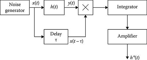
FIGURE 15.3 Measurement of linear system impulse response.

where y(t) is given by (15.31). The measuring process of the impulse characteristic of linear system is shown in Figure 15.3. Operation principles are clear from Figure 15.3.

Mathematical expectation of the impulse characteristic estimate

$〈 h^{*} (τ) 〉 = \frac{2}{N_{0} T} {\int^{}}_{0}^{T} {\int^{}}_{0}^{\infty} h (υ) 〈 x (t - υ) x (t - τ) 〉 d υ d t = h (τ), (15.34)$

that is, the impulse response estimate is unbiased. The variance of impulse characteristic estimate takes the following form:

$Var {h^{*} (τ)} = \frac{4}{N_{0}^{2} T^{2}} {\int^{}}_{0}^{T} {\int^{}}_{0}^{T} 〈 y (t_{1}) y (t_{2}) x (t_{1} - τ) x (t_{2} - τ) 〉 d t_{1} d t_{2} - h^{2} (τ) . (15.35)$

Since the stochastic process at the linear system input is Gaussian, the stochastic process at the output of the linear system is Gaussian, too. If the condition T ≫ τ_{cor_y} is satisfied, where τ_{cor_y} is the correlation interval of the stochastic process at the output of linear system, then the stochastic process at the output of linear system is stationary. For this reason, we can use the following representation for the variance of impulse characteristic estimate

$Var {h^{*} (τ)} = \frac{4}{N_{0}^{2} T^{2}} {\int^{}}_{0}^{T} {\int^{}}_{0}^{T} [R_{x x} (t_{2} - t_{1}) R_{y y} (t_{2} - t_{1}) + R_{y x} (t_{2} - t_{1} - τ) R_{y x} (t_{2} - t_{1} + τ)] d t_{1} d t_{2} . (15.36)$

Introducing new variables t₂ − t₁ = z, as before, the variance of impulse characteristic estimate can be presented in the following form:

$\begin{array}{l} Var {h^{*} (τ)} = & \frac{8}{N_{0}^{2} T} {\int^{}}_{0}^{T} (1 - \frac{z}{T}) [R_{x x} (z) R_{y y} (z) + R_{y x} (τ - z) R_{y x} (τ + z)] d t_{1} d t_{2} \\ + \frac{2}{T} {\int^{}}_{0}^{T} (1 - \frac{z}{T}) h (τ - z) h (τ + z) d z, \end{array} (15.37)$

where [3]

$R_{y y} (z) = \frac{N_{0}}{2} {\int^{}}_{0}^{\infty} h (υ) h (υ + | z |) d υ (15.38)$

is the correlation function of the stochastic process at the linear system output in stationary mode. While calculating the second integral in (15.37), we assume that the observation time interval [0, T] is much more compared to the correlation interval of the stochastic process at the output of linear system τ_{cor_y}. For this reason, in principle, we can neglect the term zT⁻¹ compared to the unit. In this case, the upper integration limits can be approximated by ∞. However, taking into consideration the fact that at τ < 0 the impulse response of linear system is zero, that is, h(τ) = 0, the integration limits with respect to the variable z must satisfy the following conditions:

${\begin{array}{l} 0 < z < \infty, \\ τ - z > 0, \\ τ + z > 0. \end{array} (15.39)$

Based on (15.39), we can find that 0 < z < τ. As a result, we obtain

$Var {h^{*} (τ)} = \frac{2}{T} {{\int^{}}_{0}^{\infty} h^{2} (υ) d υ + {\int^{}}_{0}^{τ} h (τ - υ) h (τ + υ) d υ} . (15.40)$

As applied to the impulse responses of the form

$\begin{matrix} h_{1} (τ) = \frac{1}{T_{1}}, & 0 < τ < T_{1}, & T > T_{1} \end{matrix} (15.41)$

and

$h_{2} (τ) = α \exp (- α τ), (15.42)$

the variances of impulse characteristic estimates can be presented in the following form:

$Var {h_{1}^{*} (τ)} = \frac{2}{T T_{1}} \times {\begin{array}{l} 1 + \frac{τ}{T_{1}}, & 0 \leq τ \leq 0.5 T_{1}, \\ 2 - \frac{τ}{T_{1}}, & 0.5 T_{1} \leq τ \leq T_{1}, \end{array} (15.43)$

$Var {h_{2}^{*} (τ)} = \frac{α}{T} [1 + 2 α τ \times \exp {- 2 α τ}] . (15.44)$

15.2 Correlation Function Estimation Based on its Expansion in Series

The correlation function of stationary stochastic process can be presented in the form of expansion in series with respect to earlier-given normalized orthogonal functions φ(t):

$R (τ) = {\sum^{}}_{k = 0}^{\infty} α_{k} φ_{k} (τ), (15.45)$

where the unknown coefficients α_k are given by

$α_{k} = \int_{- \infty}^{\infty} φ_{k} (τ) R (τ) d τ, (15.46)$

and (14.123) is true in the case of normalized orthogonal functions. The number of terms of the expansion in series (15.45) is limited by some magnitude v. Under approximation of correlation function by the expansion in series with the finite number of terms, the following error

$ε (τ) = R (τ) - {\sum^{}}_{k = 0}^{v} α_{k} φ_{k} (τ) = R (τ) - R_{v} (τ) (15.47)$

exists forever. This error can be reduced to an earlier-given negligible value by the corresponding selection of the orthogonal functions φ(t) and the number of terms of expansion in series.

Thus, the approximation accuracy will be characterized by the total square of approximated correlation function R_v(τ) deviation from the true correlation function R(i) for all possible values of the argument τ

$ε^{2} = \int_{- \infty}^{\infty} ε^{2} (τ) d τ \int_{- \infty}^{\infty} R^{2} (τ) d τ - {\sum^{}}_{k = 0}^{v} α_{k}^{2} . (15.48)$

Formula (15.48) is based on (15.45). The original method to measure the correlation function based on its representation in the form of expansion in series

$R_{v}^{*} (τ) = {\sum^{}}_{k = 0}^{v} α_{k}^{*} φ_{k} (τ) (15.49)$

by the earlier-given orthogonal functions φ_k(t) and measuring the weight coefficients α_k was discussed in Ref. [4]. According to (15.46), the following representation

$α_{k} = \lim_{T \to \infty} \int_{- \infty}^{\infty} φ_{k} (τ) {\frac{1}{T} {\int^{}}_{0}^{T} x (t) x (t - τ) d t} d τ (15.50)$

is true in the case of ergodic stochastic process with zero mathematical expectation. In line with this fact, the estimates of unknown coefficients of expansion in series can be obtained based on the following representation:

$α_{k}^{*} = \frac{1}{T} {\int^{}}_{0}^{T} x (t) {{\int^{}}_{0}^{\infty} x (t - τ) φ_{k} (τ) d τ} d t . (15.51)$

The integral in the braces

$y_{k} (t) = {\int^{}}_{0}^{\infty} x (t - τ) φ_{k} (τ) d τ (15.52)$

is the signal at the output of linear filter operating in stationary mode with impulse response given by

$h_{k} (t) = π {\begin{array}{l} 0 & if & t < 0, \\ φ_{k} (t) & if & t \geq 0, \end{array} (15.53)$

matched with the earlier-given orthogonal function φ(t). As we can see from (15.51), the mathematical expectation of estimate

$〈 α_{k}^{*} 〉 = {\int^{}}_{0}^{\infty} φ_{k} (τ) {\frac{1}{T} {\int^{}}_{0}^{T} 〈 x (t) x (t - τ) 〉 d t} d τ = {\int^{}}_{0}^{\infty} φ_{k} (τ) R (τ) d τ = α_{k} (15.54)$

is matched with the true value; in other words, the estimate of coefficients of expansion in series is unbiased.

The estimate variance of expansion in series coefficients can be presented in the following form:

$Var {α_{k}^{*}} = \frac{1}{T^{2}} {\int^{}}^{}_{0}^{T} {\int^{}}^{}_{0}^{T} 〈 x (t_{1}) x (t_{2}) y_{k} (t_{1}) y_{k} (t_{2}) 〉 d t_{1} d t_{2} - {\frac{1}{T} {\int^{}}^{}_{0}^{T} 〈 x (t) y_{k} (t) 〉 d t}^{2} . (15.55)$

As applied to the stationary Gaussian stochastic process, the stochastic process forming at the output of orthogonal filter will also be the stationary Gaussian stochastic process for the considered case. Because of this, we can write

$Var {α_{k}^{*}} = \frac{1}{T^{2}} {\int^{}}_{0}^{T} {\int^{}}_{0}^{T} [R (t_{2} - t_{1}) R_{y k} (t_{2} - t_{1}) + R_{x y_{k}} (t_{2} - t_{1}) R_{y_{k} x} (t_{2} - t_{1})] d t_{1} d t_{2}, (15.56)$

where

$R_{y_{k}} (τ) = {\int^{}}_{0}^{\infty} {\int^{}}_{0}^{\infty} R (τ + v - κ) φ_{k} (κ) φ_{k} (v) d κ d v; (15.57)$

$R_{x y_{k}} (τ) = {\int^{}}_{0}^{\infty} R (τ - v) φ_{k} (v) d v; (15.58)$

$R_{y_{k} x} (τ) = {\int^{}}_{0}^{\infty} R (τ + v) φ_{k} (v) d v . (15.59)$

Introducing new variables t₂ − t₁ = τ, t₁ = t and changing the order of integration analogously as shown in Section 12.4, we obtain

$Var {α_{k}^{*}} = \frac{2}{T} {\int^{}}_{0}^{T} (1 - \frac{τ}{T}) {\int^{}}_{0}^{T} {\int^{}}_{0}^{T} [R (τ) R_{y_{k}} (τ) + R_{x y_{k}} (τ) R_{y_{k} x} (τ)] d τ . (15.60)$

Images

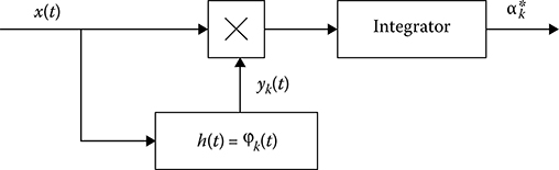
FIGURE 15.4 One-channel measurer of coefficients α_k.

Taking into consideration that

$〈 {(α_{k}^{*})}^{2} 〉 = Var {α_{k}^{*}} + α_{k}^{2} (15.61)$

and the condition given by (14.123), we can define the “integral” variance of correlation function estimate

$Var {R_{v}^{*} (τ)} = \int_{- \infty}^{\infty} 〈 {[R_{v}^{*} (τ) - 〈 R_{v}^{*} (τ) 〉]}^{2} 〉 d τ = \sum_{k = 0}^{v} Var {α_{k}^{*}} . (15.62)$

As we can see from (15.62), the variance of correlation function estimate increases with an increase in the number of terms of expansion in series v. Because of this, we must take into consideration choosing the number of terms under expansion in series.

The foregoing formulae allow us to present the flowchart of correlation function measurer based on the expansion of this correlation function in series and the estimate of coefficients of this expansion in series Figure 15.4 represents the one-channel measurer of the current value of the coefficient $α_{k}^{*}$ . Operation of measurer is clear from Figure 15.4. One of the main elements of block diagram of the correlation function measurer is the generator of orthogonal signals or functions (the orthogonal filters with the impulse response given by [15.53]). If the pulse with short duration τ_p that is much shorter than the filter constant time and amplitude $τ_{p}^{- 1}$ excites the input of the orthogonal filter, then a set of orthogonal functions φ_k(t) are observed at the output of orthogonal filters.

The flowchart of correlation function measurer is shown in Figure 15.5. Operation control of the correlation function measurer is carried out by the synchronizer that stimulates action on the generator of orthogonal signals and allows us to obtain the correlation function estimate with period that is much longer compared to the orthogonal signal duration.

The functions using the orthogonal Laguerre polynomials given by (14.72) and presented in the following form

$L_{k} (α t) = \exp {α t} \frac{d^{k} [t^{k} \exp {- α t}]}{d t^{k}} = {\sum^{}}_{μ = 0}^{k} \frac{{(- α t)}^{μ} {(k!)}^{2}}{(k - μ)! {(μ!)}^{2}} (15.63)$

are the simplest among a set of orthogonal functions, where α characterizes a polynomial scale in time. To satisfy (14.123), in this case, the orthogonal functions φ_k(t) take the following form:

$φ_{k} (t) = \frac{1}{k!} \sqrt{α} \exp {- 0.5 α t} L_{k} (α t) . (15.64)$

Images

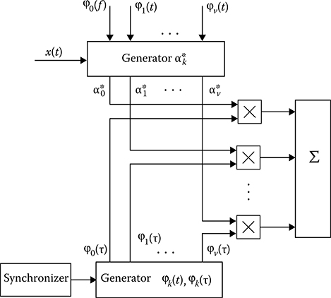
FIGURE 15.5 Measurer of correlation function.

Carrying out the Laplace transform

$φ_{k} (p) = {\int^{}}_{0}^{\infty} \exp {- p t} φ_{k} (t) d t, (15.65)$

we can find that the considered orthogonal functions correspond to the transfer functions

$φ_{k} (p) = \frac{2}{\sqrt{α}} \times \frac{0.5 α}{p + 0.5 α} {[\frac{p - 0.5 α}{p + 0.5 α}]}^{k} . (15.66)$

The multistep filter based on RC elements, that is, α = 2(RC)⁻¹, which has the transfer characteristic given by (15.66) accurate with the constant factor 2α^−0.5 is shown in Figure 15.6. The phase inverter is assigned to generate two signals with equal amplitudes and shifted by phase on 90° and the amplifiers compensate attenuation in filters and ensure decoupling between them.

If the stationary stochastic process is differentiable ν times, the correlation function R(τ) of this process can be approximated by expansion in series about the point τ = 0:

$R (τ) \approx R_{v} (τ) = {\sum^{}}_{i = 0}^{v} {\frac{d^{2 i} R (τ)}{d τ^{2 i}} |}_{τ = 0} \times \frac{τ^{2 i}}{(2 i)!} . (15.67)$

The approximation error of the correlation function is defined as

$ε (τ) = R (τ) - R_{v} (τ) . (15.68)$

The even 2ith derivatives of the correlation function at the point τ = 0 accurate within the coefficient (−1)ⁱ are the variances of ith derivatives of the stochastic process

${(- 1)}^{i} {\frac{d^{2 i} R (τ)}{d τ^{2 i}} |}_{τ = 0} = 〈 {[\frac{d^{i} ξ (t)}{d t^{i}}]}^{2} 〉 = {Var}_{_{i}} . (15.69)$

Images

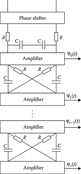
FIGURE 15.6 Multistep RC filter.

As applied to the ergodic stochastic process, the coefficients of expansion in series given by (15.67) can be presented in the following form:

$α_{i} = {\frac{d^{2 i} R (τ)}{d τ^{2 i}} |}_{τ = 0} = {(- 1)}^{i} \lim_{T \to \infty} \frac{1}{T} {\int^{}}_{0}^{T} {\frac{d^{i} x (t)}{d t^{i}}}^{2} d t . (15.70)$

In the case when the observation time interval is finite, the estimate $α_{i}^{*}$ of the coefficient α_i is defined as

$α_{i}^{*} = {(- 1)}^{i} \frac{1}{T} {\int^{}}_{0}^{T} {\frac{d^{i} x (t)}{d t^{i}}}^{2} d t . (15.71)$

The correlation function estimate takes the following form:

$R^{*} (τ) = {\sum^{}}_{i = 1}^{v} \frac{α_{i}^{*} τ^{2 i}}{(2 i)!} . (15.72)$

Flowchart of measurer based on definition of the coefficients of correlation function expansion in power series is shown in Figure 15.7. The investigated realization x(t) is differentiable ν times. The obtained processes y_i(t) = dⁱx(t)/dtⁱ are squared and integrated within the limits of the observation time interval [0, T] and come in at the input of calculator with corresponding signs. According to (15.72), the correlation function estimate is formed at the calculator output. Define the statistical characteristics of the coefficient estimate $α_{i}^{*}$ . The mathematical expectation of the estimate $α_{i}^{*}$ has the following form:

Images

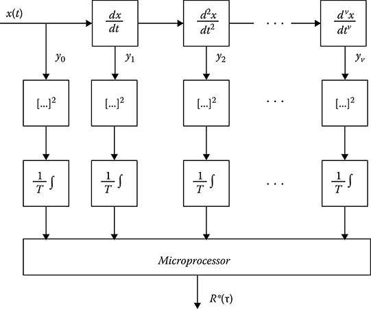
FIGURE 15.7 Correlation function measurement.

$〈 α_{i}^{*} 〉 = {(- 1)}^{i} \frac{1}{T} {\int^{}}_{0}^{T} 〈 {\frac{d^{i} x (t)}{d t^{i}}}^{2} 〉 d t . (15.73)$

We can see that

${\frac{d^{i} x (t)}{d t^{i}}}^{2} = {\frac{\partial^{2 i} R (t_{1} - t_{2})}{\partial r_{1}^{i} \partial r_{2}^{i}} |}_{t_{1} = t_{2} = t} = {(- 1)}^{i} {\frac{d^{2 i} R (τ)}{d τ^{2 i}} |}_{τ = 0} . (15.74)$

An introduction of new variables t₂ − t₁ = τ, t₂ = t is made. Substituting (15.74) into (15.73), we see that the estimates of coefficients of expansion in series are unbiased. The correlation function of estimates is

$R_{i p} = 〈 α_{i}^{*} α_{p}^{*} 〉 - 〈 α_{i}^{*} 〉 〈 α_{p}^{*} 〉, (15.75)$

where

$〈 α_{i}^{*} α_{p}^{*} 〉 = {(- 1)}^{(i + p)} \frac{1}{T^{2}} {\int^{}}_{0}^{T} {\int^{}}_{0}^{T} 〈 {\frac{d^{i} x (t_{1})}{d t_{1}^{i}}}^{2} {\frac{d^{p} x (t_{1})}{d t_{2}^{p}}}^{2} 〉 d t_{1} d t_{2} . (15.76)$

As applied to the Gaussian stochastic process, its derivative is Gaussian too. Because of this, we can write

$\begin{array}{l} \begin{array}{l} 〈 {\frac{d^{i} x (t_{1})}{d t_{1}^{i}}}^{2} {\frac{d^{p} x (t_{1})}{d t_{2}^{p}}}^{2} 〉 & = 〈 {\frac{d^{i} x (t_{1})}{d t_{1}^{i}}}^{2} 〉 〈 {\frac{d^{p} x (t_{1})}{d t_{2}^{p}}}^{2} 〉 + 2 {\frac{\partial^{(i + p)} 〈 x (t_{1}) x (t_{2}) 〉}{\partial r_{1}^{i} \partial r_{2}^{p}}}^{2} \\ = {Var}_{i} \times {Var}_{p} + 2 {\frac{\partial^{(i + p)} R (t_{2} - t_{1})}{\partial r_{1}^{i} \partial r_{2}^{p}}}^{2} . \end{array} \end{array} (15.77)$

Substituting (15.77) into (15.76) and then into (15.75), we obtain

$R_{i p} = {(- 1)}^{(i + p)} \frac{2}{T^{2}} {\int^{}}_{0}^{T} {\int^{}}_{0}^{T} {\frac{\partial^{(i + p)} R (t_{2} - t_{1})}{\partial r_{1}^{i} \partial r_{2}^{p}}}^{2} d t_{1} d t_{2} . (15.78)$

Introducing new variables t₂ − t₁ = τ, t₂ = t and changing the order of integration, we obtain

$R_{i p} = \frac{4}{T} {\int^{}}_{0}^{T} (1 - \frac{τ}{T}) {\frac{d^{(i + p)} R (τ)}{d τ^{(i + p)}}}^{2} d τ . (15.79)$

If the observation time interval is much longer than the correlation interval of stochastic process and its derivatives, we can write

$R_{i p} = \frac{2}{T} \int_{- \infty}^{\infty} {\frac{d^{(i + p)} R (τ)}{d τ^{(i + p)}}}^{2} d τ . (15.80)$

As applied to the conditions, for which (15.80) is appropriate, the derivatives of the correlation function can be written using the spectral density S(ω) of the stochastic process:

$\frac{d^{(i + p)} R (τ)}{d τ^{(i + p)}} = \frac{1}{2 π} \int_{- \infty}^{\infty} {(j ω)}^{(i + p)} S (ω) \exp {j ω τ} d ω . (15.81)$

Then

$R_{i p} = \frac{1}{T π} \int_{- \infty}^{\infty} ω^{2 (i + p)} S^{2} (ω) d ω . (15.82)$

The variance of the estimate $α_{i}^{*}$ of expansion in series coefficients can be presented in the following form:

$Var {α_{i}^{*}} = \frac{1}{T π} \int_{- \infty}^{\infty} ω^{4 i} S^{2} (ω) d ω . (15.83)$

Let us define the deviation of correlation function estimate from the approximated value, namely,

$ε (τ) = R_{v} (τ) - R_{v}^{*} (τ) . (15.84)$

Averaging ɛ(τ) by realizations of the investigated stochastic process, we can see that in the considered case 〈ɛ(τ)〉 = 0, which means the bias of correlation function estimate does not increase due to the finite observation time interval.

The variance of correlation function estimate can be presented in the following form:

$Var {R_{v}^{*} (τ)} = {\sum^{}}_{i = 1}^{v} {\sum^{}}_{p = 1}^{v} \frac{τ^{2 (i + p)}}{(2 i)! (2 p)!} \frac{4}{T} {\int^{}}_{0}^{T} (1 - \frac{τ}{T}) {\frac{d^{(i + p)} R (τ)}{d τ^{(i + p)}}}^{2} d τ . (15.85)$

At T ≫ τ_cor, we can write

$Var {R_{v}^{*} (τ)} = \frac{1}{T π} {\sum^{}}_{i = 1}^{v} {\sum^{}}_{p = 1}^{v} \frac{τ^{2 (i + p)}}{(2 i)! (2 p)!} {\int^{}}_{- \infty}^{\infty} ω^{2 (i + p)} S^{2} (ω) d ω . (15.86)$

Let the correlation function of the stochastic process be approximated by

$R (τ) = σ^{2} \exp {- α^{2} τ^{2}}, (15.87)$

which corresponds to the spectral density defined as

$S (ω) = σ^{2} \frac{\sqrt{π}}{α} \exp {- \frac{ω^{2}}{4 α^{2}}} . (15.88)$

Substituting (15.88) into (15.86), we obtain

$Var {R_{v}^{*} (τ)} = \frac{σ^{4} \sqrt{2 π}}{T α} {\sum^{}}_{i = 1}^{v} {\sum^{}}_{p = 1}^{v} \frac{[2 (i + p) - 1]!!}{(2 i)! (2 p)!} {(α τ)}^{2 (i + p)}, (15.89)$

where

$[2 (i + p) - 1]! = 1 \times 3 \times 5 \times ... \times [2 (i + p) - 1] . (15.90)$

As we can see from (15.89), the variance of correlation function estimate increases with an increase in the number of terms under correlation function expansion in power series.

15.3 Optimal Estimation of Gaussian Stochastic Process Correlation Function Parameter

In some practical conditions, the correlation function of stochastic process can be measured accurately with some parameters defining a character of its behavior. In this case, a measurement of correlation function can be reduced to measurement or estimation of unknown parameters of correlation function. Because of this, we consider the optimal estimate of arbitrary correlation function parameter assuming that the investigated stochastic process. ξ(t) is the stationary. Gaussian stochastic process observed within the limits of time interval [0, T] in the background of Gaussian stationary noise ζ(t) with known correlation function.

Thus, the following realization

$\begin{matrix} y (t) = x (t, l_{0}) + n (t), & 0 \leq t \leq T \end{matrix} (15.91)$

comes in at the measurer input, where x(t, l₀) is the realization of the investigated Gaussian stochastic process with the correlation function R_x(t₁, t₂, l) depending on the estimated parameter l; n(t) is the realization of Gaussian noise with the correlation function R_n(t₁, t₂). True value of estimated parameter of the correlation function R_x(t₁, t₂, l) is l₀. Thus, we assume that the mathematical expectation of both the realization x(t, l₀) and the realization n(t) is equal to zero and the realizations. x(t, l₀) and n(t) are statistically independent of each other. Based on input realization, the optimal receiver should form the likelihood ratio functional Λ(l) or some monotone function of the likelihood ratio. The stochastic process η(t) with realization given by (15.91) is the Gaussian stochastic process with zero mathematical expectation and the correlation function

$R_{y} (t_{1}, t_{2}, l) = R_{x} (t_{1}, t_{2}, l) + R_{n} (t_{1}, t_{2}) . (15.92)$

As applied to the investigated stochastic process η(t), the likelihood functional can be presented in the following form [5]:

$Λ (l) = \exp {\frac{1}{2} {\int^{}}_{0}^{T} {\int^{}}_{0}^{T} y (t_{1}) y (t_{2}) [ϑ_{n} (t_{1}, t_{2}) - ϑ_{x} (t_{1}, t_{2}; l)] d t_{1} d t_{2} - \frac{1}{2} H (l)} . (15.93)$

We can write the derivative of the function H(l) in the following form:

$\frac{d H (l)}{d l} = {\int^{}}_{0}^{T} {\int^{}}_{0}^{T} \frac{\partial R_{x} (t_{1}, t_{2}, l)}{\partial l} ϑ_{x} (t_{1}, t_{2}; l) d t_{1} d t_{2} (15.94)$

and the functions ϑ_x(t₁, t₂; l) and ϑ_n(t₁, t₂) can be found from the following equations:

${\int^{}}_{0}^{T} [R_{x} (t_{1}, t_{2}, l) + R_{n} (t_{1}, t_{2})] ϑ_{x} (t_{1}, t_{2}; l) d t = δ (t_{2} - t_{1}), (15.95)$

${\int^{}}_{0}^{T} R_{n} (t_{1}, t_{2}) ϑ_{n} (t_{1}, t_{2}) d t = δ (t_{2} - t_{1}) . (15.96)$

Evidently, we can use the logarithmic term of the likelihood functional depending on the observed data as the signal at the receiver output

$M_{1} (l) = \frac{1}{2} {\int^{}}_{0}^{T} {\int^{}}_{0}^{T} y (t_{1}) y (t_{2}) ϑ (t_{1}, t_{2}; l) d t_{1} d t_{2}, (15.97)$

where

$ϑ (t_{1}, t_{2}; l) = ϑ_{n} (t_{1}, t_{2}) - ϑ_{x} (t_{1}, t_{2}; l) . (15.98)$

We suppose that the correlation intervals of the stochastic processes ξ(t) and ζ(t) are sufficiently small compared to the observation time interval [0, T]. In this case, we can use infinite limits of integration. Under this assumption, we have

${\begin{array}{l} ϑ_{x} (t_{1}, t_{2}; l) = ϑ_{x} (t_{1} - t_{2}; l), \\ ϑ_{n} (t_{1}, t_{2}) = ϑ_{n} (t_{1} - t_{2}), \end{array} (15.99)$

and

$ϑ (t_{1}, t_{2}; l) = ϑ (t_{1} - t_{2}; l) . (15.100)$

Introducing new variables t₂ − t₁ = τ, t₂ = t and changing the order of integration, we obtain

$M_{1} (l) = \frac{1}{2} {{\int^{}}_{0}^{T} ϑ (τ; l) {\int^{}}_{0}^{T - τ} y (t + τ) y (t) d t d τ + {\int^{}}_{- T}^{0} ϑ (τ; l) {\int^{}}_{0}^{T} y (t + τ) y (t) d t d τ} . (15.101)$

Introducing new variables τ = −τ′, t′ = t + τ = τ − τ′ and taking into consideration that the correlation interval of stochastic process η(t) is shorter compared to the observation time interval [0, T], we can write

$M_{1} (l) = T {\int^{}}_{0}^{T} R_{y}^{*} (τ) ϑ (τ; l) d τ, (15.102)$

where

$R_{y}^{*} (τ) = \frac{1}{T} {\int^{}}_{0}^{T - τ} y (t) y (t + τ) d t \approx \frac{1}{T} {\int^{}}_{0}^{T} y (t) y (t - τ) d t (15.103)$

is the correlation function estimate of investigated input process consisting of additive mixture of the signal and noise.

Applying the foregoing statements to (15.94), we obtain

$\frac{d H (l)}{d l} = 2 T {\int^{}}_{0}^{T} \frac{\partial R_{x} (τ; l)}{\partial l} ϑ_{x} (τ; l) d τ . (15.104)$

Substituting (15.102) and (15.104) into (15.93), we obtain

$Λ (l) = \exp {T {\int^{}}_{0}^{T} R_{y}^{*} (τ) ϑ (τ; l) d τ - \frac{1}{2} H (l)} . (15.105)$

In the case, when the observation time interval [0, T] is much longer compared to the correlation interval of the investigated stochastic process, we can use the spectral representation of the function given by (15.100)

$ϑ (τ; l) = \frac{1}{2 π} \int_{- \infty}^{\infty} [ϑ_{n} (ω) - ϑ_{x} (ω; l)] \exp {j ω τ} d ω . (15.106)$

Then (15.104) takes the following form:

$\frac{d H (l)}{d l} = \frac{T}{2 π} {\int^{}}_{0}^{T} \frac{\partial S_{x} (ω; l)}{\partial l} ϑ_{x} (ω; l) d ω . (15.107)$

In (15.106) and (15.107), ϑ_n(ω), ϑ_x(ω; l), and S_x(ω; l) are the Fourier transforms of the corresponding functions ϑ_n(τ), ϑ_x(τ; l), and R_x(τ; l). Applying the Fourier transform to (15.95) and (15.96), we obtain

${{\begin{array}{l} R_{n} (ω) ϑ_{n} (ω) = 1, \\ ϑ_{x} (ω; l) [S_{n} (ω) + R_{x} (ω; l)] = 1. \end{array} (15.108)$

Taking into consideration (15.107) and (15.108), we can write

$ϑ (τ; l) = \frac{1}{2 π} \int_{- \infty}^{\infty} \frac{S_{x} (ω; l) S_{n}^{- 1} (ω)}{S_{x} (ω; l) + S_{n} (ω)} \exp {j ω τ} d ω, (15.109)$

$H (l) = \frac{T}{2 π} \int_{- \infty}^{\infty} \ln [1 + \frac{S_{x} (ω; l)}{S_{n} (ω)}] d ω . (15.110)$

The signal at the optimal receiver output takes the following form:

$M (l) = T {\int^{}}_{0}^{T} R_{y}^{*} (τ) ϑ (τ; l) d τ - \frac{1}{2} H (l) . (15.111)$

Flowchart of the optimal measurer is shown in Figure 15.8. This measurer operates in the following way. The correlation function $R_{y}^{*} (τ)$ is defined based on the input realization of additive mixture of the signal and noise. This correlation function is integrated as the weight function with the signal ϑ(τ; l). The signals forming at the outputs of the integrator and generator of the function H(l) come

Images

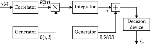
FIGURE 15.8 Optimal measurement of correlation function parameter.

in at the input of summator. Thus, the receiver output signal is formed. The decision device issues the value of the parameter l_m, under which the output signal takes the maximum value.

If the correlation function of the investigated Gaussian stochastic process has several unknown parameters l = {l₁, l₂, …, l}, then the likelihood ratio functional can be found by (15.93) changing the scalar parameter l. on the vector parameter l and the function H(l) is defined by its derivatives

$\frac{\partial H (l)}{\partial l_{i}} = {\int^{}}_{0}^{T} {\int^{}}_{0}^{T} \frac{\partial R_{x} (t_{1}, t_{2}; l)}{\partial l_{i}} ϑ_{x} (t_{1}, t_{2}; l) d t_{1} d t_{2} . (15.112)$

The function ϑ_x(t₁, t₂; l) is the solution of integral equation that is analogous to (15.95).

To obtain the estimate of maximum likelihood ratio of the correlation function parameter the optimal measurer (receiver) should define an absolute maximum l_m of logarithm of the likelihood ratio functional

$M (l) = \frac{1}{2} {\int^{}}_{0}^{T} {\int^{}}_{0}^{T} y (t_{1}) y (t_{2}) [ϑ_{n} (t_{1}, t_{2}) - ϑ_{x} (t_{1}, t_{2}, l)] d t_{1} d t_{2} - \frac{1}{2} H (l) . (15.113)$

To define the characteristics of estimate of the maximum likelihood ratio l_m introduce the signal

$s (l) = 〈 M (l) 〉 (15.114)$

and noise

$n (l) = M (l) - 〈 M (l) 〉 (15.115)$

functions. Then (15.113) takes the following form:

$M (l) = s (l) + n (l) . (15.116)$

Prove that if the noise component is absent in (15.116), that is, n(l) = 0, the logarithm of likelihood ratio functional reaches its maximum at l = l₀, that is, when the estimated parameter takes the true value. Define the first and second derivatives of the signal function given by (15.114) at the point l = l₀:

${\frac{d s (l)}{d l} |}_{l = l_{0}} = {〈 \frac{d M (l)}{d l} 〉 |}_{l = l_{0}} . (15.117)$

Substituting (15.113) into (15.117) and averaging by realizations y(t), we obtain

$\begin{array}{l} \begin{array}{l} {\frac{d s (l)}{d l} |}_{l = l_{0}} & = {- \frac{1}{2} {\int^{}}_{0}^{T} {\int^{}}_{0}^{T} [R_{n} (t_{1}, t_{2}) + R_{x} (t_{1}, t_{2}; l)] \frac{\partial ϑ_{x} (r_{1}, r_{2}; l)}{\partial l} d t_{1} d t_{2} - \frac{1}{2} {\int^{}}_{0}^{T} {\int^{}}_{0}^{T} ϑ_{x} (t_{1}, t_{2}; l) \frac{\partial R_{x} (t_{1}, t_{2}; l)}{\partial l} d t_{1} d t_{2}}_{l = l_{0}} \\ = - \frac{1}{2} {\frac{d}{d t} {\int^{}}_{0}^{T} {\int^{}}_{0}^{T} [R_{n} (t_{1}, t_{2}) + R_{x} (t_{1}, t_{2}; l)] ϑ_{x} (t_{1}, t_{2}; l) d t_{1} d t_{2}}_{l = l_{0}} . \end{array} \end{array} (15.118)$

Since

$R (t_{1}, t_{2}; l) = R_{n} (t_{1}, t_{2}) + R_{x} (t_{1}, t_{2}; l) = R (t_{2}, t_{1}; l), (15.119)$

in accordance with (15.95) we have

${\frac{d s (l)}{d l} |}_{l = l_{0}} = - \frac{1}{2} {\int^{}}_{0}^{T} {\frac{d}{d l} {\int^{}}_{0}^{T} [R_{n} (t_{2}, t_{1}) + R_{x} (t_{2}, t_{1} : l)] ϑ_{x} (t_{1}, t_{2}; l) d t_{1}}_{l = l_{0}} d t_{2} = 0. (15.120)$

Now, let us define the second derivative of the signal component at the point l = l₀:

$\begin{array}{l} {\frac{d^{2} s (l)}{d l^{2}} |}_{_{l = l_{0}}} & = {〈 \frac{d^{2} M (l)}{d l^{2}} 〉 |}_{l = l_{0}} \\ = \frac{1}{2} {{\int^{}}_{0}^{T} {\int^{}}_{0}^{T} \frac{\partial R_{x} (t_{2}, t_{1} : l)}{\partial l} \frac{\partial ϑ_{x} (t_{1}, t_{2}; l)}{\partial l} d t_{1} d t_{2} - \frac{d^{2}}{d l^{2}} {\int^{}}_{0}^{T} {\int^{}}_{0}^{T} [R_{n} (t_{2}, t_{1}) + R_{x} (t_{2}, t_{1} : l)] ϑ_{x} (t_{1}, t_{2}; l) d t_{1} d t_{2}}_{l = l_{0}} \end{array} (15.121)$

In accordance with (15.95) we can write

$\begin{array}{l} {\frac{d^{2}}{d l^{2}} {\int^{}}_{0}^{T} {\int^{}}_{0}^{T} [R_{n} (t_{2}, t_{1}) + R_{x} (t_{2}, t_{1} : l)] ϑ_{x} (t_{1}, t_{2}; l) d t_{1} d t_{2}}_{l = l_{0}} \\ = {\int^{}}_{0}^{T} {\frac{d^{2}}{d l^{2}} {\int^{}}_{0}^{T} [R_{n} (t_{2}, t_{1}) + R_{x} (t_{2}, t_{1} : l)] ϑ_{x} (t_{1}, t_{2}; l) d t_{1}}_{l = l_{0}} d t_{2} = 0. \end{array} (15.122)$

Because of this

${\frac{d^{2} s (l)}{d l^{2}} |}_{l = l_{0}} = \frac{1}{2} {{\int^{}}_{0}^{T} {\int^{}}_{0}^{T} \frac{\partial R_{x} (t_{2}, t_{1} : l)}{\partial l} \frac{\partial ϑ_{x} (t_{1}, t_{2}; l)}{\partial l} d t_{1} d t_{2}}_{l = l_{0}} . (15.123)$

Let us prove that the condition

${\frac{d^{2} s (l)}{d l^{2}} |}_{l = l_{0}} < 0 (15.124)$

is satisfied forever. For this purpose, we define the averaged quadratic first derivative of the likelihood ratio functional logarithm at the point l = l₀

$m^{2} = 〈 {{\frac{d M (l)}{d l} |}_{l = l_{0}}}^{2} 〉 = 〈 {{\frac{d N (l)}{d l} |}_{l = l_{0}}}^{2} 〉, (15.125)$

which is a positive value. Substituting (15.91) into (15.113), differentiating by l, and averaging by realizations y(t), we obtain the second central moment of the first derivative of the likelihood ratio functional logarithm:

$\begin{array}{l} \frac{\partial^{2}}{\partial l_{1} \partial l_{2}} 〈 [M (l_{1}) - 〈 M (l_{1}) 〉] [M (l_{2}) - 〈 M (l_{2}) 〉] 〉 \\ = \frac{1}{2} {\int^{}}_{0}^{T} {\int^{}}_{0}^{T} {\int^{}}_{0}^{T} {\int^{}}_{0}^{T} [R_{n} (t_{1}, t_{3}) + R_{x} (t_{1}, t_{3}; l_{0})] [R_{n} (t_{2}, t_{4}) + R_{x} (t_{2}, t_{4}; l_{0})] \\ \times \frac{\partial ϑ_{x} (r_{1}, r_{2}; l_{1})}{\partial l_{1}} \frac{\partial ϑ_{x} (t_{3}, t_{4}; l_{2})}{\partial l_{2}} d t_{1} d t_{2} d t_{3} d t_{4} . \end{array} (15.126)$

Assuming l₂ = l₁ = l₀ and taking into consideration that

${\int^{}}_{0}^{T} [R_{n} (t_{1}, t) + R_{x} (t_{1}, t; l_{0})] \frac{\partial ϑ_{x} (t_{1}, t_{2}; l)}{\partial l_{1}} d t = - {\int^{}}_{0}^{T} ϑ_{x} (t, t_{2}; l) \frac{\partial R_{x} (t_{1}, t; l)}{\partial l} d t, (15.127)$

we obtain

$\begin{array}{l} \begin{array}{l} m^{2} & = - {\frac{1}{2} {\int^{}}_{0}^{T} {\int^{}}_{0}^{T} {\int^{}}_{0}^{T} {\int^{}}_{0}^{T} [R_{n} (t_{2}, t_{4}) + R_{x} (t_{2}, t_{4}; l_{0})] ϑ_{x} (t_{1}, t_{2}; l) \frac{\partial R_{x} (t_{1}, t_{3}; l)}{\partial l} \frac{\partial ϑ_{x} (t_{3}, t_{4}; l)}{\partial l} d t_{l} d t_{2} d t_{3} d t_{4}}_{l = l_{0}} \\ = - {\frac{1}{2} {\int^{}}_{0}^{T} {\int^{}}_{0}^{T} \frac{\partial R_{x} (t_{1}, t_{2}; l)}{\partial l} \frac{\partial ϑ_{x} (t_{1}, t_{2}; l)}{\partial l} d t_{1} d t_{2}}_{l = l_{0}} . \end{array} \end{array} (15.128)$

In (15.128) we have implemented (15.95) again. Comparing (15.128) with (15.123), we can see that

${\frac{d^{2} s (l)}{d l^{2}} |}_{l = l_{0}} = - m^{2} (15.129)$

and, consequently, (15.124) is satisfied forever

Introduce the signal-to-noise ratio (SNR)

$SNR = \frac{s^{2} (l_{0})}{〈 n^{2} (l_{0}) 〉} (15.130)$

and the normalized signal and noise functions

${\begin{array}{l} S (l) = \frac{s (l)}{s (l_{0})}, \\ N (l) = \frac{n (l)}{\sqrt{〈 n^{2} (l_{0}) 〉}} . \end{array} (15.131)$

Taking into consideration (15.120), (15.124), and (15.131), we can see that

${\begin{array}{l} \max S (l) = S (l_{0}) = 1, \\ 〈 N^{2} (l_{0}) 〉 = 1. \end{array} (15.132)$

In addition, as follows from the definition, the mathematical expectation of the noise function n(l) is zero. Taking into consideration the introduced notations, we can write the logarithm of the likelihood ratio functional in the following form:

$M (l) = s (l_{0}) [S (l) + ε N (l)], (15.133)$

where $ɛ = 1 / \sqrt{S N R}$ . Taking into consideration (15.133), the likelihood ratio equation for the estimate of correlation function parameter of Gaussian stochastic process can be presented in the following form:

${\frac{d S (l)}{d l} + ε \frac{d N (l)}{d l}}_{l = l_{m}} = 0. (15.134)$

Usually, under the measurement of stochastic process parameters, SNR is high and, consequently, ɛ ≪ 1. Then, by analogy with Ref. [5], the approximated solution of likelihood ratio equation can be searched in the form of expansion in power series

$l_{m} = l_{0} + ε l_{1} + ε^{2} l_{2} + ε^{3} l_{3} + .... (15.135)$

To define the approximations l₁, l₂, l₃ and grouping the terms with small value ɛ of the same power, we obtain

$s_{1} + ε (l_{1} s_{2} + n_{1}) + ε^{2} (l_{2} s_{2} + l_{1} n_{2} + 0.5 l_{1}^{2} s_{3}) + ε^{3} (l_{3} s_{2} + l_{2} n_{2} + 0.5 l_{1}^{2} n_{3} + \frac{l_{1}^{3} s_{4}}{6} + l_{1} l_{3} s_{2}) + ... = 0, (15.136)$

where we use the following notations:

${\begin{array}{l} {s_{i} = \frac{d^{i} S (l)}{d l^{i}} |}_{l = l_{0}}, \\ {n_{i} = \frac{d^{i} N (l)}{d l^{i}} |}_{l = l_{0}} . \end{array} (15.137)$

Since the system of functions 1, x, x², ….is linearly independent, the equality given by (15.136) is satisfied for any ɛ if and only if all coefficients of terms with power equal to ɛ are equal to zero. Zero approximation is matched with the true value of the parameter l₀ since S(l) reaches its absolute maximum at

$l = l_{0} . (15.138)$

Equating to zero the coefficients at ɛ, ɛ², and ɛ³, we obtain equations to define l₁, l₂, and l₃. We can write solutions of these equations in the following form:

${\begin{array}{l} l_{1} = - \frac{n_{1}}{s_{2}}, \\ l_{2} = - \frac{l_{1} n_{2} + 0.5 l_{1}^{2} s_{3}}{s_{2}}, \\ l_{3} = - \frac{l_{2} n_{2} + 05 l_{1}^{2} n_{3} + 6^{- 1} l_{1}^{3} s_{4} + l_{1} l_{2} s_{3}}{s_{2}} . \end{array} (15.139)$

Taking into consideration the first three approximations l₁, l₂, and l₃, the conditional bias and variance of maximum likelihood ratio take the following form:

$b (l_{m} | l_{0}) = ε 〈 l_{1} 〉 + ε^{2} 〈 l_{2} 〉 + ε^{3} 〈 l 〉_{3}, (15.140)$

$\begin{array}{l} Var {l_{m} | l_{0}} = & ε^{2} [〈 l_{1}^{2} 〉 - {〈 l_{1} 〉}^{2}] + 2 ε^{3} [〈 l_{1} l_{2} 〉 - 〈 l_{1} 〉 〈 l_{2} 〉] \\ + ε^{4} [〈 l_{2}^{2} 〉 - {〈 l_{2} 〉}^{2} + 2 〈 l_{1} l_{3} 〉 - 2 〈 l_{1} 〉 〈 l_{3} 〉] . \end{array} (15.141)$

Averaging is carried out by all possible realizations of the total stochastic process η(t) at the fixed value of estimated parameter l₀. The relative error of estimate bias and variance that can be defined as the ratio of the first term with small order to the first term of expansion takes the order ɛ².

We are limited by consideration of the first approximation. In doing so, the random error of a single measurement can be presented in the following form:

$Δ l = l_{m} - l_{0} = ε l_{1} = - ε {\frac{\frac{d N (l)}{d l}}{\frac{d^{2} S (l)}{d l^{2}}} |}_{l = l_{0}} = {\frac{\frac{d n (l)}{d l}}{\frac{d^{2} s (l)}{d l^{2}}} |}_{l = l_{0}} . (15.142)$

For the first approximation, the estimate of arbitrary parameter of correlation function will be unbiased, since 〈n(l)〉 = 0. Taking into consideration (15.128) and (15.129), the variance of estimate can be presented in the following form:

$Var {l_{m} | l_{0}} = \frac{{\frac{\partial^{2}}{\partial l_{1} \partial l_{2} [} 〈 n (l_{1}) n (l_{2}) 〉 |}_{l = l_{0}}}{{{[\frac{d^{2} S (l)}{d l^{2}}]}^{2} |}_{l = l_{0}}} = m^{- 2} . (15.143)$

If the observation time interval is much longer than the correlation interval of the investigated stochastic process η(t), a flowchart of optimal measurer is significantly simplified. In this case, the logarithm of the likelihood ratio functional is given by (15.111), where the signal function can be described in the following form:

$s (l) = T {\int^{}}_{T}^{T} 〈 R_{y}^{*} (τ) 〉 ϑ (τ; l) d τ - \frac{1}{2} H (l) . (15.144)$

The first term in (15.144) can be presented in the following form:

$\begin{array}{l} {\int^{}}_{0}^{T} 〈 R_{y}^{*} (τ) 〉 ϑ (τ; l) d τ & = \frac{1}{2} {\int^{}}_{- T}^{T} [R_{n} (τ) + R_{x} (τ; l_{0})] ϑ (τ; l) d τ \approx \frac{1}{2} \int_{- \infty}^{\infty} [R_{n} (τ) + R_{x} (τ; l_{0})] ϑ (τ; l) d τ \\ = \frac{1}{4 π} \int_{- \infty}^{\infty} [S_{n} (ω) + S_{x} (ω; l_{0})] ϑ (ω; l) d ω = \frac{1}{4 π} \int_{- \infty}^{\infty} \frac{S_{x} (ω; l) [S_{n} (ω) + S_{x} (ω; l_{0})]}{S_{n} (ω) [S_{n} (ω) + S_{x} (ω; l)]} d ω . \end{array} (15.145)$

Substituting (15.145) into (15.114) and taking into consideration (15.110), we obtain the signal function in the following form:

$s (l) = \frac{T}{4 π} \int_{- \infty}^{\infty} {\frac{S_{x} (ω; l) [S_{n} (ω) + S_{x} (ω; l_{0})]}{S_{n} (ω) [S_{n} (ω) + S_{x} (ω; l)]} - \ln [1 + \frac{S_{x} (ω; l)}{S_{n} (ω)}]} d ω . (15.146)$

The signal function reaches its maximum at l = l₀:

$s (l_{0}) = \frac{T}{4 π} \int_{- \infty}^{\infty} {\frac{S_{x} (ω; l_{0})}{S_{n} (ω)} - \ln [1 + \frac{S_{x} (ω; l_{0})}{S_{n} (ω)}]} d ω . (15.147)$

Analogously, we can define the variance of noise component n(l) given by (15.115)

$〈 n^{2} (l) 〉 = \frac{T}{4 π} \int_{- \infty}^{\infty} \frac{S_{x}^{2} (ω; l_{0})}{S_{n}^{2} (ω)} d ω . (15.148)$

Consequently, SNR given by (15.130) can be presented in the following form:

$SNR = \frac{T}{4 π} \frac{{\int_{- \infty}^{\infty} {\frac{S_{x} (ω; l_{0})}{S_{n} (ω)} - \ln [1 + \frac{S_{x} (ω; l_{0})}{S_{n} (ω)}]} d ω}^{2}}{\int_{- \infty}^{\infty} \frac{S_{x}^{2} (ω; l_{0})}{S_{n}^{2} (ω)} d ω} . (15.149)$

If SNR is high, the variance of correlation function estimate is defined by (15.143), where the value m² given by (15.129) can be presented in the following form using the spectral density components:

$\begin{array}{l} m^{2} & m^{2} = - T {\int^{}}_{0}^{T} {\frac{\partial R_{x} (τ; l)}{\partial l} \times \frac{\partial ϑ_{x} (τ; l)}{\partial l} d τ |}_{l = l_{0}} \approx - \frac{T}{4 π} {\int_{- \infty}^{\infty} \frac{\partial S_{x} (ω; l)}{\partial l} \times \frac{\partial ϑ_{x} (ω; l)}{\partial l} d ω |}_{l = l_{0}} \\ = \frac{T}{4 π} {\int_{- \infty}^{\infty} \frac{{[\frac{\partial S_{x} (ω; l)}{\partial l}]}^{2}}{{[S_{n} (ω) + S_{x} (ω; l)]}^{2}} |}_{l = l_{0}} . \end{array} (15.150)$

We can define the second set of approximations for the bias and variance of arbitrary parameter estimate of the correlation function of the investigated stochastic process in accordance with (15.140) and (15.141). After cumbersome mathematical transformations, we obtain that the bias and variance of estimate take the following form:

$b (l_{m} | l_{0}) = - \frac{1}{2} J_{12}^{11} {(J_{10}^{20})}^{- 2}, (15.151)$

$Var {l_{m} | l_{0}} = \frac{2}{J_{10}^{20}} + \frac{4}{{[J_{10}^{20}]}^{3}} {12 J_{10}^{40} - 6 J_{12}^{21} - J_{13}^{11} + \frac{1}{J_{10}^{20}} [\frac{7}{2} {[J_{12}^{11}]}^{2} + 6 J_{12}^{11} J_{10}^{30} - 12 {[J_{10}^{30}]}^{2}]}, (15.152)$

where

$J_{i j}^{p q} = \frac{T}{2 π} {\int_{- \infty}^{\infty} {\frac{\partial^{i} S_{x} (ω; l)}{\partial l^{i}}}}_{l = l_{0}}^{q} {\frac{\partial^{j} S_{x} (ω; l)}{\partial l^{j}}}_{l = l_{0}}^{p} {[S_{x} (ω; l_{0}) + S_{n} (ω)]}^{- (p + q)} d ω . (15.153)$

Comparing (15.129), (15.150), and (15.153), we see that

$m^{2} = \frac{1}{2} J_{10}^{20} . (15.154)$

Based on the formulae obtained, we can define the statistical characteristics of the estimate of correlation function parameter α of the investigated stochastic process additively mixed with the white noise possessing the one-sided power spectral density $N_{0}$

$R_{x} (τ; α) = σ^{2} \exp {- α | τ |} . (15.155)$

To reduce mathematical transformations and computations, the bias of estimate of the correlation function parameter α is defined taking into consideration the second approximation given by (15.151) and the variance of estimate of the correlation function parameter α is defined taking into consideration the first approximation given by (15.129) (the first term in the right side of (15.152)).

The correlation function parameter α defines the effective bandwidth of spectral density of stochastic process, that is, Δf_ef = 0.25α. Thus, we can write

${\begin{array}{l} S_{x} (ω; α) = \frac{2 α σ^{2}}{α^{2} + ω^{2}}, \\ S_{n} (ω) = \frac{N_{0}}{2} . \end{array} (15.156)$

Introduce the following notations:

${\begin{array}{l} q^{2} = \frac{4 σ^{2}}{N_{0} α}, \\ p = \frac{T}{τ_{cor}}, \\ β = \sqrt{1 + q^{2}}, \end{array} (15.157)$

q² is the ratio of the investigated stochastic process variance to the white noise power within the limits of effective bandwidth of the signal; p is the ratio between the observation time interval of the investigated stochastic process and its correlation interval. Using these notations, we can write

$J_{10}^{20} = \frac{p q^{4} (β^{3} - β^{2} + 3 β + 1)}{α_{0}^{2} β^{3} {(1 + β)}^{3}}; (15.158)$

$J_{12}^{11} = - \frac{2 p q^{4} (2 β^{3} - β^{2} + 4 β + 1)}{α_{0}^{2} β^{3} {(1 + β)}^{4}}, (15.159)$

where α₀ is the true value of estimated correlation function parameter. Substituting (15.158) and (15.159) into (15.151) and (15.152), we obtain

$b (α_{m} | α_{0}) = \frac{α_{0} {(1 + β)}^{2} β^{3} (2 β^{3} - β^{2} + 4 β + 1)}{p q^{4} {(β^{3} - β^{2} + 3 β + 1)}^{2}}; (15.160)$

$Var {α_{m} | α_{0}} = \frac{2 α_{0}^{2} {(1 + β)}^{3} β^{3}}{p q^{4} {(β^{3} - β^{2} + 3 β + 1)}^{2}} . (15.161)$

When q² ≪ 1 and 4σ²T $N_{0}^{- 1}$ ≫ 1, in this case (15.160) and (15.161) are correct, then β ≈ 1 and (15.160) and (15.161) take a simple form:

$b (α_{m} | α_{0}) \approx \frac{3 α_{0}}{2 p q^{4}} = \frac{3 N_{0}^{2} α_{0}^{2}}{32 σ^{4} T}; (15.162)$

$Var {α_{m} | α_{0}} \approx \frac{4 α_{0}^{2}}{p q^{4}} = \frac{N_{0}^{2} α_{0}^{3}}{4 σ^{4} T} . (15.163)$

If q² ≪ 1 and β ≈ q, (15.162) and (15.163) take the following form:

$b (α_{m} | α_{0}) = \frac{α_{0}}{p q^{2}}; (15.164)$

$Var {α_{m} | α_{0}} = \frac{2 α_{0}^{2}}{p q} . (15.165)$

The relative shift of estimate bias pb(α_m | α₀)/α₀ and relative root-mean-square deviation $\sqrt{(p Var {α_{m} | α_{0}}) / 2 α_{0}^{2}}$ as a function of ratio between the variance of investigated stochastic process to power noise q² within the limits of effective spectral bandwidth are presented in Figures 15.9 and 15.10.

Consider the second example. For this purpose, we analyze the correlation function of the narrowband stochastic process ξ(t)

$R_{x} (τ; v) = σ^{2} ρ_{en} (τ) \cos v τ, (15.166)$

Images

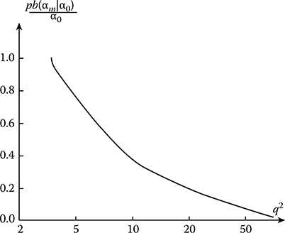
FIGURE 15.9 Relative estimate bias shift as a function of the ratio between the variance of the investigated stochastic process and power noise.

Images

FIGURE 15.10 Relative root-mean-square deviation of estimate as a function of the ratio between the variance of the investigated stochastic process and power noise.

where ρ_en(τ) is the envelope of normalized correlation function and the condition

$2 π Δ f_{ef} < < v (15.167)$

is satisfied. We estimate the parameter ν. In the narrowband stochastic process case, the parameter ν plays a role of the central spectral density frequency. We assume that the stochastic process with the correlation function given by (15.166) is investigated in the white noise with the correlation function

$R_{n} (τ) = \frac{N_{0}}{2} δ (τ), (15.168)$

where δ(τ) is the Dirac delta function and the observation time interval [0, T] is much longer than the correlation stochastic process interval.

In accordance with (15.111), the logarithm of likelihood ratio functional can be presented in the following form:

$M (v) = M_{1} (v) - 0.5 H (v), (15.169)$

where M₁(ν) and H(ν) are given by (15.102) and (15.104), respectively. Consider the second term in (15.169) taking into consideration that

${\begin{array}{l} S_{n} (ω) = \frac{N_{0}}{2}, \\ S_{x} (ω, v) = \frac{1}{2} σ^{2} [ℱ_{1} (ω - v) + ℱ_{1} (ω + v)], \end{array} (15.170)$

where ℱ₁(ω) is the Fourier transform of the normalized correlation function envelope ρ_en(τ). Introducing new variable ω′ = ω - ν and taking into consideration that the investigated stochastic process is the narrowband process, we can write

$H (v) \approx \frac{T}{π} \int_{- \infty}^{\infty} \ln [1 + \frac{σ^{2}}{N_{0}} ℱ_{1} (ω)] d ω = const . (15.171)$

Consequently, the logarithm of likelihood ratio functional accurate with the constant factor coincides with the output signal

$M (v) = T {\int^{}}_{T}^{0} R_{y}^{*} (τ) ϑ (τ; v) d τ . (15.172)$

Taking into consideration (15.106), (15.109), and the fact that the stochastic process ξ(t) is the narrowband process, we obtain

$ϑ (τ; v) = \frac{σ^{2}}{π N_{0}} \int_{- \infty}^{\infty} \frac{[ℱ_{1} (ω - v) + ℱ_{1} (ω + v)] \exp {j ω τ}}{σ^{2} [ℱ_{1} (0) - v) + ℱ_{1} (ω + v)] + N_{0}} d ω = ℱ_{1} (τ) \cos v τ, (15.173)$

where

$ℱ_{1} (τ) = \frac{2 σ^{2}}{π N_{0}} \int_{- \infty}^{\infty} \frac{ℱ_{1} (ω) \exp {j ω τ}}{σ^{2} ℱ_{1} (ω) + N_{0}} d ω . (15.174)$

Thus, the estimation of parameter v can be carried out by position of absolute maximum of the function

$M_{1} (v) = T {\int^{}}_{0}^{T} R_{y}^{*} (τ) {\tilde{ℱ}}_{1} (τ) \cos v τ d τ, (15.175)$

where $R_{y}^{*} (τ)$ is the correlation function estimate of the total process given by (15.103).

Define the bias and variance of estimate of the parameter v limiting only by the first approximation. Under this approximation, the estimate will be unbiased and, in accordance with (15.143) and (15.150), the variance of estimate can be presented in the following form:

$Var {v_{m} | v_{0}} = \frac{2 π}{T σ^{4} {\int^{}}_{- \infty}^{\infty} {\frac{d ℱ_{1} (ω)}{d ω}}^{2} \frac{d ω}{{[σ^{2} ℱ_{1} (ω) + N_{0}]}^{2}}} . (15.176)$

If the normalized correlation function envelope takes the form

$ρ_{en} (τ) = \exp {- α | τ |}, (15.177)$

the Fourier transform can be presented as

$ℱ_{1} (ω) = \frac{2 α}{α^{2} + ω^{2}} . (15.178)$

As a result, the variance of the correlation function parameter estimate takes the following form:

$Var {v_{m} | v_{0}} = α^{2} {(1 + \sqrt{1 + q^{2}})}^{3} \frac{\sqrt{1 + q^{2}}}{q^{4} p}, (15.179)$

where

$q^{2} = \frac{2 σ^{2}}{N_{0} α} . (15.180)$

If q² ≪ 1 and 2σ²T $N_{0}^{- 1}$ ≫ 1, the variance of correlation function parameter estimate is simplified

$Var {v_{m} | v_{0}} = \frac{8 α^{2}}{q^{4} p} . (15.181)$

If q² ≫ 1, then

$Var {v_{m} | v_{0}} = \frac{α^{2}}{p}, (15.182)$

or the variance of the central frequency estimate of stochastic process spectral density is inversely proportional to the product between the correlation interval and observation time interval. Figure 15.11 presents the root-mean-square deviation $\sqrt{p Var {v_{m} | v_{0}} / α^{2}}$ as a function of ratio between the variance of the investigated stochastic process and the power noise q² within the limits of effective spectral bandwidth. In doing so, we assume that for all values of q² the following inequality q²p ≫ 1 is satisfied.

The optimal estimate of stochastic process correlation function can be found in the form of estimations of the elements R_ij of the correlation matrix R or elements C_ij of the inverse matrix C. In the case of Gaussian stationary stochastic process with the multidimensional probability density function given by (12.169), the solution of likelihood ratio equation

$\frac{\partial f_{N} (x_{1}, x_{2}, ..., x_{N} | C)}{\partial C_{i j}} = 0 (15.183)$

allows us to obtain the estimates C_ij and, consequently, the estimates of elements R_ij of correlation matrix R.

Images

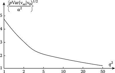
FIGURE 15.11 Relative root-mean-square deviation $\sqrt{p Var {v_{m} | v_{0}} / α^{2}}$ as a function of the ratio between the variance of the investigated stochastic process and power noise.

15.4 Correlation Function Estimation Methods Based on other Principles

Under practical realization of analog correlators based on the estimate given by (15.2), a multiplication of two stochastic processes is most difficult to carry out. We discussed previously that for this purpose there is a need to use the circuits performing a multiplication in accordance with (13.201). The described flowchart consists of two quadrators. There are two methods [1] called the interference and compensation methods using a single quadrator. In doing so, it is assumed that the variance of investigated stochastic process is known very well. The interference method is based on the following relationship:

$R (τ) = \pm {\frac{1}{2} 〈 {[x (t - τ) \pm x (t)]}^{2} 〉 \mp σ^{2}} . (15.184)$

It is natural to use the following function to estimate the correlation function given by (15.184)

$\tilde{R} (τ) = \pm {\frac{1}{2 T} {\int^{}}_{0}^{T} {[x (t - τ) \pm x (t)]}^{2} d t \mp σ^{2}} . (15.185)$

As we can see from (15.184) and (15.185), the estimate of correlation function is not biased.

Let us define the variance of correlation function estimate assuming that the investigated process is Gaussian. Suppose that we use the sign “+” in the square brackets in (15.184) and (15.185). Then

$\begin{array}{l} Var {\tilde{R} (τ)} = & 〈 {\frac{1}{T} {\int^{}}_{0}^{T} x (t) x (t - τ) d t}^{2} 〉 - R^{2} (τ) \\ + \frac{1}{T^{2}} {\int^{}}_{0}^{T} {\int^{}}_{0}^{T} 〈 x (t_{1}) x (t_{1} - τ) [x^{2} (t_{2}) + x^{2} (t_{2} - τ)] 〉 d t_{1} d t_{2} \\ - 2 σ^{2} R (τ) + 〈 {\frac{1}{2 T} {\int^{}}_{0}^{T} [x^{2} (t) + x^{2} (t - τ)] d t}^{2} 〉 - σ^{4} . \end{array} (15.186)$

The first and second terms in the right side of (15.186) represent the variance of the correlation function estimate R*(x) according to (15.2). Other terms on the right side of (15.186) characterize an increase in the variance of the correlation function estimate R*(x) according to (15.185) compared to the estimate given by (15.2). Making mathematical transformations with the introduction of new variables, as it was done earlier, we can write

$\begin{array}{l} Var {\tilde{R} (τ)} = & Var {R^{*} (τ)} + \frac{1}{T} {\int^{}}_{0}^{T} (1 - \frac{τ}{T}) \\ \times {2 R^{2} (z) + R^{2} (z + τ) + R^{2} (z - τ) + 4 R (z) [R (z + τ) + R (z - τ)]} d z . \end{array} (15.187)$

As τ → 0

$Var {\tilde{R} (0)} \approx \frac{16}{T} {\int^{}}_{0}^{T} 1 - \frac{τ}{T} R^{2} (z) d z, (15.188)$

and, in this case, the variance of correlation function estimate given by (15.185) exceeds by four times the variance of correlation function estimate given by (15.2).

If the condition. T ≫ τ_cor is satisfied, the variance of correlation function estimate given by (15.185) can be presented in the following form:

$\begin{array}{l} Var {\tilde{R} (τ)} = & \frac{2}{T} {\int^{}}_{0}^{\infty} [R^{2} (z) + R (z + τ) R (z - τ)] d z \\ + \frac{1}{T} {\int^{}}_{0}^{T} {2 R^{2} (z) + R^{2} (z + τ) + R^{2} (z - τ) + 4 R (z) [R (z + τ) + R (z - τ)]} d z . \end{array} (15.189)$

At T ≫ τ ≫ τ_cor, we have

$Var {\tilde{R} (τ)} \approx \frac{6}{T} {\int^{}}_{0}^{\infty} R^{2} (z) d z . (15.190)$

Under accepted initial conditions, we obtain

${\int^{}}_{0}^{\infty} R^{2} (z - τ) d z \approx {\int^{}}_{0}^{\infty} R^{2} (υ) d υ = 2 {\int^{}}_{0}^{\infty} R^{2} (υ) d υ . (15.191)$

As applied to the exponential correlation function given by (12.13) and if the condition T ≫ τ_cor is satisfied, the variance of correlation function estimate given by (15.185) can be written in the following form:

$Var {\tilde{R} (τ)} = \frac{σ^{4}}{α T} [3 + 4 (1 + α T) \exp {- α T} + (1 + 2 α T) \exp {- 2 α T}] . (15.192)$

Using the compensation method to measure the correlation function, the function

$μ (τ, γ) = 〈 {[x (t - τ) - γ x (t)]}^{2} 〉 (15.193)$

is formed and a selection of the factor γ ensuring a minimum of the function μ(τ, γ) is performed. In doing so, the factor γ becomes numerically equal to the normalized correlation function value. Thus, likelihood defining the minimum of the function μ(τ, γ) based on the condition

$\begin{matrix} \frac{d μ (τ, γ)}{d γ} = 0 & if & \frac{d^{2} μ (τ, γ)}{d γ^{2}} > 0, \end{matrix} (15.194)$

we obtain

$γ = \frac{〈 x (t) x (t - τ) 〉}{〈 x^{2} (t) 〉} = ℛ (τ) . (15.195)$

Consequently, the compensation measurer of correlation function should generate the function of the following form:

$μ^{*} (τ, γ) = \frac{1}{T} {\int^{}}_{0}^{T} {[x (t - τ) - γ x (t)]}^{2} d t . (15.196)$

Minimizing the function μ*(τ, γ) given by (15.196) with respect to the parameter γ, we are able to obtain the estimate of normalized correlation function γ = ℛ(τ). Solving the equation

$\frac{d μ^{*} (τ, γ)}{d γ} = 0, (15.197)$

we can see that the procedure to define the estimate of the correlation function R*(τ) is equivalent to the estimate that can be presented in the following form:

$γ^{*} = \tilde{ℛ} (τ) = \frac{(1 / T) {\int^{}}_{0}^{T} x (t) x (t - τ) d t}{(1 / T) {\int^{}}_{0}^{T} x^{2} (t) d t} . (15.198)$

As was shown in Ref. [1], as applied to the estimate by minimum of the function μ(τ, γ) given by (15.196), the requirements of quadrator are less stringent compared to the requirements of quadrators used by the previously discussed methods of correlation function measurement.

Determine the statistical characteristics of normalized correlation function estimate of the Gaussian stochastic process. For this purpose, we present the numerator and denominator in (15.198) in the following form:

$\frac{1}{T} {\int^{}}_{0}^{T} x (t) x (t - τ) d t = σ^{2} ℛ (τ) + σ^{2} Δ ℛ (τ) . (15.199)$

$\frac{1}{T} {\int^{}}_{0}^{T} x^{2} (t) d t = σ^{2} [1 + \frac{Δ Var}{σ^{2}}] . (15.200)$

As discussed earlier,

$〈 Δ ℛ (τ) 〉 = 0, (15.201)$

$〈 Δ Var 〉 = 0. (15.202)$

Their variances are given by (15.9) and (13.62), respectively. Henceforth, we assume that the condition T ≫ τ_cor is satisfied. In this case, the error of variance estimate is negligible compared to the true value of variance

$\frac{〈 {(Δ Var)}^{2} 〉}{σ^{4}} ≪ 1. (15.203)$

Because of this, we can use the following approximation of estimate given by (15.198)

$\tilde{ℛ} (τ) = \frac{ℛ (τ) + Δ ℛ (τ)}{1 + (Δ Var / σ^{2})} \approx ℛ (τ) + Δ ℛ (τ) [1 - \frac{Δ V a r}{σ^{2}} + {(\frac{Δ Var}{σ^{2}})}^{2}] . (15.204)$

Under the definition of the bias and variance of estimate, a limitation is imposed by the terms containing the moments of random variables Δℛ(τ) and ΔVar/σ², and the order of these terms is not higher than 2. Under this approximation, the mathematical expectation of estimate of the normalized correlation function (15.204) can be presented in the following form:

$〈 〈 \tilde{ℛ} (τ) 〉 〉 = ℛ (τ) - \frac{〈 Δ ℛ (τ) Δ Var 〉}{σ^{2}} + ℛ (τ) {(\frac{Δ Var}{σ^{2}})}^{2} . (15.205)$

Thus, the estimate of the normalized correlation function given by (15.198) is characterized by the bias

$b [\tilde{ℛ} (τ)] = 〈 \tilde{ℛ} (τ) 〉 - ℛ (τ) = - \frac{〈 Δ ℛ (τ) Δ Var 〉}{σ^{2}} + ℛ (τ) {(\frac{Δ Var}{σ^{2}})}^{2} . (15.206)$

The product moment 〈Δℛ(τ)ΔVar〉 can be presented in the following form:

$\begin{array}{l} 〈 Δ ℛ (τ) Δ Var 〉 & = 〈 {\frac{1}{σ^{2} T} {\int^{}}_{0}^{T} x (t) x (t - τ) d t - ℛ (τ)} \times {\frac{1}{T} {\int^{}}_{0}^{T} x^{2} (t) d t - σ^{2}} 〉 \\ = \frac{1}{σ^{2} T} {\int^{}}_{0}^{T} {\int^{}}_{0}^{T} 〈 x (t_{1}) x (t_{1} - τ) x^{2} (t_{2}) 〉 d t_{1} d t_{2} - σ^{2} ℛ (τ) . \end{array} (15.207)$

Determining the fourth product moment and making transformations and introducing new variables under the condition T ≫ τ_cor, as it was done before, we can write

$\frac{〈 Δ ℛ (τ) Δ V a r 〉}{σ^{2}} = \frac{2}{T} {\int^{}}_{0}^{\infty} ℛ (z) [ℛ (z + τ) + ℛ (z - τ)] d z . (15.208)$

Taking into consideration (15.208) and the variance of variance estimate given by (13.63), we obtain the estimate bias in the following form:

$b [\tilde{ℛ} (τ)] = - \frac{2}{T} {\int^{}}_{0}^{\infty} ℛ (z) [ℛ (z + τ) + ℛ (z - τ)] d z + ℛ (z) \frac{4}{T} {\int^{}}_{0}^{T} ℛ^{2} (z) d z . (15.209)$

To define the variance of the normalized correlation function estimate

$V a r {\tilde{ℛ} (τ)} = 〈 {\tilde{ℛ}}^{2} (τ) 〉 - {[〈 \tilde{ℛ} (τ) 〉]}^{2} (15.210)$

we determine $〈 {\tilde{ℛ}}^{2} (τ) 〉$ accurate with the terms of the moments $Δ ℛ (τ)$ and ΔVar of the second order

$〈 {\tilde{ℛ}}^{2} (τ) 〉 = 〈 \frac{{[ℛ (τ) + Δ ℛ (τ)]}^{2}}{[1 + {(Δ V a r / σ^{2}]}^{2}} 〉 \approx 〈 {ℛ^{2} (τ) + 2 ℛ (τ) Δ ℛ (τ) + {[Δ ℛ (τ)]}^{2}} {1 - 2 \frac{Δ V a r}{σ^{2}} + 3 {(\frac{Δ V a r}{σ^{2}})}^{2}} 〉 \approx ℛ^{2} (τ) + 〈 Δ ℛ^{2} (τ) 〉 + 3 ℛ^{2} (τ) \frac{〈 {(Δ V a r)}^{2} 〉}{σ^{4}} - 4 ℛ (τ) \frac{〈 Δ V a r Δ ℛ (τ) 〉}{σ^{2}} . (15.211)$

Taking into consideration (15.205) and the earlier-given moments, we obtain

$V a r {\tilde{ℛ} (τ)} = \frac{2}{T} {\int^{}}_{0}^{\infty} [ℛ^{2} (z) + ℛ (z + τ) ℛ (z - τ)] d z + ℛ^{2} (τ) \frac{4}{T} {\int^{}}_{0}^{T} ℛ^{2} (z) d z - ℛ (τ) \times \frac{4}{T} {\int^{}}_{0}^{\infty} ℛ (z) [ℛ (z + τ) + ℛ (z - τ)] d z . (15.212)$

As we can see from (15.209) and (15.212), as τ → 0 the bias and variance of estimate given by (15.198) tend to approach zero, since at τ = 0, according to (15.198), the normalized correlation function estimate is not a random variable.

As applied to the Gaussian stochastic process with the exponential correlation function given by (12.13), the bias and variance of the normalized correlation function estimate take the following form:

$b [\tilde{ℛ} (τ)] = - \frac{2}{T} \exp {- α τ}, (15.213)$

$V a r {\tilde{ℛ} (τ)} = \frac{1}{T α} [1 - (1 + 2 α τ) \exp {- 2 α τ}] . (15.214)$

The sign or polar methods of measurements allow us to simplify essentially the experimental investigation of correlation and mutual correlation functions. Delay and multiplication of stochastic processes can be realized very simply by circuitry. The sign methods of correlation function measurements are based on the existence of a functional relationship between the correlation functions of the initial stochastic process ξ(t) and the transformed stochastic process η(t) = sgn ξ(t). The stochastic process η(t) is obtained by nonlinear inertialess transformation of initial stochastic process ξ(t) by the ideal two-sided limiter with transformation characteristic given by (12.208).

As applied to the Gaussian stochastic process, its normalized correlation function $ℛ (t)$ is related to the correlation function ρ(τ) of the transformed stochastic process η(t) = sgn ξ(t) by the following relationship:

$ℛ (τ) = \sin [0.5 π ρ (τ)] = - \cos [2 π P_{+} (τ)], (15.215)$

where

$P_{+} (τ) = {\int^{}}_{0}^{\infty} {\int^{}}_{0}^{\infty} p_{2} (x_{1}, x_{2}; τ) d x_{1} d x_{2} (15.216)$

is the probability of coincidence between the positive signs of functions η(t) and η(t − τ). The estimate of the probability P₊(τ) can be obtained as a signal averaging by time at the matching network output of positive values of the stochastic functions η(t) and η(t − τ) realizations. If the stochastic process is non-Gaussian, a relationship between the correlation functions of initial and transformed by the ideal limiter stochastic processes is very complex. For this reason, the said method of correlation function measurement is restricted. The method of correlation function measurement using additional processes by analogy with the discussed method of estimation of the mathematical expectation and variance of stochastic process is widely used.

Assume that the investigated stochastic process η(t) has zero mathematical expectation. Consider two sign functions

${_{η_{2} (t - τ) = s g n [ξ (t - τ) - μ_{2} (t - τ)]}^{η_{1} (t) = s g n [ξ (t) - μ_{1} (t)]}, (15.217)$

where the mutual independent additional stationary stochastic processes μ₁(t) and (μ₂t) have the same uniform probability density functions given by (12.205) and the condition (12.206) is satisfied. As mentioned previously, the conditional stochastic processes η₁(t|x₁) and η₂[(t − τ)|x₂] are mutually independent at the fixed values ξ(t) = x₁ and η(t − τ) = x₂. Taking into consideration (12.209), we obtain

$〈 η_{1} (t | x_{1}) η_{2} [(t - τ) | x_{2}] 〉 = \frac{x_{1} x_{2}}{A^{2}} . (15.218)$

The unconditional mathematical expectation of product between two stochastic functions can be presented in the following form:

$〈 η_{1} (t) η_{2} (t) 〉 = \frac{1}{A^{2}} \int_{- \infty}^{\infty} \int_{\infty}^{\infty} x_{1} x_{2} p_{2} (x_{1}, x_{2}; τ) d x_{1} d x_{2} = \frac{R (τ)}{A^{2}} . (15.219)$

Thus, the function

$\tilde{ℛ} (τ) = \frac{A^{2}}{N} {\sum^{}}_{i = 1}^{N} y_{1 i} y_{2 i}, (15.220)$

where y_1i and y_2i are the samples of stochastic sequences η_i₁ and η_2i, can be considered as the estimate of correlation function to be used for the investigation of stochastic process at discrete instants. In this case, the estimate will be unbiased. When additional stochastic functions are carried out to estimate the variance (see Section 13.3), the operations of product and summation in (15.220) are easily changed by operations of defnition of estimate difference between the probability of polarity coincidence and noncoincidence of sampled values y₁_i and y_2i. Delay operations of sign functions can be implemented by circuitry.

Determine the variance of correlation function estimate given by (15.220) assuming that the samples are pairwise independent, that is,

$〈 y_{1 i} y_{1 j} 〉 = 〈 y_{2 i} y_{2 j} 〉 = 0 (15.221)$

we obtain

$V a r {\tilde{R} (τ)} = \frac{A^{4}}{N^{2}} {\sum^{}}_{i = 1}^{N} {\sum^{}}_{j = 1}^{N} 〈 y_{1 i} y_{2 i} y_{1 j} y_{2 j} 〉 - R^{2} (τ) . (15.222)$

The double sum can be presented in the form of two sums by analogy with (13.94). At this time, (13.55) is true. Define the conditional product moment 〈(η_1iη_1jη_2j| x_1i, x_2i, x_1j, x_2j)〉 if i ≠ j under the condition

${\begin{cases} ξ (t_{i} - τ) = x_{1 i}, \\ ξ (t_{i} - τ) = x_{2 i,} \\ ξ (t_{j}) = x_{1 j}, \\ ξ (t_{j} - τ) = x_{2 i} . \end{cases} (15.223)$

Taking into consideration a statistical independence between η₁ and η₂, mutual independence between the conditional random values η₁(t_i|x₁_i ) and η₂ [(t_i − τ)|x_2i], and (12.209), the conditional product moment can be written in the following form:

$〈 (η_{1 i} η_{2 i} η_{1 j} η_{2 j} | x_{1 i}, x_{2 i}, x_{1 j}, x_{2 j}) 〉 = \frac{x_{1 i} x_{2 i} x_{1 j} x_{2 j}}{A^{4}} . (15.224)$

Given that the random variables η_i and η_j are independent of each other, the unconditional product moment can be presented in the following form:

$〈 η_{1 i} η_{2 i} η_{1 j} η_{2 j} 〉 = \frac{1}{A^{4}} {\int_{- \infty}^{\infty} \int_{- \infty}^{\infty} x_{1} x_{2} p_{2} (x_{1}, x_{2}; τ) d x_{1} d x_{2}}^{2} = \frac{R^{2} (τ)}{A^{4}} . (15.225)$

Substituting (13.96) and (15.225) into (13.94) and then into (15.222), we obtain

$V a r {\tilde{R} (τ)} = \frac{A^{4}}{N} [1 - \frac{R^{2} (τ)}{A^{4}}] . (15.226)$

According to (15.220), the correlation function estimate satisfies the condition given by (12.206), that is, σ² ≪ A². For this reason, the variance of correlation function estimate is defined by half-intervals of possible values of additional stochastic processes. Comparing (15.226) and (15.25), we obtain

$\frac{V a r {\tilde{R} (τ)}}{V a r {R^{*} (τ)}} = \frac{A^{4}}{σ^{4}} \times \frac{1 - (σ^{4} / A^{4}) ℛ^{2} (τ)}{1 + ℛ^{2} (τ)} . (15.227)$

As we can see from (15.227), since the condition σ² ≪ A² is satisfied, the correlation function estimate given by (15.220) is worse compared to the correlation function estimate given by (15.21).

15.5 Spectral Density Estimate Of Stationary Stochastic Process

By defnition, the spectral density of stationary stochastic process is the Fourier transform of correlation function

$S (ω)) = \int_{- \infty}^{\infty} R (τ) \exp {- j 0) τ} d τ . (15.228)$

The inverse Fourier transform takes the following form:

$R (τ) = \frac{1}{2 π} \int_{- \infty}^{\infty} S (ω) \exp {j ω τ} d ω . (15.229)$

As we can see from (15.229), at τ = 0 we obtain the variance of stochastic process:

$V a r = R (τ = 0) = \frac{1}{2 π} \int_{- \infty}^{_{\infty}} S (ω) d ω . (15.230)$

As applied to the ergodic stochastic process with zero mathematical expectation, the correlation function is defined by (15.1). Because of this, we can rewrite (15.1) in the following form:

$S_{1} (0)) = \lim_{T \to \infty} \frac{1}{T} {\int^{}}_{0}^{T} x (t) {\int_{- \infty}^{\infty} x (t - τ) \exp {- j ω τ} d τ} d t . (15.231)$

The received realization of stochastic process can be presented in the following form:

$x (t) = {_{0 i f [t] > T .}^{x (t) i f 0 \leq t \leq T,} (15.232)$

In the case of physically realized stochastic processes, the following condition is satisfied:

${\int^{}}_{0}^{T} x^{2} (t) d t = \int_{- \infty}^{\infty} x^{2} (t) d t < \infty (15.233)$

For the realization of the stochastic process, the Fourier transform takes the following form:

$X (j ω) = {\int^{}}_{0}^{T} x (t) \exp {- j ω τ} d t = \int_{- \infty}^{\infty} x (t) \exp {- j ω τ} d t . (15.234)$

Introducing a new variable z = t − τ, we can write

$\int_{- \infty}^{\infty} x (t - τ) \exp {- j ω τ} d τ = X (- j ω) \exp {- j ω τ} . (15.235)$

Substituting (15.235) into (15.231) and taking into consideration (15.234), we obtain

$S_{1} (ω) = \lim_{T \to \infty} \frac{1}{T} | X (j ω) |^{2} . (15.236)$

Formula (15.236) is not correct for the defnition of spectral density as the characteristic of stochastic process averaged in time. This phenomenon is caused by the fact that the function T^-1|X(jω)|² is the stochastic function of the frequency ω. As the stochastic function x(t), this function changes randomly by its mathematical expectation and possesses the variance that does not tend to approach zero with an increase in the observation time interval. Because of this, to obtain the averaged characteristic corresponding to the defnition of spectral density according to (15.228), the spectral density S1(ω) should be averaged by a set of realizations of the investigated stochastic process and we need to consider the function

$S (ω) = \lim_{\begin{array}{l} T \to \infty \\ N \to \infty \end{array}} \frac{1}{T} {\sum^{}}_{i = 1}^{N} | X_{j} (j ω) |^{2} . (15.237)$

Consider the statistical characteristics of estimate of the function

$S_{1}^{*} (ω) = \frac{|_{X_{i} (j ω)} |^{2}}{T}, (15.238)$

where the random spectrum X(jω) of stochastic process realization is given by (15.234).

The mathematical expectation of spectral density estimate given by (15.238) takes the following form:

$\begin{array}{l} {S_{1}^{*} (ω)} = \frac{〈 |_{X_{i} (j ω)} |^{2} 〉}{T} = \frac{1}{T} {\int^{}}_{0}^{T} {\int^{}}_{0}^{T} 〈 x (t_{1}) x (t_{2}) 〉 \exp {- j ω (t_{2} - t_{l}} d t_{l} d t_{2} \\ = \frac{1}{T} {\int^{}}_{0}^{T} {\int^{}}_{0}^{T} R (t_{2} - t_{1}) \exp {- j ω (t_{2} - t_{1})} d t_{1} d t_{2} . \end{array} (15.239)$

After introduction of new variables τ = t₂.- t₁.and t₂ = t, the double integral in (15.239) can be transformed into a single integral, that is,

$〈 S_{1}^{*} (ω) 〉 = {\int^{}}_{- T}^{T} (1 - \frac{| τ |}{T}) R (τ) \exp {- j ω τ} d τ . (15.240)$

If the condition T ≫ τ_cor is satisfied, we can neglect the second term compared to the unit in paren-thesis in (15.240), and the integration limits are propagated on ±∞. Consequently, as T → ∞, we can write

${S_{1}^{*} (ω)} = S (ω) . (15.241)$

that is, as T → ∞, the spectral density estimate of stochastic process is unbiased.

Determine the correlation function of spectral density estimate

$\begin{array}{l} R (ω_{1,} ω_{2}) = 〈 S_{1}^{*} (ω_{1}) S_{1}^{*} (ω_{2}) 〉 - 〈 S_{1}^{*} (ω_{1}) S_{1}^{*} (ω_{2}) 〉 〈 S_{1}^{*} (ω_{2}) 〉 \\ = \frac{1}{T^{2}} {\int^{}}_{0}^{T} {\int^{}}_{0}^{T} {\int^{}}_{0}^{T} {\int^{}}_{0}^{T} 〈 x (t_{1}) x (t_{2}) x (t_{3}) x (t_{4}) 〉 \exp {- j ω_{1} t_{1} + j ω_{1} t_{2} - j ω_{2} t_{3} + j ω_{2} t_{4}} d t_{1} d t_{2} d t_{3} d t_{4} \\ - \frac{1}{T^{2}} {\int^{}}_{0}^{T} {\int^{}}_{0}^{T} 〈 x (t_{1}) x (t_{2}) 〉 \exp {- j ω_{1} t_{1} + j ω_{1} t_{2}} d t_{1} d t_{2} \\ \times {\int^{}}_{0}^{T} {\int^{}}_{0}^{T} 〈 x (t_{3}) x (t_{4}) 〉 \exp {- j ω_{2} t_{3} + j ω_{2} t_{4}} d t_{3} d t_{4} \end{array} (15.242)$

As applied to the Gaussian stochastic process, (15.242) can be reduced to

$R (ω_{1}, ω_{2}) = \frac{1}{T^{2}} {\int^{}}_{0}^{T} {\int^{}}_{0}^{T} {\int^{}}_{0}^{T} {\int^{}}_{0}^{T} [R (t_{1} - t_{3}) R (t_{2} - t_{4}) + R (t_{1} - t_{4}) R (t_{2} - t_{3})] \times \exp {- j ω_{1} t_{1} + j ω_{1} t_{2} - j ω_{2} t_{3} + j ω_{2} t_{4}} d t_{1} d t_{2} d t_{3} d t_{4} . (15.243)$

Taking into consideration (15.229) and (12.122) and as T → ∞, we obtain

$\begin{array}{l} R (ω_{1}, ω_{2}) = \frac{S (ω_{1}) S (ω_{2})}{T^{2}} {{\int^{}}^{}_{T}^{0} \exp {- j (ω_{1} + ω_{2})} t d t {\int^{}}^{}_{T}^{0} \exp {j (ω_{1} + ω_{2})} t d t + {\int^{}}^{}_{T}^{0} \exp {- j (ω_{1} - ω_{2})} t d t {\int^{}}^{}_{T}^{0} \exp {j (ω_{1} - ω_{2})} t d t} \\ = S (ω_{1}) S (ω_{2}) {[\frac{2 \sin \frac{ω_{1} + ω_{2}}{2} T}{(ω_{1} + ω_{2}) T}] 2 + [\frac{2 \sin \frac{ω_{1} - ω_{2}}{2} T}{(ω_{1} - ω_{2}) T}] 2} . \end{array} (15.244)$

If the condition ωT ≫ 1 is satisfied, we can use the following approximation:

$R (ω_{1}, ω_{2}) \approx S (ω_{1}) S (ω_{2}) {\frac{\sin [0.5 (ω_{1} - ω_{2}) T]}{0.5 (ω_{1} - ω_{2}) T}}^{2} . (15.245)$

$ω_{1} - ω_{2} = \frac{2 i π}{T}, i = 1, 2, ..., (15.246)$

then

$R (ω_{1}, ω_{2}) = 0, (15.247)$

which means, if the frequencies are detuned on the value multiple 2πT^-1, the spectral components $S_{1}^{*} (ω_{1}) a n d S_{i}^{*} (ω_{2})$ are uncorrelated. When 0.5(ω₁ - ω₂) T ≫ 1, we can neglect the correlation function between the estimates of spectral density given by (15.238).

The variance of estimate of the function S((ω₁) can be defined by (15.244) using the limiting case at ω₁ = ω₂ = ω:

$V a r {S_{1}^{*} ω} = S^{2} (ω) {\frac{\sin^{2} ω T}{{(ω T)}^{2}} + 1} . (15.248)$

If the condition ωT ≫ 1 is satisfied (as T → ∞), we obtain

$\lim_{T \to \infty} V a r {S_{1}^{*} (ω)} = S^{2} (ω) . (15.249)$

Thus, according to (15.238), in spite of the fact that the estimate of spectral density ensures unbi-asedness, it is not acceptable because the value of the estimate variance is larger than the squared spectral density true value.

Averaging the function $S_{1}^{*} (ω)$ by a set of realizations is not possible, as a rule. Some indirect methods to average the function $S_{1}^{*} (ω)$ are discussed in Refs. [3,5,6]. The first method is based on implementation of the spectral density averaged by frequency bandwidth instead of the estimate of spectral density defined at the point (the estimate of the given frequency). In doing so, the more the frequency range, within the limits of which the averaging is carried out, at T = const, the lesser the variance of estimate of spectral density. However, as a rule, there is an estimate bias that increases with an increase in the frequency range, within the limits of which the averaging is carried out. In general, this averaged estimate of spectral density can be presented in the following form:

$s_{2}^{*} (ω) = \frac{1}{2 π} \int_{- \infty}^{\infty} W (ω) S_{1}^{*} (ω - v) d v, (15.250)$

where W(ω) is the even weight function of frequency ω or as it is called in other words the function of spectral window. The widely used functions W(ω) can be found in Refs. [3,5,6].

As T → ∞, the bias of spectral density estimate $S_{2}^{*} (ω)$ can be presented in the following form:

$b {S_{2}^{*} (ω)} = \frac{1}{2 π} \int_{- \infty}^{\infty} S (ω - ν) W (ω) d ν - S (ω) . (15.251)$

As applied to the narrowband spectral window W(ω), the following expansion

$S (ω - ν) \approx S (ω) - S^{'} (ω) + 0. 5^{″} (ω) ν^{2} (15.252)$

is true, where S′(ω) and S″(ω) are the derivatives with respect to the frequency ω. Because of this, we can write

$b {S_{2}^{*} (ω)} \approx \frac{S^{″} (ω)}{4 π} \int_{- \infty}^{\infty} ω^{2} W (ω) d ω . (15.253)$

If the condition ωT ≫ 1 is satisfied (as T → ∞), we obtain [1]

$V a r {S_{2}^{*} (ω)} \approx \frac{S^{2} (ω)}{2 π T} \int_{- \infty}^{\infty} W^{2} (ω) d ω . (15.254)$

As we can see from (15.254), as T → ∞, $Var {S_{2}^{*} (ω)} \to 0$ ; that is, the estimate of the spectral density $S_{2}^{*} (ω)$ is consistent.

The second method to obtain the consistent estimate of spectral density is to divide the observation time interval [0, T] on N subintervals with duration T₀ < T and to define the estimate $S_{1 i}^{*} (ω)$ for each subinterval and subsequently to determine the averaged estimate

$S_{3}^{*} (ω) = \frac{1}{N} \sum_{i = 1}^{N} S_{1 i}^{*} (ω), N = \frac{T}{T_{0}} . (15.255)$

Note that according to (15.240), at T = const, an increase in N(or decrease in T₀) leads to bias of the estimate $S_{3}^{*} (ω)$ . If the condition T₀ ≫ τ_cor is satisfied, the variance of estimate $S_{3}^{*} (ω)$ can be approximated by the following form:

$V a r {S_{3}^{*} (ω)} \approx \frac{S^{2} (ω)}{N} . (15.256)$

As we can see from (15.256), as T → ∞, the estimate given by (15.255) will be consistent.

In radar applications, sometimes it is worthwhile to obtain the current estimate $S_{1}^{*} (ω, t)$ instead of the averaged summation given by (15.225). Subsequently, the obtained function of time is smoothed by the low-pass filter with the filter constant time τ_filter ≫ T₀. This low-pass filter is equivalent to estimate by ν uncorrelated estimations of the function $S_{1}^{*} (ω)$ , where $v = τ_{filter} T_{0}^{- 1}$ . In practice, it makes sense to consider only the positive frequencies f = ω(2π)⁻¹. Taking into consideration that the correlation function and spectral density remain even, we can write

$G (f) = 2 S (ω = 2 π f), f > 0. (15.257)$

According to (15.228) and (15.229), the spectral density G(f) and the correlation function R(x) take the following form:

$G (f) = 4 \int_{0}^{\infty} R (τ) \cos 2 π f τ d τ, (15.258)$

$R (τ) = \int_{0}^{\infty} G (f) \cos 2 π f τ d f . (15.259)$

In this case, the current estimate, by analogy with (15.238), can be presented in the following form:

$G_{1}^{*} (f, t) = \frac{2 A^{2} (f, t)}{T_{0}}, (15.260)$

where the squared current spectral density can be presented in the following form:

$A^{2} (f, t) = {| X (j ω, t) |}^{2} = A_{c}^{2} (f, t) + A_{s}^{2} (f, t) = {\int_{t - T_{0}}^{t} x (t) \cos 2 π f t d t}^{2} + {\int_{t - T_{0}}^{t} x (t) \sin 2 π f t d t}^{2}, (15.261)$

where $A_{c}^{2} (f, t)$ and $A_{s}^{2} (f, t)$ are the cosine and sine components of the current spectral density of realization x(t). As a result of smoothing the estimate $G_{1}^{*} (f, t)$ by the filter with the impulse response h(t), we can write the averaged estimate of spectral density in the following form:

$G_{2}^{*} (f, t) = \int_{0}^{\infty} h (z) G_{1}^{*} (f, t - z) d z . (15.262)$

$h (t) = α_{0} \exp {- α_{0} t}, t > 0, τ_{f i l t e r} = \frac{1}{α_{0}}, (15.263)$

the variance of spectral density estimate $G_{2}^{*} (f, t)$ can be approximated by

$V a r {G_{2}^{*} (f, t)} \approx \frac{G^{2} (f)}{α_{0} T_{0}} . (15.264)$

The flowchart illustrating how to define the current estimate $G_{2}^{*} (f, t)$ of spectral density is shown in Figure 15.12. The input realization of stochastic process is multiplied by the sine and cosine signals of the reference generator in quadrature channels, correspondingly. Obtained products are integrated, squared, and come in at the summator input. The current estimate $G_{2}^{*} (f, t)$ forming at the summator output comes in at the smoothing filter input. The smoothing filter possesses the impulse response h(t). The smoothed estimate G(f, t) of spectral density is issued at the filter output.

Images

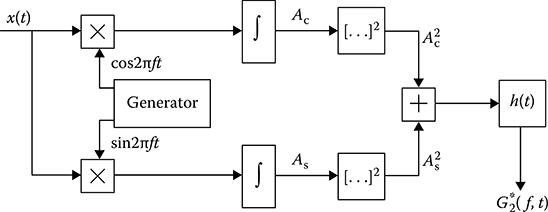
FIGURE 15.12 Defnition of the current estimate of spectral density.

To measure the spectral density within the limits of whole frequency range we need to change the reference generator frequency discretely or continuously, for example, by the linear law.

In practice, the filtering method is widely used. The essence of filtering method is the following. The investigated stationary stochastic process is made to pass through the narrowband (compared to the stochastic process spectrum bandwidth) filter with the central frequency ω₀ = 2πf₀. The ratio between the variance of stochastic process at the narrowband filter output and the bandwidth Δf of the filter is considered as the estimate of spectral density of stochastic process.

Let h(t) be the impulse response of the narrowband filter. The transfer function corresponding to the impulse response h(t) is ℋ(jω). The stationary stochastic process forming at the filter output takes the form:

$y (t, ω_{0}) = \int_{0}^{\infty} h (t - τ) x (τ) d τ . (15.265)$

Spectral density $\tilde{G} (f)$ at the filter output can be presented in the following form:

$\tilde{G} (f) = G (f) ϰ^{2} (f), (15.266)$

where ℋ(f) is the filter transfer function module with the maximum defined as ℋ_max(f) = ℋ_max. The narrowband filter bandwidth can be defined as

$Δ f = \int_{0}^{\infty} \frac{ϰ^{2} (f)}{ϰ_{\max}^{2}} d f . (15.267)$

The variance of stochastic process at the filter output in stationary mode takes the following form:

$V a r {y (t, f_{0})} = 〈 y^{2} (t, f_{0}) 〉 = \int_{0}^{\infty} G (f) ϰ^{2} (f) d f . (15.268)$

Assume that the filter transfer function module is concentrated very closely about the frequency f₀ and we can think that the spectral density is constant within the limits of the bandwidth Δf, that is, G(f) ≈ G(f₀). Then

$V a r {y (t, f_{0})} \approx G (f_{0}) Δ f ϰ_{\max}^{2} . (15.269)$

Naturally, the accuracy of this approximation increases with concomitant decrease in the filter bandwidth Δf, since as Δf → 0 we can write

$G (f_{0}) = \lim_{△ f \to 0} \frac{V a r {y (t, f_{0})}}{Δ f ϰ_{\max}^{2}} . (15.270)$

As applied to the ergodic stochastic processes, under defnition of variance, the averaging by realization can be changed based on the averaging by time as T → ∞

$G (f_{0}) = \lim_{\underset{T \to \infty}{△ f \to 0}} \frac{1}{T Δ f ϰ_{\max}^{2}} \int_{0}^{T} y^{2} (t, f_{0}) d t . (15.271)$

For this reason, the value

$G^{*} (f_{0}) = \frac{1}{T Δ f ϰ_{\max}^{2}} \int_{0}^{T} y^{2} (t, f_{0}) d t (15.272)$

is considered as the estimate of spectral density under designing and construction of measurers of stochastic process spectral density. The values Δf and $ℋ_{\max}^{2}$ are known before. Because of this, a measurement of the stochastic process spectral density is reduced to estimate of stochastic process variance at the filter output. We need to note that (15.272) envisages a correctness of the condition TΔf ≫1, which means the observation time interval is much longer compared to the narrowband filter time constant.

Based on (15.272), we can design the flowchart of spectral density measurer shown in Figure 15.13. The spectral density value at the fixed frequency coincides accurately within the constant factor with the variance of stochastic process at the filter output with known bandwidth. Operation principles of the spectral density measurer are evident from Figure 15.13. To define the spectral density for all possible values of frequencies, we need to design the multichannel spectrum analyzer and the central frequency of narrowband filter must be changed discretely or continuously. As a rule, a shift by spectrum frequency of investigated stochastic process needs to be carried out using, for example, the linear law of frequency transformation instead of filter tuning by frequency. The structure of such measurer is depicted in Figure 15.14. The sawtooth generator controls the operation of measurer that changes the frequency of heterodyne.

Images

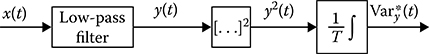
FIGURE 15.13 Measurement of spectral density.

Images

FIGURE 15.14 Measurement of spectral density by spectrum frequency shift.

Define the statistical characteristics for using the filter method to measure the spectral density of stochastic process according to (15.272). The mathematical expectation of spectral density estimate at the frequency f₀ takes the following form:

${G^{*} (f_{0})} = \frac{〈 y^{2} (t, f_{0}) 〉}{Δ f ϰ_{\max}^{2}} = \frac{1}{Δ f ϰ_{\max}^{2}} {\int^{}}_{\infty}^{0} G (f) ϰ^{2} (f) d f . (15.273)$

In a general case, the estimate of spectral density will be biased, that is,

$b {G_{0} (f)} = 〈 G^{*} (f_{0}) 〉 - G (f_{0}) . (15.274)$

The variance of spectral density estimate is defined by the variation in the variance estimate of stochastic process y(t,f₀) at the filter output. If the condition T ≫ τ_cor is satisfied for the stochastic process y(t,f₀), the variance of estimate is given by (13.64), where instead of S(ω) we should understand

$S_{y} (ω) = | ϰ (j ω) |^{2} S (ω) . (15.275)$

As applied to introduced notations G(f) and ℋ(f), we can write

$V a r {G^{*} (f_{0})} = \frac{1}{T {(Δ f)}^{2} ϰ_{\max}^{4}} {\int^{}}_{\infty}^{0} G^{2} (f) ϰ^{4} (f) d f . (15.276)$

To define the bias and variance of spectral density estimate of stochastic process we assume that the module of transfer function is approximated by the following form:

$ϰ (f) = {\begin{matrix} ϰ_{\max}, f_{0} - 0.5 Δ f \leq f \leq f_{0} + 0.5 Δ f; \\ 0, f_{0} - 0.5 Δ f > f, f_{0} + 0.5 Δ f < f, \end{matrix} (15.277)$

where Δf = δf. We apply an expansion in power series about the point. f = f₀ for the spectral density G(f) and assume that there is a limitation imposed by the first three terms of expansion in series, namely,

$G (f) \approx G (f_{0}) + G' (f_{0}) (f - f_{0}) + 0.5 G' (f_{0}) (f - f_{0})^{2}, (15.278)$

where G′(f₀) and G″(f₀) are the first and second derivatives with respect to the frequency f at the point f₀. Substituting (15.278) and (15.277) into (15.273) and (15.274), we obtain

$b {G^{*} (f_{0})} \approx \frac{1}{24} (Δ f)^{2} G^{″} (f_{0}) . (15.279)$

Thus, the bias of spectral density estimate of stochastic process is proportional to the squared bandwidth of narrowband filter. To define the variance of estimate for the first approximation, we can assume that the condition G(f) ≈ G(f₀) is true within the limits of the narrowband filter bandwidth. Then, according to (15.276), we obtain

$V a r {G^{*} (f_{0})} \approx \frac{G^{2} (f_{0})}{T Δ f} . (15.280)$

The dispersion of spectral density estimate of the stochastic process takes the following form:

$D {G^{*} (f_{0})} \approx \frac{G^{2} (f_{0})}{T Δ f} + \frac{1}{576} [Δ f G^{″} (f_{0})]^{2} . (15.281)$

15.6 Estimate of Stochastic Process Spike Parameters

In many application problems we need to know the statistical parameters of stochastic process spike (see Figure 15.15a): the spike mean or the average number of down-up cross sections of some horizontal level M within the limits of the observation time interval [0, T], the average duration of the spike, and the average interval between the spikes. In Figure 15.15a, the variables τ_i and θ_i mean the random variables of spike duration and the interval between spikes, correspondingly. To measure these parameters of spikes, the stochastic process realization x(t) is transformed by the nonlinear transformer (threshold circuitry) into the pulse sequence normalized by the amplitude η_τ with duration τ_i (Figure 15.15b) or normalized by the amplitude η_θ with duration θ_i (Figure 15.15c), correspondingly:

$η_{τ} (t) = {_{0 i f x (t) < M;}^{1 i f x (t) \geq M,} (15.282)$

$η_{θ} (t) = {_{0 i f x (t) > M;}^{1 i f x (t) \leq M,} (15.283)$

Using the pulse sequences η_τ and η_θ, we can define the aforementioned parameters of stochastic process spike. Going forward, we assume that the investigated stochastic process is ergodic, as mentioned previously, and the following condition T≫ τ_cor is satisfied.

Images

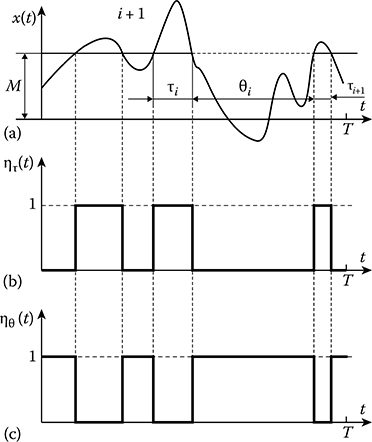
FIGURE 15.15 Transformation of stochastic process realization x(t) into the pulse sequence: (a) Example of stochastic process spike; (b) Pulse sequence normalized by the amplitude η_τ with duration T_i; (c) Pulse sequence normalized by the amplitude η_θ with duration θ_i.

15.6.1 Estimation of Spike Mean

Taking into consideration the assumptions stated previously, the estimate of the spike number in the given stochastic process realization x(t) within the limits of the observation time interval [0, T] at the level M can be defined approximately as

$N^{*} = \frac{1}{τ_{a v}} {\int^{}}_{T}^{0} η_{τ} (t) d t = \frac{1}{θ_{a v}} {\int^{}}_{0}^{T} η_{θ} (t) d t, (15.284)$

where τ_av and θ_av are the average duration of spike and the average interval between spikes within the limits of the observation time interval [0, T] of the given stochastic process realization at the level M. The true values of the average duration of spikes $\bar{τ}$ and the average interval between spikes $\bar{θ}$ obtained as a result of averaging by a set of realizations are defined in accordance with Ref. [1] in the following form:

$\bar{τ} = \frac{1}{\bar{N}} {\int^{}}_{M}^{\infty} p (x) d x = \frac{1}{\bar{N}} [1 - F (M)], (15.285)$

$\bar{θ} = \frac{1}{\bar{N}} \int_{- \infty}^{M} p (x) d x = \frac{F (M)}{\bar{N}}, (15.286)$

where

F(M) is the probability distribution function
$\bar{N}$ is the average number of spikes per unit time at the level M defined as

$\bar{N} = \int_{0}^{\infty} \dot{x} p_{2} (M, \dot{x}) d \dot{x}, (15.287)$

where p₂(M, ẋ) is the two-dimensional pdf of the stochastic process and its derivative at the same instant.

Note that $\bar{τ} = \bar{θ}$ corresponds to the level M₀ defined from the equality

$F (M_{0}) = 1 - F (M_{0}) = 0.5. (15.288)$

If the condition M ≫ M₀ is satisfied, the probability of event that on average there will be noninteger number of intervals between the stochastic process spikes θ_i within the limits of the observation time interval [0, T] high; otherwise, if the condition M ≪ M₀ is satisfied, the probability of event that on average there will be the noninteger number of spike duration τ_i within the limits of the observation time interval [0, T] is high. This phenomenon leads, on average, to more errors while measuring N* using the only formula (15.284). Because of this, while determining the statistical characteristics of the estimate of the average number of spikes, the following relationship

$N^{*} = {\begin{matrix} \frac{1}{\bar{θ}} {\int^{}}_{0}^{T} η_{θ} (t) d t a t M \leq M_{0} (\bar{τ} \geq \bar{θ}), \\ \frac{1}{\bar{τ}} {\int^{}}_{0}^{T} η_{τ} (t) d t a t M \geq M_{0} (\bar{τ} \leq \bar{θ}) \end{matrix} (15.289)$

can be considered as the first approximation, where we assume that

$\frac{τ_{av} - \bar{τ}}{\bar{τ}} ≪ and \frac{θ_{av} - \bar{θ}}{\bar{θ}} ≪ 1.$

For this reason, we use the approximations $τ_{av} \approx \bar{τ}$ and $θ_{av} \approx \bar{θ}$ .

The mathematical expectation of the average number of stochastic process spikes can be deter-mined in the following form:

$〈 N^{*} 〉 = {\begin{matrix} \frac{1}{\bar{θ}} {\int^{}}_{0}^{T} 〈 η_{θ} (t) 〉 d t a t M \leq M_{0} (\bar{τ} \geq \bar{θ}), \\ \frac{1}{\bar{τ}} {\int^{}}_{0}^{T} 〈 η_{τ} (t) 〉 d t a t M \geq M_{0} (\bar{τ} \leq \bar{θ}) . \end{matrix} (15.290)$

According to (15.282), (15.283), (15.285), and (15.286), we obtain

$〈 η_{θ} (t) 〉 = \int_{- \infty}^{M} p (x) d x = \bar{θ} \times \bar{N}, (15.291)$

$〈 η_{τ} (t) 〉 = {\int^{}}_{\infty}^{M} p (x) d x = \bar{τ} \times \bar{N} (15.292)$

Substituting (15.291) and (15.292) into (15.290), we obtain

$〈 N^{*} 〉 = \bar{N} \times T . (15.293)$

In other words, the estimate of average number of the stochastic process spikes at the level M within the limits of the observation time interval [0, T] is unbiased as a first approximation.

The estimate variance of the average number of stochastic process spikes at the level M can be presented in the following form:

${N^{*}} = {\begin{matrix} \frac{1}{\bar{θ}} {\int^{}}_{0}^{T} {\int^{}}_{0}^{T} 〈 η_{θ} (t_{1}) η_{θ} (t_{2}) 〉 d t_{1} d t_{2} - {[\bar{N} T]}^{2}, M \leq M_{0}, \\ \frac{1}{\bar{τ}} {\int^{}}_{0}^{T} {\int^{}}_{0}^{T} 〈 η_{τ} (t_{1}) η_{τ} (t_{2}) 〉 d t_{1} d t_{2} - {[\bar{N} T]}^{2}, M \geq M_{0} . \end{matrix} (15.294)$

In the case of ergodic stochastic processes, the average values can be written in the following form:

$〈 η_{θ} (t_{1}) η_{θ} (t_{2}) 〉 = R_{θ} (t_{1} - t_{2}) (15.295)$

and

$〈 η_{τ} (t_{1}) η_{τ} (t_{2}) 〉 = R_{τ} (t_{1} - t_{2}) . (15.296)$

As we can see from (15.295) and (15.296), the average values are equal to the probabilities of nonexceeding and exceeding the level M by the stochastic process realization x(t) at the instants t₁ and t₂

$R_{θ} (t_{1} - t_{2}) = \int_{- \infty}^{M} \int_{- \infty}^{M} p_{2} (x_{1}, x_{2}; t_{1} - t_{2}) d x_{1} d x_{2}; (15.297)$

$R_{τ} (t_{1} - t_{2}) = {\int^{}}_{M}^{\infty} {\int^{}}_{M}^{\infty} p_{2} (x_{1}, x_{2}; t_{1} - t_{2}) d x_{1} d x_{2} . (15.298)$

Taking into consideration. (15.294). through. (15.298), introducing new variables. t = t₁ − t₂, and changing the order of integration, we can write

$\frac{V a r {N^{*}}}{{[\bar{N} T]}^{2}} = {\begin{matrix} \frac{2}{T {F (M)}^{2}} {\int^{}}_{0}^{T} (1 - \frac{τ}{T}) R_{θ} (t) d t - 1, M \leq M_{0}, \\ \frac{2}{T {1 - F (M)}^{2}} {\int^{}}_{0}^{T} (1 - \frac{τ}{T}) R_{τ} (t) d t - 1, M \geq M_{0}, \end{matrix} (15.299)$

where $Var {N *} / {[\bar{N} T]}^{2}$ is the normalized variance of the average number of stochastic process spikes or the relative variance of the average number of stochastic process spikes.

As applied to the Gaussian and Rayleigh stochastic processes, we can present the two-dimensional probability distribution functions in the form (14.50) and (14.71). In the case of Gaussian stochastic process with zero mathematical expectation, that is, F(M₀) = 1 − F(M₀) at M₀ = 0 Substituting (14.50) into (15.297) and (15.298), we obtain

$R_{θ} (t) = (1 - Q {[\frac{M}{σ}]}^{2}) + {\sum^{}}_{v = 1}^{\infty} {1 - Q^{(v)} {[\frac{M}{σ}]}^{2}} \frac{R^{v} (t)}{v!}, (15.300)$

$R_{τ} (t) = {Q [\frac{M}{σ}]}^{2} + {\sum^{}}^{}_{\infty}^{v = 1} {1 - Q^{(v)} [\frac{M}{σ}]}^{2} \frac{R^{v} (t)}{v!} . (15.301)$

In accordance with (15.299), we obtain

$\frac{V a r {N^{*}}}{{[\bar{N} T]}^{2}} = {\begin{array}{l} {1 - Q [\frac{M}{σ}]}^{- 2} {\sum^{}}_{v = 1}^{\infty} a_{v} c_{v}, \frac{M}{σ} \leq 0, \\ {Q [\frac{M}{σ}]}^{- 2} {\sum^{}}_{v = 1}^{\infty} a_{v} c_{v,} \frac{M}{σ} \leq 0, \end{array} (15.302)$

where a_v and c_v are defined analogously as in (14.56) and (14.58). In doing so, the values of the coefficients a_v are presented in Table 14.1 as a function of v and the normalized level z = Mσ⁻¹.

Since

$1 - Q [- \frac{M}{σ}] = Q [- \frac{M}{σ}], (15.303)$

we can see from (15.302) that the normalized variance of the average number of stochastic process spikes $Var {N *} / {[\bar{N} T]}^{2}$ is symmetrical with respect to the level M/σ = 0. Because of this, we can write

$\frac{V a r {N^{*}}}{{[\bar{N} T]}^{2}} = {Q [| \frac{M}{σ} |]}^{- 2} {\sum^{}}_{v = 1}^{\infty} a_{v} c_{v} . (15.304)$

As applied to the Gaussian stochastic process with the normalized correlation function

$ℜ (t) = \exp {- α^{2} t^{2}}, (15.305)$

we obtain

$c_{v} = \frac{\sqrt{π}}{p \sqrt{v}} {1 - Q (p \sqrt{v}) + \frac{1 - \exp {- v p}}{p \sqrt{v}}}, (15.306)$

where p = αT. If p ≫ 1

$c_{v} = \frac{\sqrt{π}}{p \sqrt{v}}, (15.307)$

The normalized squared deviation of the average number of stochastic process spikes $\sqrt{Var {N *}} / [\bar{N} T]$ as a function of the normalized level |z = Mσ⁻¹| for realizations of stochastic process with fixed duration, the parameter p = αT is shown in Figure 15.16. As we can see from

Images

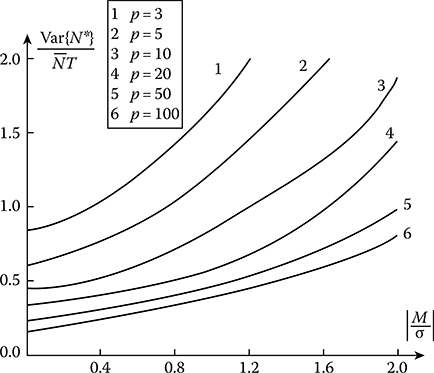
FIGURE 15.16 Normalized squared deviation of the average number of stochastic process spikes as a function of the normalized level for Gaussian realizations of a stochastic process with fixed duration.

Figure 15.16, the normalized squared deviation $\sqrt{Var {N *}} / [\bar{N} T]$ of the average number of stochastic process spikes is increased with increasing in the absolute level value |z = Mσ⁻¹| and decreasing the parameter p = αT. At p = αT ≥ 10 and |z = Mσ⁻¹| = 0, we can write

$\frac{V a r {N^{*}}}{{[\bar{N} T]}^{2}} \approx \frac{1.3}{α T} . (15.308)$

As applied to the Rayleigh stochastic process, we have that $\bar{τ} = 0$ when

$\frac{M}{\sqrt{2} σ} = \sqrt{\ln 2} \approx 0.83. (15.309)$

Substituting (14.71) into (15.297) and (15.298), we obtain

$R_{θ} (t) = [1 - \exp {- \frac{M^{2}}{2 σ^{2}}}]^{2} + {\sum^{}}_{v = 1}^{\infty} \frac{R^{2 v} (t)}{{(v!)}^{2}} \exp {- \frac{M^{2}}{σ^{2}}} {L_{v} [\frac{M^{2}}{2 σ^{2}}] - v L_{v - 1} [\frac{M^{2}}{2 σ^{2}}]}^{2}; (15.310)$

$R_{τ} (t) = \exp {- \frac{M^{2}}{2 σ^{2}}} + {\sum^{}}_{v = 1}^{\infty} \frac{R^{2 v} (t)}{{(v!)}^{2}} \exp {- \frac{M^{2}}{σ^{2}}} {L_{v} [\frac{M^{2}}{2 σ^{2}}] - v L_{v - 1} [\frac{M^{2}}{2 σ^{2}}]}^{2} . (15.311)$

In accordance with (15.299), we obtain

$\frac{V a r {N^{*}}}{{[\bar{N} T]}^{2}} = {\begin{array}{l} \exp {- \frac{M^{2}}{2 σ^{2}}} {\sum^{}}_{v = 1}^{\infty} b_{v} d_{v}, M \geq 0.83, \\ {1 - \exp {- \frac{M^{2}}{2 σ^{2}}}}^{- 2} {\sum^{}}_{v = 1}^{\infty} b_{v} d_{v}, M < 0.83, \end{array} (15.312)$

where b_v and d_v are defined analogously as in (14.86) and (14.83). The values of coefficients are given in Table 14.3. The normalized squared deviation of the average number of stochastic process spikes $\sqrt{Var {N *}} / [\bar{N} T]$ as a function of the normalized level $M / \sqrt{2 σ^{2}}$ at $p_{1} = \sqrt{2} α T = 10$ in the case of the exponential normalized correlation function given by (15.305) is shown in Figure 15.17. As we can see from Figure 15.17, the normalized squared deviation of the average number of stochastic process spikes $\sqrt{Var {N *}} / [\bar{N} T]$ increases with an increase in the deviation of the normalized level $M / \sqrt{2 σ^{2}}$ with respect to the median of the probability distribution function $M_{0} / \sqrt{2 σ^{2}} = \sqrt{\ln 2}$ at the fixed $p_{1} = \sqrt{2} α T$ . This phenomenon is explained by a decrease in the number of spikes higher or lower than the level $M_{0} / \sqrt{2 σ^{2}} = \sqrt{\ln 2}$ .

15.6.2 Estimation of Average Spike Duration and Average Interval Between Spikes

Considering the stochastic process realization presented in Figure 15.15a, we can see that with higher number of spikes N within the limits of the observation time interval [0, T] the estimate of spike duration average τ* and the estimate of average of the interval θ* between the spikes can be presented as

Images

FIGURE 15.17 Normalized squared deviation of the average number of stochastic process spikes as a function of the normalized level for Rayleigh realizations of the stochastic process with fixed duration.

${_{θ^{*} = \frac{1}{N} {\sum^{}}_{i = 1}^{N} θ_{i}'}^{τ^{*} = \frac{1}{N} {\sum_{i = 1}^{N} τ_{i}}^{}} (15.313)$

for the given realization. The relationships given by (15.313) can be presented in the following form:

${\begin{matrix} τ^{*} = \frac{1}{N} {\int^{}}_{0}^{T} η_{τ} (t) d t, \\ θ^{*} = \frac{1}{N} {\int^{}}_{0}^{T} η_{θ} (t) d t, \end{matrix} (15.314)$

where η_τ(t) and η_θ(t) are given by (15.282) and (15.283).

Images

FIGURE 15.18 Measurement of spike duration and the average of interval between the spikes.

The device to measure the spike duration average τ* and the average of interval θ* between the spikes can be designed based on (15.313) and (15.314). As applied to the estimate of the spike duration average τ*, the flowchart of measurer is depicted in Figure 15.18. This measurer consists of the trigger forming at the output normalized by amplitude and shape function η_τ(t), the counter of spikes, the integrator, and the divisor determining the estimate of spike duration average τ*. The threshold M is given by external source.

To define the statistical characteristics of estimates τ* and θ* we assume that the condition T ≫ τ_cor is satisfied. In this case, we can approximately assume $N \approx \bar{N} T$ Then

${\begin{matrix} τ^{*} = \frac{1}{\bar{N} T} {\int^{}}_{0}^{T} η_{τ} (t) d t, \\ θ^{*} = \frac{1}{\bar{N} T} {\int^{}}_{0}^{T} η_{θ} (t) d t, \end{matrix} (15.315)$

The mathematical expectation of estimates can be presented in the following form:

${\begin{matrix} 〈 τ^{*} 〉 = \frac{1}{\bar{N} T} {\int^{}}_{0}^{T} 〈 η_{τ} (r) 〉 d t, \\ 〈 θ^{*} 〉 = \frac{1}{\bar{N} T} {\int^{}}_{0}^{T} 〈 η_{θ} (t) 〉 d t, \end{matrix} (15.316)$

Taking into consideration (15.291) and (15.292), we see that $〈 τ * 〉 = \bar{τ}$ and $〈 θ * 〉 = \bar{θ}$ . In other words, the estimates of the spike duration average x* and the average of interval 8* between the spikes are unbiased as a first approximation.

Determine the estimate variance of the average spike duration of stochastic process at level M:

$V a r {τ^{*}} = 〈 (τ^{*} - \bar{τ})^{2} 〉 = \frac{1}{{[\bar{N} T]}^{2}} {\int^{}}_{0}^{T} {\int^{}}_{0}^{T} 〈 η_{τ} (t_{1}) η_{τ} (t_{2}) 〉 d t_{l} d t_{2} - {\bar{τ}}^{2} . (15.317)$

The mathematical expectation

$〈 η_{τ} (r_{1}) η_{τ} (r_{2}) 〉 = ℜ e_{τ} (t_{1} - t_{2}) (15.318)$

is defined by (15.298). By analogy with (15.299), we can define the estimate variance of the average spike duration τ*

$V a r {τ^{*}} = \frac{1}{{\bar{N}}^{2}} \times \frac{2}{T} {\int^{}}_{0}^{T} (1 - \frac{τ}{T}) ℜ_{τ} (t) d t - {\bar{τ}}^{2} . (15.319)$

The estimate variance of the average of interval θ*.between the spikes can be presented in the following form:

$V a r {θ^{*}} = \frac{1}{{\bar{N}}^{2}} \times \frac{2}{T} {\int^{}}_{0}^{T} (1 - \frac{τ}{T}) ℜ_{θ} (t) d t - {\bar{θ}}^{2} . (15.320)$

As applied to the Gaussian stochastic process, if the condition T ≫ τ_cor is satisfied the normalized correlation functions ℛ_τ(t) and ℛ_θ(t) are given by (15.300) and (15.301) and the average number of stochastic process spikes at level M can be determined as

$\bar{N} [\frac{M}{σ}] = \frac{1}{2 π} \sqrt{- {\frac{d^{2} ℛ (t)}{d t^{2}} |}_{t = 0}} \exp {- \frac{M^{2}}{2 σ^{2}}} . (15.321)$

Taking into consideration (15.285) and substituting (15.319), we obtain

$Var {τ^{*}} = \frac{8 π^{2}}{{T (d^{2} ℛ (t) / d t^{2}) |}_{t = 0}} \exp {\frac{M^{2}}{σ^{2}}} {\sum^{}}_{v = 1}^{\infty} α_{v} {\int^{}}_{0}^{T} ℛ^{v} (t) d t, (15.322)$

where α_v is given by (14.56) and Table 14.1. The formula (15.322) is correct for measuring the estimate variance of the average of interval θ* between the spikes.

As applied to the normalized correlation function given by (15.305), the estimate variance of the average spike duration τ*

$Var {τ^{*}} = \frac{2 π^{2} \sqrt{π}}{p} \exp {\frac{M^{2}}{σ^{2}}} {\sum^{}}_{v = 1}^{\infty} \frac{α_{v}}{\sqrt{v}}, (15.323)$

where p = αT. As we can see from (15.323), in the Gaussian stochastic process and the fixed duration of the observation interval [0, T] case, the estimate variance of the spike duration average τ* and the estimate variance of the average of interval θ* between the spikes are minimum at M/σ = 0.

As applied to the Rayleigh stochastic process, if the condition T ≫ τ_cor is satisfied the normalized correlation functions ℛ_τ(t) and ℛ_θ(t) are given by (15.310) and (15.311) and the average number of stochastic process spikes at level M can be determined as

$\bar{N} [\frac{M}{σ}] = \frac{1}{\sqrt{2 π}} \sqrt{- {\frac{d^{2} ℛ (t)}{d t^{2}} |}_{t = 0}} \exp {\frac{M}{σ}} \exp {- \frac{M^{2}}{2 σ^{2}}} . (15.324)$

Substituting ℛ_τ(t) into (15.319) and taking into consideration (15.285) and (15.324), we obtain

$Var {τ^{*}} = \frac{2 π}{{T (d^{2} ℛ (t) / d t^{2}) |}_{t = 0}} \exp {\frac{M^{2}}{σ^{2}}} \frac{2 σ^{2}}{M^{2}} {\sum^{}}_{v = 1}^{\infty} ℛ_{v} {\int^{}}_{0}^{T} ℛ^{2 v} (t) d t . (15.325)$

It is easy to prove that (15.235) is true to define the estimate variance of the average of interval θ*. between the spikes.

15.7 Mean-Square Frequency Estimate of Spectral Density

The mean-square frequency $\bar{f}$ given by (15.6) is widely used as a parameter characterizing the spectral density of stochastic process. The value $\bar{f}$ defines a dispersion of component of the stochastic process spectral density relative to zero frequency. As applied to low-frequency stationary stochastic processes, the mean-square frequency $\bar{f}$ characterizes the effective bandwidth of spectral density. Taking into consideration (15.259), we can present the mean-square frequency $\bar{f}$ in the following form:

$\bar{f} = \frac{1}{2 π} \sqrt{- {\frac{\frac{d^{2} R (τ)}{d τ^{2}}}{R (τ)} |}_{τ = 0} = \frac{1}{2 π} \sqrt{\frac{〈 {[\frac{d x (t)}{d t}]}^{2} 〉}{〈 x^{2} (t) 〉}} .} (15.326)$

Here and further, we assume that the investigated stochastic process possesses zero mathematical expectation. As applied to the Gaussian stochastic process, the mean-square frequency $\bar{f}$ is matched with the average number of stochastic process spikes per unit time at the zero level (15.321).

According to (15.326), it is worthwhile to consider for the investigated stationary stochastic process the following value

$\bar{f} = \frac{1}{2 π} \sqrt{\frac{\frac{1}{T} \int_{0}^{T} {[\frac{d x (t)}{d t}]}^{2} d t}{\frac{1}{T} \int_{0}^{T} x^{2} (t) d t}} (15.327)$

as the estimate of the mean-square frequency that tends to approach $\bar{f}$ as T → ∞. The flowchart of measurer of the mean-square frequency of the stochastic process is shown in Figure 15.19. To define the characteristics of the mean-square frequency estimate we can use the following representation of numerator and denominator in (15.327) in the following form:

$\frac{1}{T} {\int^{}}_{0}^{T} {[\frac{d x (t)}{d t}]}^{2} d t = {Var}_{\dot{x}} + Δ {Var}_{\dot{x}}, (15.328)$

$\frac{1}{T} {\int^{}}_{0}^{T} x^{2} (t) d t = {Var}_{x} + Δ {Var}_{x}, (15.329)$

where

Var_x and ${Var}_{\dot{x}}$ are the mathematical expectations of variances of the stochastic process and its derivative
ΔVar_x and Δ ${Var}_{\dot{x}}$ are the random errors of defnition of the earliermentioned variances within the limits of the finite observation time interval [0, T]

Images

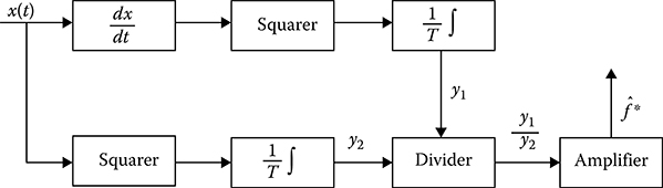
FIGURE 15.19 Measurement of the averaged squared frequency of stochastic process.

As we discussed before, the estimates of variances are unbiased and the variances of variance estimates are defined by (13.62) where we need to use the corresponding correlation function of the investigated stochastic process and its first derivative instead σ²ℛ(τ).

Going forward, we assume that the condition T ≫ τ_cor is satisfied. In this case, the errors ΔVar_x, and Δ ${Var}_{\dot{x}}$ will be small compared to Var_x and ${Var}_{\dot{x}}$ . To define the bias of the mean-square frequency under previous assumptions, we can think that

${\bar{f}}^{*} = \frac{1}{2 π} \sqrt{\frac{{Var}_{\dot{x}} + Δ {Var}_{\dot{x}}}{{Var}_{x} + Δ {Var}_{x}}} = \bar{f} \sqrt{\frac{1 + \frac{Δ {Var}_{\dot{x}}}{{Var}_{\dot{x}}}}{1 + \frac{Δ {Var}_{x}}{{Var}_{x}}} \approx} \bar{f} {1 + \frac{1}{2} \frac{Δ {Var}_{x}}{{Var}_{x}} - \frac{1}{8} \frac{Δ {Var}_{\dot{x}}^{2}}{{Var}_{\dot{x}}^{2}}} {11 \frac{1}{2} \frac{Δ {Var}_{x}}{{Var}_{x}} + \frac{3}{8} \frac{Δ {Var}_{x}^{2}}{{Var}_{x}^{2}}} . (15.330)$

Now, we are able to obtain the relative bias of estimate

$\frac{〈 Δ \bar{f} 〉}{\bar{f}} = \frac{〈 {\bar{f}}^{*} - \bar{f} 〉}{\bar{f}} \approx - \frac{1}{8} {\frac{〈 Δ {Var}_{\dot{x}}^{2} 〉}{V a r_{x}^{2}} - 3 \frac{〈 Δ {Var}_{x}^{2} 〉}{{Var}_{x}^{2}} + 2 \frac{〈 Δ {Var}_{x} Δ {Var}_{x} 〉}{{Var}_{x} {Var}_{x}}}, (15.331)$

where under the condition T ≫ τ_cor we have

$〈 Δ {Var}_{\dot{x}} Δ {Var}_{x} 〉 = \frac{4}{T} {\int^{}}_{0}^{T} {\frac{d R (τ)}{d τ}}^{2} d τ . (15.332)$

As a result, the relative bias can be presented in the following form:

$\frac{〈 Δ \bar{f} 〉}{\bar{f}} = \frac{1}{2 T} {- {\int^{}}_{0}^{\infty} {[\frac{ℛ 〞 (τ)}{ℛ 〞 (0)}]}^{2} d τ + 3 {\int^{}}_{0}^{\infty} ℛ^{2} (τ) d τ + 2 {\int^{}}_{0}^{\infty} \frac{ℛ^{' 2} (τ)}{ℛ 〞 (0)} d τ}, (15.333)$

where ℛ(τ), ℛ′(τ), and ℛ″(τ) are the normalized correlation function of the investigated stochastic process and its first and second derivatives. As applied to the exponential normalized correlation function of the investigated stochastic process given by (15.305), we can write

$\frac{〈 Δ \bar{f} 〉}{\bar{f}} = \frac{5 \sqrt{2 π}}{32 α T}, (15.334)$

that is, it means that the bias of estimate is inversely proportional to the observation time interval T.

Define a dispersion of the mean-square frequency estimate

$D {{\bar{f}}^{*}} = 〈 {({\bar{f}}^{*} - \bar{f})}^{2} 〉 = {\bar{f}}^{2} 〈 {\frac{1 + \frac{Δ {Var}_{\dot{x}}^{2}}{{Var}_{\dot{x}}}}{1 + \frac{Δ {Var}_{x}}{{Var}_{x}}} + 1 - 2 \frac{1 + \frac{Δ {Var}_{\dot{x}}}{{Var}_{\dot{x}}}}{1 + \frac{Δ {Var}_{x}}{{Var}_{x}}}} 〉 . (15.335)$

Using two-dimensional Taylor expansion in series for the first and third terms in (15.335) about the points

$\begin{matrix} \frac{Δ {Var}_{\dot{x}}}{{Var}_{\dot{x}}} = 0 & and & \frac{Δ {Var}_{x}}{{Var}_{x}} = 0 \end{matrix}$

and limiting by terms of the second order, we obtain

$\begin{array}{l} \frac{D {{\bar{f}}^{*}}}{{\bar{f}}^{2}} \approx & 〈 {{1 + \frac{Δ {Var}_{\dot{x}}}{{Var}_{\dot{x}}}} {1 - \frac{Δ {Var}_{x}}{{Var}_{x}} + \frac{Δ {Var}_{x}^{2}}{{Var}_{x}^{2}}} + 1 - 2 {1 + \frac{1}{2} \frac{Δ {Var}_{\dot{x}}}{{Var}_{\dot{x}}} - \frac{1}{8} \frac{Δ {Var}_{\dot{x}}^{2}}{{Var}_{\dot{x}}^{2}}}} \\ \times {1 - \frac{1}{2} \frac{Δ {Var}_{x}}{{Var}_{x}} + \frac{3}{8} \frac{Δ {Var}_{x}^{2}}{{Var}_{x}^{2}}} 〉 . \end{array} (15.336)$

Under averaging to a first approximation, we obtain

$\frac{D {{\bar{f}}^{*}}}{{\bar{f}}^{2}} \approx \frac{1}{T} {{\int^{}}_{0}^{\infty} {[\frac{ℛ 〞 (τ)}{ℛ 〞 (0)}]}^{2} d τ + {\int^{}}_{0}^{\infty} ℛ^{2} (τ) d τ + 2 {\int^{}}_{0}^{\infty} \frac{ℛ^{' 2} (τ)}{ℛ 〞 (0)} d τ} . (15.337)$

As applied to the exponential normalized correlation function given by (15.305), we obtain

$\frac{D {{\bar{f}}^{*}}}{{\bar{f}}^{2}} \approx \frac{3 \sqrt{2 π}}{16 α T} \approx \frac{0.47}{α T} . (15.338)$

Comparing (15.338) with the relative variance of estimate of the average number of Gaussian stochastic process spikes for the same normalized correlation function given by (15.308), we see that according to (15.326), the average mean-square frequency estimate or the average number of spikes leads to the bias of estimate and decrease in estimate dispersion approximately in 2.8 times.

15.8 Summary and Discussion

Methods of the correlation function estimate can be classifed on three groups subject to a principle of realization of delay and other elements of correlators: analog, digital, and analog-to-digital. In turn, the analog measurement procedures can be divided based on the methods using a representation of the investigated stochastic process both as the continuous process and as the sampled process. As a rule, physical delays are used by analog methods with continuous representation of the investigated stochastic process. Under discretization of investigated stochastic process in time, the physical delay line can be changed by corresponding circuits. Under the use of digital procedures to measure the correlation function estimate, the stochastic process is sampled in time and transformed into binary number by analog-to-digital conversion. Further operations associated with the signal delay, multiplication, and integration are carried out by the shift registers, summator, and so on.

We can see that the maximum value of variance of the correlation function estimate corresponds to the case τ = 0 and is equal to the variance of the stochastic process variance estimate given by (13.61) and (13.62). Minimum value of variance of the correlation function estimate corresponds to the case when τ ≫ τ_cor and is equal to one-half of the variance of the stochastic process variance estimate.

The correlation function of stationary stochastic process can be presented in the form of expansion in series with respect to earlier-given normalized orthogonal functions. The variance of correlation function estimate increases with an increase in the number of terms of expansion in series v. Because of this, we must take into consideration this fact choosing the number of terms under expansion in series.

In some practical problems, the correlation function of stochastic process can be measured accurately with some parameters defning a character of its behavior. In this case, the measurement of correlation function can be reduced to measurement or estimation of unknown parameters of correlation function. Because of this, we consider the optimal estimate of correlation function arbitrary parameter assuming that the investigated stochastic process ξ(t) is the stationary Gaussian stochastic process observed within the limits of time interval [0, T] in the background of Gaussian stationary noise ζ(t) with known correlation function.

The optimal estimate of stochastic process correlation function can be found in the form of estimations of the elements R_ij of the correlation matrix R or elements C_ij of the inverse matrix C. In the case of Gaussian stationary stochastic process with the multidimensional pdf given by (12.169), the solution of likelihood ratio equation allows us to obtain the estimates C_ij and, consequently, the estimates of elements R_ij of the correlation matrix R.

Based on (15.272), we can design the flowchart of spectral density measurer shown in Figure 15.13. The spectral density value at the fixed frequency coincides accurately within the constant factor with the variance of stochastic process at the filter output with known bandwidth. Operation principles of the spectral density measurer are evident from Figure 15.13. To define the spectral density for all possible values of frequencies, we need to design the multichannel spectrum analyzer and the central frequency of narrowband filter must be changed discretely or continuously. As a rule, we need to carry out a shift by the spectrum frequency of the investigated stochastic process using, for example, the linear law of frequency transformation instead of filter tuning by frequency. The structure of such measurer is depicted in Figure 15.14. The sawtooth generator controls the operation of measurer changing a frequency of heterodyne.

In many applications, we need to know the statistical parameters of stochastic process spike (see Figure 15.15a): the spike mean or the average number of down-up cross sections of some horizontal level M within the limits of the observation time interval [0, T], the average duration of spike, and the average interval between spikes. To measure these parameters of spikes, the stochastic process realization x(t) is transformed by the nonlinear transformer (threshold circuitry) into the pulse sequence normalized by the amplitude η_τ with duration τ_i (Figure 15.15b) or normalized by the amplitude η_θ with duration θ_i (Figure 15.15c).

The mean-square frequency $\bar{f}$ given by (15.6) is widely used as a parameter characterizing the spectral density of the stochastic process. The value $\bar{f}$ defines a dispersion of component of the stochastic process spectral density relative to zero frequency. As applied to low-frequency stationary stochastic processes, the mean-square frequency $\bar{f}$ characterizes the effective bandwidth of spectral density.

References

1. Lunge, F. 1963. Correlation Electronics. Leningrad, Russia: Nauka.

2. Ball, G.A. 1968. Instrumental Correlation Analysis of Stochastic Processes. Moscow, Russia: Energy.

3. Kay, S.M. 1993. Fundamentals of Statistical Signal Processing: Estimation Theory. Upper Saddle River, NJ: Prentice Hall, Inc.

4. Lampard, D.G. 1955. New method of determining correlation functions of stationary time series. Proceedings of the IEE, C-102(1): 343.

5. Kay, S.M. 1998. Fundamentals of Statistical Signal Processing: Detection Theory. Upper Saddle River, NJ: Prentice Hall, Inc.

6. Gribanov, Yu I. and V.L. Malkov. 1978. Selected Estimates of Spectral Characteristics of Stationary Stochastic Processes. Moscow, Russia: Energy.

..................Content has been hidden....................

You can't read the all page of ebook, please click here login for view all page.

Table of Contents for
Chapter 15 Estimate of Stochastic Process Frequency-Time Parameters

15 Estimate of Stochastic Process Frequency-Time Parameters

15.1 Estimate of Correlation Function

15.2 Correlation Function Estimation Based on its Expansion in Series

15.3 Optimal Estimation of Gaussian Stochastic Process Correlation Function Parameter

15.4 Correlation Function Estimation Methods Based on other Principles

15.5 Spectral Density Estimate Of Stationary Stochastic Process

15.6 Estimate of Stochastic Process Spike Parameters

15.6.1 Estimation of Spike Mean

15.6.2 Estimation of Average Spike Duration and Average Interval Between Spikes

15.7 Mean-Square Frequency Estimate of Spectral Density

15.8 Summary and Discussion

References

Table of Contents for Chapter 15 Estimate of Stochastic Process Frequency-Time Parameters

Create new playlist

Sign In

Sign Up

Table of Contents for
Chapter 15 Estimate of Stochastic Process Frequency-Time Parameters