
6 Principles of Control Algorithm Design for Complex Radar System Functioning at Dynamical Mode
An elementary basic flowchart presenting the subsystems usually found in a radar is shown in Figure 6.1. The transmitter, which is shown here as a power amplifier, generates a suitable waveform for the particular job the radar is to perform. It might have an average power as small as milliwatts or as large as megawatts. The average power is a far better indication of the capability of a radar’s performance than its peak power. Most radars use a short-pulse waveform so that a single antenna can be used on a time-shared basis for both transmitting and receiving. The function of the duplexer is to allow a single antenna to be used by protecting the sensitive receiver from burning out while the transmitter is on and by directing the received echo signal to the receiver rather than to the transmitter. The antenna is the device that allows the transmitted energy to be propagated into space and then collects the echo energy on receiver. It is almost always a directive antenna, one that directs the radiated energy into a narrow beam to concentrate the power as well as to allow the determination of the direction of the target. An antenna that produces a narrow directive beam on transmit usually has a large area on receive to allow the collection of weak echo signals from target. The antenna not only concentrates the energy on transmit and collects the echo energy on receive but it also acts as a spatial filter to provide angle resolution and other capabilities.
The receiver amplifies the weak received signal to a level where its presence can be detected. Because noise is the ultimate limitation on the ability of a radar to make a reliable detection decision and extract information about the target, care is taken to ensure that the receiver produces very little noise of its own. At the microwave frequencies, where most radars are found, the noise that affects radar performance is usually from the first stage of the receiver, shown here in Figure 6.1 as a low-noise amplifier. For many radar applications where the limitation to detection is the unwanted radar echoes from the environment called the clutter, the receiver needs to have a large enough dynamic range so as to avoid having the clutter echoes adversely affect detection of wanted moving targets by causing the receiver to saturate. The dynamic range of the receiver, usually expressed in decibels, is defined as the ratio of the maximum to the minimum signal input power levels over which the receiver can operate with some specified performance. The maximum signal level might be set by the nonlinear effects of the receiver response that can be tolerated, for example, the signal power at which the receiver begins to saturate, and the minimum signal might be the minimum detectable signal. The signal processor, which is often in the intermediate frequency portion of the receiver, might be described as being the part of the receiver that separates the desired signal from the undesired signals that can degrade the detection process. Signal processing includes the generalized detector that maximizes the output signal-to-noise ratio (SNR). Signal processing also includes the Doppler processing that maximizes the signal-to-clutter ratio of a moving target when clutter is larger than the receiver noise, and it separates one moving target from other moving targets or from clutter echoes. The detection decision is made at the output of the receiver, so a target is declared to be present when the receiver output exceeds a predetermined threshold. If the threshold is set too low, the receiver noise can cause excessive false alarms. If the threshold is set too high, detections of some targets might be missed that would otherwise have been detected. The criterion to determine the level of the decision threshold is to set the threshold so that it produces an acceptable predetermined average rate of false alarms due to receiver noise.
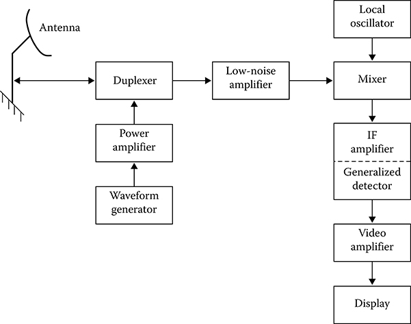
FIGURE 6.1 Flowchart of radar system.
After the detection decision is made, the track of a target can be determined, where a track is the locus of target locations measured over time. This is an example of data processing. The processed target detection information or its track might be displayed to an operator; or the detection information might be used to automatically direct a missile to a target; or the radar output might be further processed to provide other information about the nature of the target. The radar control ensures that the various parts of radar operate in a coordinated and cooperative manner, as, for example, providing timing signals to various parts of the radar as required.
The radar engineer has a resource time that allows good Doppler processing, bandwidth for good range resolution, space that allows a large antenna, and energy for long-range performance and accurate measurements. External factors affecting radar performance include the target characteristics; external noise that might enter via the antenna; unwanted clutter echoes from land, sea, birds, or rain; interference from other electromagnetic radiators; and propagation effects due to the Earth’s surface and atmosphere. These factors are mentioned here to emphasize that they can be highly important in the design and application of radar systems.
6.1 Configuration and Flowchart of Radar Control Subsystem
The radar control subsystem is considered as a purposeful change in the structure of a complex radar system (CRS) and, as a consequence, a variation of radar subsystem parameters to reach a maximum effect under radar control. The main tasks of a complex radar control subsystem are to organize an optimal functioning of the radar system as a subsystem in the control subsystem of a higher level. A necessity to control the parameters and structure of a CRS in dynamical mode is caused by the complexity and abruptness of environment conditions, that is, man-made and/ or echo interferences, reflection from the Earth’s surface, various objects, such as trees, buildings, hydrometeors, and so on, transient observations, a variety of problems that are to be solved, and limitations in energy and computational resources of the CRS. Hence, the control subsystem must be considered, first, as the means toward this end assigned for the CRS and, second, as a method to compensate for unwanted changes in environment that are interferences for its optimal functioning [1].
The main requirement to organize the control subsystem in a CRS structure is the knowledge of controlled parameters. If the number of controlled parameters is increased, the possibilities to organize the control system become high. Most control problems can be solved by multifunctional complex radar subsystems [2–7]. Therefore, in this chapter we consider mainly the problem statements and solutions of control problems in CRSs of this kind. Henceforth, all necessary signal and data processing algorithms assigned to reach the given control goal are considered as the control subsystem of a CRS. In doing so, the word control is used to designate both a process to reach the assigned task and in the sense of purposeful impact on parameters and structure of complex radar subsystems.
The first stage of designing the CRS control subsystem is a choice or formalization of goals, which must be attained in the course of controlling. In a general case, a high-level efficacy of CRS functioning is the main aim of a control subsystem. A degree of fulfillment of this aim can be evaluated by estimation of the vector Y(t)—the output parameters of a CRS—that is used to define its efficacy index: W = W[Y(t)] [8–10]. To realize the control subsystem, there is a need to design control subsystem channels to transfer control signal U(t). Internal parameters and methods of limited resource consumption of CRS are the object of a control subsystem. The figure of merit of required information is a function of an environment statement Z(t), the set of the internal parameters XU(t) corrected by the control system, and special controlling decision U(t):
where F is the vector-operator of the controlled object functioning. In a general case, the goal of a control subsystem is to obtain such values of the vector Y(t) = Y• (t) that ensure a condition
Now, informed about the environment conditions, controlled object, and control subsystem aim, we are able to present the control signal U(t) in the form of an algorithm:
Owing to the complexity of a radar system as a controlled object, the solution of the control problem, in a general form, has some difficulties. On the one hand, these difficulties are caused by the required computer costs and RAM size to solve the control problems within the limits of very short and strictly limited time intervals defined by dynamical changes of environment and CRS functioning. On the other hand, these difficulties have a principal character, since there are no methods of formalization and optimization of the control problem, which allow us to obtain a quantitative assessment as a whole for such a system as the CRS. Hence, in the course of designing the CRS control subsystem, the well-known system engineering procedure of complex system division in individual subsystems is widely used. In doing so, a choice of the structure and dimension of subsystem is carried out in accordance with universally adopted principles to save the backbone connections, and also taking into consideration the definite stages of CRS signal processing. Naturally, in division we should take into consideration possibilities to ensure the best control process for subsystems and the CRS as a whole. Division or decomposition of the CRS into subsystems assumes that each subsystem has a criterion function to control that is generated from a general objective function of the CRS.
To increase efficiency and decrease work content for the solution of control tasks, a subsystem of control algorithms is designed based on a hierarchical approach [11]. The hierarchical structure of the control subsystem is characterized by the presence of some control levels associated with each other, by which a general task is divided. In doing so, the control algorithms of high levels define and coordinate the working abilities of lower levels. Based on the aforementioned general statements, the CRS, as an object to control, can be divided into controlled subsystems, including the signal detection and signal processing subsystems. The controlled subsystems are as follows:
Transmit and receive antenna with controlled parameters:
The number of generated beams of transmit Ntr and receive Nr antennas
The directional diagram beam width of the transmit
(θtrβ,θtrε) and receive(θrβ,θrε) antennasA degree of beam overlapping for the multibeam receive antenna directional diagram (δβr, δεr)
Function of changes in the main lobe direction of the transmit antenna directional diagram (β0, ε0)
The number and direction of radar antenna directional diagram valleys
Transmitter with controlled parameters:
The duration of searching signal τs
The power of transmitted pulse Pp
The carrier frequency fc or sequence of carrier frequencies {fci} under multifrequency operation
The spectrum bandwidth of searching signals Δfs
The parameters and way of chirp modulation of searching signals
The frequency F of searching signal repetition
Receiver with controlled parameters:
The optimal structure with a viewpoint of the maximal SNR under conditions of complex noise environment
Operation mode
The spectrum bandwidth of input linear tract Δfr
The dimension of gated area—the number of elements in the gate and coordinates of the gate center
Signal preprocessing processor of target return signals with controlled parameters:
The number of signal processing stages under detection and estimation of target return signal parameters
The upper A and lower B detection thresholds under sequential detection of target return signals
The truncation threshold ntr under sequential analysis of target return signals
The number N of accumulated pulses by detector with the fixed sample number
The threshold U0 of binary quantization
The logic operations (l, m, k) under detection of binary quantized target return signals
Signal reprocessing processor of target return signals and preparation of obtained information for user with controlled parameters:
The criterion to begin the target track (“2/m + l/n”)
The criterion to cancel the target range tracking
kcantr The algorithm and parameters of the linear filter used under the target range tracking
The way of refreshment of the tracked target
The target range parameters and precision characteristics transmitted to the user
The majority of controlled parameters of the CRS and signal processing subsystems depend on each other. For instance, the duration of the scanning signal τs, the period or frequency of repetition T or F, the power of transmitted pulse Pp, and the average power of scanning signal
As the average power of scanning signal
The radar antenna directional diagram beam width depends on the angle between the main axis of radar antenna and antenna beam:
where θ0 is the beam width in the main axis direction of the radar antenna. The radar antenna directional diagram beam broadening under misalignment of radar antenna leads us to a decrease in the coefficient of amplification of radar antenna, and consequently, to increasing the required number N of accumulated target return signals to ensure the given SNR by power. There are other associations that must be taken into consideration under the control process. Interrelating control parameters do not allow us to organize a control process insulatedly by each of the controlled blocks or subsystems of the CRS, which indicates the impossibility of spatial division of the control subsystem. At the same time, a specificity of the CRS operation allows us to organize a control process step by step in time and design a multilevel hierarchical structure of the control subsystem (see Figure 6.2).
The first level is the control of CRS and signal processing subsystem parameters and in the course of searching for the preliminary chosen direction in radar coverage taking into consideration a radar functional operation, namely, searching, target range tracking, and so on. Objective control function at this stage is to ensure a minimal energy consumption to obtain the given effect from searching the chosen direction, namely, the given probability of detection PD, the given accuracy to measure angle coordinates
The second control level is an optimization of CRS functional modes. In the case of radar target detection and target range tracking subsystems, there is a need to optimize a searching of new targets and target range tracking functioning. A way to observe the radar coverage and ability to refresh the tracked targets are the controlled functions. The objective function of an optimal control process is the minimization of specific CRS power resource consumption to detect the target under scanning, refreshment, and estimation of target range track parameters under target tracking. CRS technical parameters and specifications of the high-level system are the main limitations for target range tracking. The control process at the second level is carried out by optimal scheduling of radar coverage element observation in the scanning mode and refreshes each target during the target tracking mode. Periodicity of changes in the control process at this stage is mainly defined by dynamics of dirty data within the limits of radar coverage—the number of targets, importance of targets, environmental noise, and so on.

FIGURE 6.2 Hierarchical control system.
The third control level is a distribution of limited CRS power resources between functional modes: the detection and target tracking modes in the case of two functional CRSs. The objective functions of optimal control at this stage are the maximization of CRS efficiency criterion for higher hierarchical level, at which the CRS operates as the detection and target tracking system, and the maximization of the processed target number taking into consideration their importance. The control process at the third level is carried out by the redistribution of power resource parts assigned for scanning and target tracking modes. The periodicity of the control process depends on the a priori and a posteriori environment data within the radar range and ability of facilities for target servicing and so on.
The fourth control level is an administration to keep the CRS under required operational conditions taking into consideration information about the operation quality of its subsystems, changed environment, information from subsystems of the same levels, and control commands from subsystems of a higher hierarchical level. At this level, a contingency administration is mainly carried out.
Thus, we obtain the multilevel hierarchical structure of a radar control subsystem, the simplest flowchart of which is shown in Figure 6.2. The hierarchy of control process is characterized by a sequential release of information from complex radar subsystem of higher to lower level subsystems. At the same time, the results of particular problem solutions at lower levels are used as the basis to make decisions at the higher level. Thus, information about the energy consumption for scanning in each direction, the number of detected targets, and the energy consumption under target tracking mode comes to the second-level subsystem as a result of the first-level task solutions. The information about the number of tracked targets
6.2 Direct Control of Complex Radar Subsystem Parameters
6.2.1 INITIAL CONDITIONS
The control process in the course of scanning the selected direction is carried out by direct choice of controlled parameters of the CRS and signal preprocessing subsystem with the purpose of adapting to dynamical environmental conditions under the given operation mode. The main modes of CRS functioning are as follows:
Scan new targets in radar coverage.
Refresh met target tracks or search mode of detected targets.
Other possible functioning modes can be considered as particular cases of the aforementioned modes. Additionally, an extension of the mode numbers does not change control process principles. The external environment for a CRS is characterized by the presence of targets, noise, and different kinds of interferences such as the following:
The inadvertent interference—radio radiation of the world network, various radio engineering systems, mobile systems, and so on
The lumped interference—radiation, the spectrum of which is concentrated in the neighborhood of the central or resonant frequency and, with a spectral bandwidth that is larger in comparison to the spectral bandwidth of the signal at the radar receiver or detector input
The pulse interference—a sharp short-term increase in the spectral power density of the additive noise that occurs within the spectrum bandwidth limits of the signal
The deliberate interference—the interference generated specifically for the purpose to reduce the efficiency and noise immunity of the CRS
Henceforth, we assume that all information about target conditions in radar coverage is reconstructed by the a priori and a posteriori data in the course of CRS operation. The noise environment is evaluated by a special signal processing subsystem assigned to analyze changed conditions of the environment. We assume that analysis of additive noise parameters, namely, the type, power level, spectral power density, and so on, is carried out immediately before scanning the chosen direction. Processing and analysis of passive interferences and inclusion of protective equipment against this kind of interferences are carried out by control facilities of signal preprocessing subsystems during scanning the radar coverage.
There is a need to take into consideration that the tasks of choice and task-oriented changes of complex radar subsystem parameters must be solved within the limits of finite time intervals. This requirement is very strong. In the course of the control process, the pulsing rate defined by repetition frequency cannot be changed and must be constant. All processes of decision making should be finished between neighboring scanning. In line with this, the table methods to make a decision can be widely used based on results of noise environment analysis in the radar range.
6.2.2 CONTROL UNDER DIRECTIONAL SCAN IN MODE OF SEARCHED NEW TARGETS
In this case, the control process is carried out by two stages. At the first stage, the calculation and choice of scanning signal parameters are carried out. The scanning signals must correspond to the functional mode of searching targets and maximal radar range in the given direction. Additionally, the receiver performance and signal processing algorithms for signal preprocessing subsystems should be defined and computed. This stage is carried out before scanning pulsing in the given direction. Control of accumulated received signals up to making decisions about the target detection/no detection using all resolution elements in the radar range (the case of sequential analysis) or up to accumulation of a determined number of the target return signals using detectors with the fixed sample sizes is carried out at the second stage. In the course of accumulation of the target return signals, the initial parameter values of scanning signals are the same excepting the carrier frequency fc. In the following, we give a description of a logical algorithmic flowchart to solve the control tasks under direction scanning using the searching mode (see Figure 6.3).
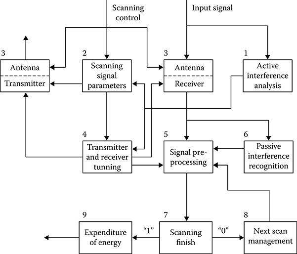
FIGURE 6.3 Logical structure of algorithm to search for a direction in the scanning mode.
Step 1: After setting transmit and receive antenna beams along the given direction βi, εi, we carry out an analysis of active interferences received along this direction (block 1). First of all, we should define the power
σ2n and the power spectral density N(f) of the noise. Evaluation of the noise power is used further to make a decision to power on that or other protection equipment from active interferences and, also, to determine predetection SNR. Estimation of power spectral density of active interferences allows us to define the “spectrum troubles” of interference within the limits of considered frequency bandwidth and select the scanning signal carrier frequency on the interval where an action of interference is weakest. In a general case, under analysis of interference there is a need to distinguish and classify the active interferences with definite integrity to create a possibility to use the obtained results to tune and learn the radar receiving channel.Step 2: At this stage, we solve the problems of the scanning signal parameter selection (block 2). For this purpose, first of all, there is a need to determine a distance
rεi from the radar to the radar coverage bound under the given elevation angle value εi. Computation is carried out taking into consideration the shape of radar antenna directional diagram. For scanning and tracking radar, a vertical cross section of idealized zone of target searching is shown in Figure 6.4. All searching zone characteristics are considered unknown.2.1 As it follows from the geometry presented in Figure 6.4, if εmax > εn > ε0, we have
rεi=REarth+Hmaxsin(0.5π+εi)sinγi,(6.6) 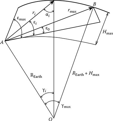
FIGURE 6.4 Vertical cross section of ideal target scanning zone.
where
γi=0.5π−εj−αjandγi<0.5π;(6.7) sinαi=REarthsin(0.5π+εi)REarth+Hmax,αi<0.5π.(6.8) Determination of
rεi can be made in advance for the whole range of the elevation angles ε0…εmax with discrete equal, for example, to the radar antenna directional diagram width in vertical plane.2.2 At the known range
rεi , the period of pulsing is determined from relationTi=2rεic,(6.9) where c = 3 × 10⁸ m/s.
2.3 The nonmodulated scanning signal with duration of τs is selected under the searching mode.
2.4 The pulse power of the scanning signal is given by
Ppi=P¯¯¯sTiτ−1si.(6.10) Computed and selected parameters of scanning signals, namely, fc,
Ppi , Ti,τsi are set in the transmitter (block 3, Figure 6.3).
Step 3: Results of scanning signal parameter computation and selection are used to define the minimal SNR on the radar coverage bound and signal preprocessing algorithm adjustments related to SNR.
3.1 The energy of target return signal
Etg=PpiσsiGtriGriλ2Stg(4π)3r4εiK,(6.11) where
Gtr is the amplifier coefficient of transmit antenna in the direction of εi, βi
Gr is the amplifier coefficient of receive antenna in the direction of εi, βi; in doing so, in the case of phased array, we have
{Gtri=Gtr0cosβ′icosε′i;Gri=Gr0cosβ′icosε′i,(6.12) where
{β′i=∣∣βi−βangle∣∣<0.5π;ε′i=|εi−εangle|<0.5π,(6.13) Gtr0 andGr0 are the amplifier coefficients of transmit and receive antennas on the phased array axis, respectivelyβangle and εangle are the angular direction of phased array axis
axis Stg is the effective reflecting surface of target that is considered as standard in the course of detection performance computation
K is the generalized loss factor
3.2 The total noise power spectral density at the CRS receiver input without taking into consideration the passive interferences is given by
NΣ=N¯¯¯activeinμ+N0,(6.14) where
Nactivein is the average power spectral density of active interferencesμ is the coefficient of active interference suppression by compensating and other protection facilities
N0=2kTBN,(6.15) where
k is the Boltzmann constant
T is the absolute temperature
BN is the receiver bandwidth
3.3 The SNR by power for the radar range
rεi is determined bySNR=2EsNΣ.(6.16)
Step 4: This SNR is used later to adjust a control of the CRS signal preprocessing subsystem detectors, that is, to define the required number of scans to reach the given probability of detection PD and the probability of false alarm PF for detectors with the fixed sample size or to define the weights of units and zeros under sequential analysis of binary quantized target return signals (block 4, Figure 6.3). There is a need to note that a realization of the a priori operations discussed earlier on selection of parameters for transmitter, receiver, and signal processing subsystems must be carried out within the limits of finite time intervals or the so-called free running of sweep time equal to
(T−τmaxd) . Because of this, we can employ the tables of parameters and settings corresponding to discrete values of noise characteristics, elevation angles, and other given parameters that are kept in a memory device instead of detailed computations.Step 5: After finishing the preliminary stage, we can start the process of directional scanning and accumulation of target return signals (block 5, Figure 6.3) taking into account the results of distinguishing the passive interferences and using the protection facilities against the passive interferences (block 6, Figure 6.3). At this stage, the control process is carried out by the signal preprocessing subsystem algorithms in accordance with the operations realized by blocks 7 and 8, Figure 6.3.
After finishing the accumulation stage and making a decision about the scanned direction, the results of decision making are issued and expenditure of energy and timetable are computed to observe the scanned direction (block 9, Figure 6.3). The radar antenna beam control is assigned for an algorithm of scanning management in the searching mode or mode controller. In conclusion, we note once more that the discussed logical flowchart is the way only to assign a control process under the searching new target mode. Naturally, there are possibly other ways, but a general idea to control, namely parametric matching of CRS subsystems and signal and data processing subsystems with environmental parameters and solved problems and tasks is the same.
6.2.3 CONTROL PROCESS UNDER REFRESHMENT OF TARGET IN TARGET TRACING MODE
Consider a possible way to design a control algorithm to detect and measure target coordinates in the course of target tracking using information that is discretely refreshed in the CRS with a controlled radar antenna beam. At the same time, we use the following assumptions:
Time instants of regular refreshment of target tracking are computed each time after clarification of target tracing parameters at the previous step. Time intervals between the previous and next measurements are determined based on the condition of nonrotating radar.
Owing to possible overlapping of location intervals of the tracked targets and under stimulus of more foreground modes, delays of instruction executions, for example, the target coordinate measure, are possible. Probability and delay time are high, a loading of the CRS is high, or the number of targets in the radar coverage is high. To exclude cancellations of target tracking owing to the delays mentioned earlier, the possibility to expand a searching zone of regular renewed target pip by the angle coordinates and radar range is provided. Expanding in the searching zone by angular coordinates is carried out by assigning some additional directions of scanning around an extrapolated direction taking into consideration the target track parameters, the so-called additional target searching. The number of directions of the additional target searching is not high—from 3 to 5. Expanding in the searching zone by the radar range is carried out by increasing the dimensions of gate Δrgate.
Expanding in the searching zone is carried out also if there are misses of the target pips on target tracing during one or several scanning jobs.
In accordance with the assumptions discussed earlier, the control algorithm to measure the target coordinates in the course of target tracking mode is mainly reduced to carrying out the following operations (see Figure 6.5):
Computation of delay
Δτsi to start a service of the selected target t0 in comparison with the prearranged service starttspi . This delay is compared with the allowable one computed based on the given probability of the target pip hit belonging to the given target tracing, into the gate limited by the radar antenna directional diagram beam width by the angle coordinates and bounds of the analyzed part of the radar range (blocks 1 and 2, Figure 6.5).If the delay
Δτsi is less than allowable and there is no feature of miss, that is, the probability of miss Pmiss is equal to zero in the course of the previous session of the target coordinate renewal, a computation of narrow gate by the radar range is carried out and a location in the computed or extrapolated direction is also carried out (the blocks 3, 4, and 7).If the delay
Δτsi is greater than allowable one or Pmiss = 1, there is a need to compute a wide gate by the radar range and angle coordinates of the additional target searching directions (blocks 5 and 6, Figure 6.5). After that, a target return signal location is provided, at the beginning, in the extrapolated direction, and after, if the target is not detected in the extrapolated direction, there is a need to provide a search in additional directions until the detection of target pip is fixed in the regular direction of the entire assigned additional target searching directions observed (blocks 14 and 16, Figure 6.5).After selection of regular target location direction, we carry out an analysis of noise environment in this direction. Henceforward, the parameters of scanning signals are calculated or selected, and tuning of the receiver is carried out (block 8, Figure 6.5), and the control process is assigned to the signal preprocessing subsystem algorithm in the target tracking mode (blocks 9 and 10, Figure 6.5).
The amount of directional scanning in the target tracking mode is defined based on a condition to obtain the given accuracy to measure the radar range and angle target coordinates. In a hard noise environment, this number can be peak clipped based on established balance of expenditure of energy for the target searching and target tracking modes.

FIGURE 6.5 Flowchart of control algorithm to measure the target coordinates.
If the target has been detected and the target coordinates have been measured with the given accuracy, then the corresponding target pip is produced to clarify the target tracing parameters. After that, the costs of refreshment about the detected target tracing are fixed and the control process is assigned to a mode administrator (blocks 11–13, Figure 6.5).
If after observation of the entire assigned additional target searching directions the target has not been detected, then the algorithm of target tracing end detection is powered on, which produces a decision to continue or to stop target tracking of the considered target tracing (block 15, Figure 6.5). Naturally, in this case, the expenditure of energy is also fixed.
Thus, the considered control algorithm operates interactively in a close way with the algorithms of the main operations of signal preprocessing and reprocessing subsystems within the limits of gate coordinating these algorithms into the unique signal processing subsystem in the individual CRS target tracking mode with the control beam of radar antenna directional diagram.
6.3 Scan Control in New Target Searching Mode
6.3.1 PROBLEM STATEMENT AND CRITERIA OF SEARCHING CONTROL OPTIMALITY
The problem to control the searching mode is related to a class of observation control tasks from mathematical statistics and is given in the following form. Let the pdf p(x|λ) of the observed random variable X be not given completely and possess some indefinite parameter ν that is selected by the statistician before a next observation of the random variable X. Thus, the following relation takes a place:
In this case, there is a need to choose the parameter ν of the pdf p(x |λ, ν) before observation of the random variable X. As a result, the experimentator controlling the observations affects the statistical features of observed random variables.
In radar, the control process is based on obtaining the radar coverage scanning, selection of angle direction and interval on radar range scanning, shape of radar antenna directional diagram, type of searching signal, and so on. In our case, the control process of scanning is reduced to controlling the radar antenna directional diagram position, the shape and angle dimensions of which are fixed under the condition of realization of the discussed algorithms. Under synthesis of observation control algorithms, it is natural to follow the principle of average risk minimization, that is, minimization of losses arising under the decision error. However, in this case, a choice of the corresponding function of losses is a difficult problem.
As an example, consider the following discussion on generation of the quadratic function of losses widely known from the theory of statistical decisions [12–14]. Let a set of {Ntg; θ1, θ2,…, θN} be a description of a true situation in the radar coverage, where Ntg is the number of targets and θ1j are the target parameters. Let v(t, θi) be the loss function formed by the target with the parameter θi. Then
If we are able to define the a posteriori pdfs p(θi, |X, V), where X is the vector of observed data and V is the control vector under searching, then the average risk can be defined in the following form:
In this case, a minimization of the average risk given by (6.17) must be carried out by selection of the control vector:
It is clear that a realization of such criteria is very difficult, especially within the limited time to scan the radar coverage zone.
The information criterion of efficacy reducing to maximization of average amount of information during scanning and observation of radar coverage was suggested in Refs. [15,16]. By this criterion, the control must be organized in such a way that an increment of information would be obtained at each step of observation. In a general case, a solution by both criteria is difficult. An approximate approach is based on a set of assumptions, of which the following are important:
The problem is solved for a single target or set of uncorrelated targets.
The observation space consists of cells, and we can scan a single cell only within the limits of observation step (the scanning period); in this case, a control process is the integer scalar value υ coinciding with the number of observed cells.
The υth cell random value X observed under scanning is a scalar and subjected to the pdf p0(x) in the case of target absent and the pdf p1(x) if the target is present; These pdfs are considered as known.
6.3.2 OPTIMAL SCANNING CONTROL UNDER DETECTION OF SINGLE TARGET
We start an analysis of optimal control methods to scan with the simplest case, namely, the detection of a single target within the limits of radar coverage consisting of N cells. Assume that there is a single target in the radar coverage or there are no targets. If there are no targets in the radar coverage, then the target can appear during the time τ within the ith cell (i = 1, 2,…, N) with the probability Pτ(i). If there is a single target within the limits of radar coverage, the probability of appearance of new targets is equal to zero. The target can be replaced by cells of scanning area with the probability of passing Pτ(i|j). Under a synthesis of control algorithm, we can consider the time (the number of cycles) from the beginning of scan to the instant of target detection as a figure of merit. The optimization process of the control algorithm is a minimization of this time.
The main result of synthesis shows us that the optimal control algorithm of radar coverage scanning is reduced to get the a posteriori probabilities Pt(i) of target presence in the cells (i = 1, 2,…, N) and to select the cell for next scanning (i = υ), within the limits of which the a posteriori probabilities Pt(i) of target presence are maximal, that is,
In the absence of the a priori data, the initial values of the probability P0(i) at t = 0 are chosen based on the condition that the probability of target presence in any radar coverage cell is the same. After regular scanning (e. g., the υth cell) at the time instant tN the a posteriori probabilities of target presence in cells are defined by the formulas:
In the case that the radar coverage cell has been just scanned (i = υ),
PtN(υ)=P∗tN(υ)p1(x)[1−P∗tN(υ)]p0(x)+P∗tN(υ)p1(x);(6.22) In the case of no scanned radar coverage cells (i ≠ υ),
PtN(υ)=P∗tN(υ)p0(x)[1−P∗tN(υ)]p0(x)+P∗tN(υ)p1(x);(6.23) where
P∗tN(υ) is the a posteriori probability of target presence in the υth cell determined at the instant tN.
Thus, after scanning the υth cell, the probabilities of target presence both in the scanned cell and in the unscanned cells are changed and, for example, an increase in the probability of target presence in a single cell leads us to a decrease in the probability of target presence in other cells.
The next scanning of the ith cell will be over the time interval τ. For this reason, under computation of the a posteriori probability of target presence
The considered control algorithm operates in such a way that at the end of scanning the antenna beam is directed to the cell with the maximal a posteriori probability of target presence and is not able to be switched to scan other cells. The scanning stop is carried out when the given a posteriori probability of target presence is reached (the threshold).
6.3.3 OPTIMAL SCANNING CONTROL UNDER DETECTION OF UNKNOWN NUMBER OF TARGETS
As a model of a radar coverage situation, we consider an uncorrelated set of targets that appear and move within the limits of the radar coverage (from cell to cell) independently of each other. The probability of a presence in each cell of more than one target is equal to zero, which corresponds to a model of rarefied flow. As earlier, the probability of target appearance in the ith cell during the time τ is equal to Pτ(i), and replacement of targets from cell to cell is described by the passing probability Pτ (i|j). A procedure of optimal scanning is to choose that cell at the next step for which the a posteriori probability of target presence is maximal. However, the following fact plays a very important role in this procedure: there are several targets within the limits of the radar coverage. By this reason, there is a need to ensure a mode of sequential addressing to the different cells including the cells with the minimal probability of target presence. In accordance with this fact, a sequence of control algorithm operations must be the following:
At the beginning of scan when the a posteriori probabilities of target presence in the cells are low, the υth cell with the maximal probability Pt (υ) = max Pt (i) is selected to scan.
If after regular scanning the probability Pt(υ) is continuously increased, the scanning of theυth cell is continued until this probability reaches the threshold value C1 chosen based on a permissible value of the probability of false alarm PF. After that, a decision about a target presence in the given cell is made and scanning of this cell is stopped.
Scanning locator is switched on one no scanned cell with the maximal probability Pt(i). In doing so, if after regular scanning the a posteriori probability of target presence in this cell is decreased, there is a need to select the cell with the maximal value of the probability Pt(i) and scan this cell.
Scanning the cell with the decreased a posteriori probability of target presence is continued until this probability is less than the threshold value C2 defined based on a permissible number of cycles required to scan the “empty” cells.
The cell with the detected target is included in a set of candidates to be scanned after (owing to target moving) the fact when the probability of target presence in this cell becomes less than the threshold C1.
Thus, the control algorithm ensures a sequential addressing to the cells, including the cells with the low a posteriori probability of target presence. The considered algorithm is optimal based on the viewpoint of minimization of the number of scanning cycles T from the beginning of scan to the instant of detection of all targets. In this case, the a posteriori probabilities of target presence are determined by the following formulas:
In theυth cell after regular scanning—the formula (6.22)
In other no scanning cells
PtN(i)=P∗tN(i),i≠υ.(6.25)
Determination of the a posteriori probability of target presence at the instant tN + τ of next cell scanning taking into consideration the movement and appearance of new targets is carried out based on the following formula:
These formulas take into consideration a peculiarity of situation model within the limits of radar coverage, in accordance with which the cells are independent and changes in the a posteriori probability of target presence in one cell do not change the a posteriori probability of target presence in other cells. The disadvantage of the considered approach in the synthesis of the optimal scanning control algorithm under detection of targets is the fact that there are no limitations on power resources required to scan the radar coverage. Therefore, it is worthwhile to search another approach to solve the problem of scanning optimization within the limits of the radar coverage.
The criterion maximizing the mean of number of the detected targets during the fixed time TS is useful in this sense. In the case when the scanning model of radar coverage is in the form of cells, we have
where
where
ES is the energy during the scanning
Ncell is the number of cells within the radar coverage
Pt(i) is the a priori probability of target presence in the ith cell
φi is the energy to scan the ith cell
PS(φi) is the probability of target detection in the ith cell under the condition that the energy φi has been required to do it
The criterion (6.27) allows us to find the optimal distribution of limited power resources by the cells but says nothing about the optimal sequence of scanning all the cells. Naturally, we consider a possibility to combine the criteria (6.21) and (6.27) with the purpose of obtaining the conditions to minimize the time to detect all targets under the limited power resources required to carry out the scanning within the limits of the radar coverage. In this case, the problem of optimal scanning control must be solved in two stages:
Solving the problem (6.27), there is a need to find the optimal distribution of power resources required to scan the radar coverage expressed, for example, by the number of scanning cycles of each radar coverage cell.
Using the criterion (6.21) and distribution of power resources by the cells, there is a need to define the optimal sequence of scanning of the radar coverage cells. At the same time, it is permissible to use the queuing theory, in particular, the optimal rule of application service in decreasing order of the ratio Pt(i)/Ni where Ni is the number of scans in the radar coverage along the ith direction.
A sequence of statements for designing the optimal control algorithm follows:
Let there be the a priori data about the probabilities
PtN(i)(i=1, 2, …, N) of target presence in each radar coverage cell at the time instant tN.Let the power resources to scan the radar coverage be given by the number N0 of scanning at the constant cycle T of searching signals.
If for each cell of radar coverage the maximal radar range
Rmaxi and the effective scattering areaStgi of target (the pulse power Pp and pulse duration τp are known) are given, we are able to define the energy of target return signalEsi under single scanning; the total power spectral density of the interference and noiseNΣi ; SNR under scanning by a single pulse (the radar receiver is constructed based on the generalized detector)SNRi=q2i=Esi/NΣi ; SNR under scanning by Ni signals is given bySNRNi=q2Ni=Niq2i .We assume, for example, that during scanning the ith cell, the target return signal is a noncoherent pulse train with independent fluctuation according to the Rayleigh in-phase and quadrature components. In this case, the conditional probability of false alarm PF and the probability of detection PD of the pulse train consisting of Ni pulses are determined by the following formulas [15]:
PF(Ni)=12Ni(Ni−1)!∫Kg∞XNi−1iexp(−0.5Xi)dXi;(6.29) PD(Ni)=12Ni(Ni−1)!∫Kg/(1+q2i)∞XNi−1iexp(−0.5Xi)dXi,(6.30) where
Xi is the sum of normalized voltage amplitudes (the signal + the noise) at the GD output
Kg is the normalized threshold used under detection of target return signals by GD determined based on required values of the probability of false alarm PF
The problem of optimal distribution of power resources by cells within the limits of the radar coverage for a single scanning is solved by assigning the number of pulses Ni with the purpose to scan each cell, that is,
E{N0}=maxNi∑i=1NtgPt(i)Ps(Ni),∑i=1NtgNi=N0.(6.31) As a result, we obtain a set of pulse trains of the signals
N1, N2,…,NNtg to scan all cells within the limits of the radar coverage.We define the ratios Pt(i)/Ni and arrange them in decreasing order. After that we start a sequential scanning of the cells using the serial numbers of ratios Pt (i)/Ni.
Thus, we have a principal possibility to design and realize the optimal control algorithm for scanning in detection of targets within the radar coverage. However, realization of such algorithms in practice is difficult. Difficulties are caused by the following methodological and computational peculiarities:
The considered cell model of radar coverage is not acceptable in radar. There is a need, at least, to consider a model with a discrete set of scanning directions. At the same time, we should either abandon the cell model of radar coverage or present each direction of scanning by a set of cells that are scanned simultaneously. These approaches are discussed in Ref. [15], but they are very complex to implement in practice.
The principal problem is to get knowledge about the a posteriori probabilities of target presence in the cells and determination of these probabilities by cell scanning data. The fact is that a computation of the a posteriori probabilities of target presence in the cells after each scanning is very cumbersome and the main thing is that this computation is not matched with the methods to choose the parameters of searching signals and tuning facilities to process these parameters, which are discussed in the previous section. For instance, in this case, it is absolutely unclear how we can control facilities to protect against the passive interferences.
Preliminary determination of pulse trains to scan each cell of radar coverage by the criterion (6.27) is very cumbersome and not acceptable under signal processing in real time. Moreover, there is a need to know the a priori probabilities of target presence in the cells of radar coverage (directions).
In line with the discussed statements, as a rule, in practice, in designing the control subsystem of signal processing and operation of the complex radar system, we should proceed from the simplest assumptions about spatial searching and distribution of target in this space. First, we assume that the searching space consists of uniform searching zones, within the limits of which the target situation is of the same kind. The intensity of target set in each zone can be estimated a priori based on the purposes of the CRS and conditions to exploit it. The probabilities of target presence in each direction of the selected scanning zone are considered as the same, and the noise regions are assumed to be localized. Because of this, there are no priority directions to search for the targets, and the zone scanning is carried out sequentially and uniformly with the period TS. In this case, the problem of controlling the scanning is to optimize the zone scanning period, for example, using the criteria to minimize the average time when the target could enter the scanning zone until the target detection under limitations in power resources issued to detect new targets. One of the possible versions of such an algorithm is discussed later.
6.3.4 EXAMPLE OF SCANNING CONTROL ALGORITHM IN COMPLEX RADAR SYSTEMS UNDER AERIAL TARGET DETECTION AND TRACKING
As an example, consider a version to organize a scanning control by the corresponding CRS subsystem. In this example, we assume that the power resources must be distributed between the target detection and tracking modes that are realized individually in accordance with the real target and noise environment. At first, we discuss the general statements about designing the scanning control algorithm. After that, we describe the flowchart of the corresponding control algorithm.
First, we note that the power resource of the considered two-mode (in a general case, multimode) CRS required to scan is the random variable depending on the number of tracking targets. For example, at the initial period of operation, when there are no targets to track, all energy of the CRS is utilized to search new targets in the scanning space (the radar coverage). As the targets appear and the number of targets tracking increases, the power required to scan decreases. In doing so, owing to priority of the tracking mode over the detection mode, the power can be very low and close to zero. In the stationary mode of CRS operation, the number of tracking targets also oscillates within wide limits.
The power resources in scanning each direction in the searching mode depend on characteristics and parameters of the targets and the interferences and noise and are also defined by the signal processing algorithm employed in this mode. As noted previously, the minimal expenditure of energy required to scan directions can be reached employing algorithms of sequential analysis under signal processing and two-stage signal detection algorithms. In accordance with the approach considered in this chapter to organize a control of scanning and searching the targets, the number of directional scans under searching is established at each step in passing to a new direction based on analysis of the noise environment and taking into consideration the given probability of detection PD of targets with the known effective scattering area
In practice, it is very difficult to determine the probability of target presence in each direction of searching space. However, in some clearly defined zones of this space, it is possible to compute parameters and characteristics of the set of the targets crossing each zone boundary, and consequently, the probability of crossing by targets these boundaries based on the a priori analysis of target functions in the performance of target tasks. At the same time, the probabilities of target way to the corresponding zone using any arbitrary direction must be considered as the same, naturally. The far boundaries of searching zones correspond to the maximal radar ranges that are characteristics of each zone under detection of targets with approximately the same effective scattering area
As a rule, the scanned zones possess unequal priorities in service. Priority is related to the importance of the target and with periodicity of searching and computational burdens to carry out a scanning. In particular, the highest priority can be assigned for the ith zone, where the following condition
A buffer zone should be provided within the limits of scanning space, in which the energy required for the target detection and tracking is balanced. The strict period of scanning is not set in the buffer zone. Upper boundary
The discussed statements allow us to formulate the problem of optimal scanning control in the following form:
The criterion of optimality
γopt=maxTSbzRbz;(6.32) Limitationsy
Tsbz<T∗sandRminbz≤Rbz≤Rmaxbz.(6.33)
Figure 6.6 shows us the flowchart of the scanning control algorithm. This algorithm operates periodically in accordance with the established control cycle. As a control cycle, that is, the time interval between the control command outputs, we assign the time interval multiple to the scanning period
whereυis the number of priority zones;
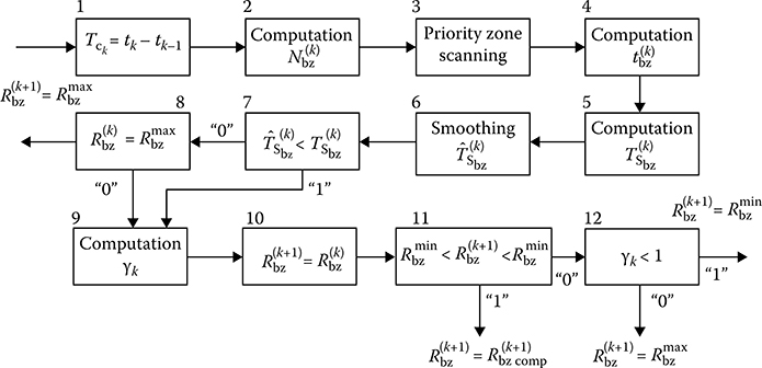
FIGURE 6.6 Flowchart of scanning control algorithm.
is the time required to scan the jth priority zone in the kth cycle with the period of
is determined by block 4. The searching period of the buffer zone based on data of the kth control cycle
where Nbz is the number of scanned directions within the limits of the buffer zone that is determined by block 5. Henceforth, the computed scan period is smoothed by the totality of some control cycles (block 6). At the same time, as a first approximation, we can assume that the scan period is changed slowly within the limits of a small observation interval, and we can use the formula for exponential smoothing in the simplest form [17]:
where ι is the constant with a sense of the smoothing coefficient lying within the limits 0 < ι < 1. In future, the scan period
If the condition (6.39) is satisfied, there is a need to check the buffer zone radar range, that is, whether
If the condition
is satisfied, block 9 computes the coefficient γk of the buffer zone radar range changing
that is,
In this case, block 10 computes the buffer zone radar range as given by
Computation of the buffer zone radar range
Otherwise, the equality (6.44). At this stage the control algorithm cycle is stopped.
There is a need to emphasize that the considered example is one of the possible ways of the scanning control algorithm subjected to analysis and comparison with other versions of scanning control algorithms in the course of designing the CRS.
6.4 Power Resource Control Under Target Tracking
6.4.1 CONTROL PROBLEM STATEMENT
The target tracking mode can be divided conditionally into two stages. The first is the pretracking stage that starts immediately after detection of new target tracing. There is a need to specialize the parameters of new target tracing in such a way that it is possible to evaluate the importance of the target (danger or not danger). In other words, there is a need to define parameters and characteristics of target movement with respect to the defended object, served airdrome of departure/arrival, or other controlled reference points. Additionally, based on obtained target tracking and signal processing data there is a need to define a predictable line of target service, for example, airdrome for air target or air-based, submarine-based, and land-based location. The required accuracy of target information to evaluate the target importance depends on the kind of target and system assigning. To reduce the time required to evaluate target importance, there is a need to select a variable location rate and the value of location rate must be as high as possible.
The second stage is that of stationary target tracking. This stage starts after evaluation of target importance and making the decision about the location of target service line. Since the qualified service and target tracking are possible only after reaching the given accuracy of target tracking estimation at the boundary line, the main task of the second stage is to accumulate information about the target tracking parameters and to extrapolate this information at the required instants, when the target tracking information is in stationary mode. Accuracy of evaluation of the target tracking parameters depends on accuracy of individual measurements of target coordinates and the number of observations (measurements). A choice of signal processing algorithm, in particular, the filtering algorithm, is very essential. In a general case, the problem is to get the required accuracy at minimal expenditure of energy and minimal digital signal processing system loading. Naturally, these requirements look as a contradiction, since increasing accuracy and target tracking subsystem reliability for real targets are possible only under more sophisticated signal processing or filtering algorithm; for example, the implementation of adaptive signal processing algorithms, which leads us to increasing the digital signal processing subsystem loading, or with increasing the frequency of coordinate measurements (increasing the number of observations or measurements), which leads us to an increase in CRS energy expenditure.
In the process of designing the CRS digital signal processing subsystem, sometimes there is a need to implement simple filtering algorithms or other kinds of simple digital signal processing algorithms with the purpose of reducing the digital signal processing subsystem loading. However, this simplification leads us to an increase in CRS energy expenditure for each tracking target. In other words, a throughput of the number of tracking targets by “CRS–digital signal processing subsystem” channel is decreased. Evidently, a simplification of digital signal processing algorithm has a sense if the additional digital signal processing subsystem loading is little and acceptable with CRS specifications.
We return again to the problem of required assurance of accuracy of target information at a target service line and discuss briefly what must be considered as a measure of this accuracy, that is, as a measure of figure of merit of target tracking problem at the considered stage. As we know, an accuracy of target tracing is characterized by the correlation matrix of errors in the definition of target tracking parameters. However, the correlation matrix of errors owing to its multidimensionality cannot be considered as a united measure of target tracking accuracy at a target service line. For this purpose, there is a need to choose any scalar factor that takes into consideration the most complete information contained in the error correlation matrix of estimation. The parameters listed here can serve as such a factor.
Determinant of the diagonal or factored correlation matrix of errors given by
where
Tracing of the correlation matrix of errors can be presented in the following form:
In this case, a high accuracy of estimation by some parameters does not make a great contribution to factor value as a whole, and an action of poor estimations by one or several coordinates is significant.
The highest eigenvalue of the correlation matrix of errors can be presented in the following form:
This factor defines some spherical estimation of error ellipsoid dimensions, since
6.4.2 EXAMPLE OF CONTROL ALGORITHM UNDER TARGET TRACKING MODE
In accordance with the adopted initial premises, the target information processing in target tracking mode is started after making a decision about new target track detection. In this mode, first of all, there is a need to accumulate information and refine the parameters to solve the problem of target classification by importance. After that, at the second stage, there is a need to organize an individual target tracking for that targets, for which a numeric measure of target importance exceeds the given threshold.
A simple logical flowchart of a digital signal processing algorithm in the case of the target tracking mode with necessary control elements using the criterion of minimization of energy expenditure and computer cost is presented in Figure 6.7. Based on the mode control algorithm commands, the antenna beam is oriented in the direction
where Trenew is the period of refreshment at the preliminary target tracking stage (block 6). After that, we compute extrapolated parameter values at the instant

FIGURE 6.7 Flowchart of digital signal processing.
If an accuracy sufficient for classification is obtained, we can assign P = 1 (the block 10) and evaluate the tactical importance of the target (block 11). The simplest factors for evaluation are the velocity and direction of target moving. The target importance Mtg is evaluated by any quantitative assessment that is compared with the threshold Mth (block 12). If the condition Mtg < Mth is satisfied, the target is assigned for the system of group target tracking using the periodical scanning data of radar coverage (block 13). If the condition Mtg > Mth is satisfied, the target is considered as the important target and an individual target tracking is organized. For this purpose, first of all, there is a need to solve an optimization problem to define the number Nsc of scans in each direction (the number of pulses in pulse train or, in other words, a volume of pulse train) and the number nsc of points of location on the target tracking from the instant of starting the individual target tracking until the instant of reaching the target service line (block 14). In a general case, the choice of the optimal values Nsc and nsc is made using the criterion of CRS power resource minimization taking into consideration restrictions assigned under the problem definition. Computation results containing the refreshment period and number of scans at each location point are registered by corresponding blocks of the digital signal processing algorithm and used for CRS operation mode schedule.
At the stage of individual target tracking, it is worthwhile to carry out a parameter filtering using a more complex digital signal processing algorithm in comparison with the previous stage, for example, the adaptive digital signal processing algorithm discussed in Chapter 5. The use of adaptive digital signal processing algorithms makes a realization of the filter F2 (block 16) more complex. However, this action allows us to keep the constant period or information update about the maneuvering target tracing at acceptable dynamical errors of smoothing. Information about the target tracing parameters goes from the adaptive filter F2 output to the display system, user (block 17), and antenna control block (block 7 and further).
Thus, in the discussed example, a direct control of important target tracing is reduced to draw a rational schedule of measurements for each target based on CRS power resource minimization. In doing so, we assume that computer costs allow us to realize the discussed control algorithm. To consider this problem in a general case, there is a need to use the following restrictions on expenditure of energy and computer costs:
The use of two-target tracking modes—the mode of individual target tracking for very important targets and the mode of target group tracking (this mode does not need additional power resources) for target, the importance of value of which is lower than the threshold
The use of the linear smoothing filter at the stage of preliminary target tracking that allows us to save computer costs
Minimization of expenditure of energy that is necessary to obtain the given accuracy at the line of getting information about the important targets
In conclusion, we can make two remarks that are useful in designing the target tracking algorithms in specific conditions.
For the two-mode CRSs discussed in detail, the target tracking process must be organized in such a way that all targets, independently of their importance, would be processed and the important targets must be processed using an individual mode additionally. In this case, the organization of digital signal processing control becomes simpler. Moreover, the reliability of important target tracking is increased. However, at the same time, the digital signal processing algorithm loading is increased.
When the given accuracy is reached, the important targets are assigned to a system of direct service. However, these targets cannot be removed from tracking mode and must be tracked and observed, at least, until when information about their full service is available or these targets leave the scanning area. The period of target refreshment for this final stage of target tracking must support precision characteristics of output parameters at the given level or to ensure a stable (without faults) target tracking.
6.4.3 CONTROL OF ENERGY EXPENDITURE UNDER ACCURACY ALIGNING
Control of target tracking mode under the same conditions is optimized by the criterion of energy expenditure minimization up to that moment when the accuracy of parameter estimation of each target coincides with the given value obtained at the line of release of information. At the same time, the duration of scanning signals τscan, the period of searching signals T, the width of directional diagram of transmit and receive antennas, the number Nsc of scans in each target location point, and the number of points of location Nl within the limits of measured interval of target tracing can be considered as controlled parameters. In practice, we try to decrease the number of controlled parameters and consider the number Nsc of scans or the volume of scanning pulse train in the course of a single determination of target coordinate. The number of measurements (updates) of target coordinates for each target track until reaching the given accuracy is considered as the controlled parameters. In this case, the problem of target tracking mode control is reduced to assign the optimal schedule of CRS operation by each target taking into consideration a set of tracking targets. The control process is an instruction issue consisting of the coordinate measurement instants
Solution of the assigned optimal control problem of target tracking mode can be delivered by mathematical programming methods (software). However, these methods are cumbersome and not always appropriate, especially, under the dynamical mode of CRS operation. Consider the simplest and, consequently, easiest to implement version of the assigned problem solution. Let the lines of release of information and the required accuracy of information release at the line be given. Let the maximal variance of estimation of the target coordinates be selected as a measure of accuracy. We assume that the target tracking is organized in such a way that a sequence of measurements is uniformly precise and equally discrete. There is a need to choose
We choose the following restrictions directly acting on the assigned optimal control problem:
The target tracing is linear within the limits of considered interval.
The minimum number
Nminscj is defined by the requirement of measure reliability, that is, the requirement to accumulate the valueSNRΣ=Nscjq21j>q2th,(6.50) at which the formulas associating a potential measure accuracy with the SNR by energy are correct [18–24], where
q21j is the SNR by energy under receiving a single target return signal from the jth target.The period of measurements is bounded up by permissible errors of target tracing extrapolation.
Further, for example, we are limited by consideration of a single angle coordinate under the target moving by circle with the constant radial velocity. In this case, the potential measure accuracy is given by
where ℒac is the coefficient taking into consideration losses under the accumulation process. If we know CRS characteristics and parameters, targets, noise, and interferences, then
On the other hand, when our measurements are uniformly precise and equally discrete, the variance of filtering error of linear target track coordinates is determined by the following formula (see Chapter 5):
In the considered case, we must satisfy the condition
where
Thus, we have a relation between the unknown parameters
In this case, the optimal control problem is reduced to selection of the pair
Computation is easy and can be done in real time. Figure 6.8 represents the results of computation (6.57). CRS energy parameters are presented conditionally by the SNR by energy under a single measurement. As we can see from Figure 6.8, in the considered case, there is a need to select the permissible minimum number Nsc and calculate the corresponding number Nl to optimize the target tracking process since an increase in accuracy of a single measurement leads us to increase in total losses K. Thus, the optimization of the tracking mode of the jth target based on the considered criterion is reduced, in the simplest case, to performing two operations:
Based on SNR by energy, there is a need to compute the number of scanning signals
Nscj to satisfy the conditionσ2θˆj≤σ2θˆjaccept .Knowledge of
σ2θˆjaccept andσ2θˆj allows us to computeN1j using (6.53).

FIGURE 6.8 Results of computation based on (6.57).
6.5 Distribution of Power Resources of Complex Radar System Under Combination of Target Searching and Target Tracking Modes
When CRSs work in the mode of individual important target tracking detecting a new target simultaneously, the problem of optimal distribution of limited power resources between these modes arises. In this case, the criterion of optimal distribution must take into account the quality factor of digital signal processing for each mode, for example, a maximization of the tracking targets number with the given precision characteristics at information issue lines with simultaneous detection of new targets with the given probability of detection PD at the given line; an assurance of qualitative (with the user view point) target tracking of the given number of targets and minimization of target detection time in searching mode, simultaneously.
In a general case, a solution of the problem of optimal distribution of power resources between the target scanning modes and target tracking is absent. In this section, we consider one of the possible engineering approaches to the distribution problem of power resources of the two-mode CRS with programming control of the antenna directional diagram beam. In the simplest case, when there are no zones with the high a priori probability of new target appearance in the radar coverage, the target tracking mode is considered as priority mode and, consequently, all requirements of this mode for CRS power resource consumption are satisfied in the first place. In this case, the remaining power resources are used for the new target searching mode. The limitation for maximum permissible period of scanning
When the number of tracked target is small, an excess of energy is spent to reduce the period of radar coverage scanning and, consequently, used to improve conditions of new target detection. As the number of tracked target increases, the energy consumption for target tracking increases and under definite task conditions can reach such a value when a remainder of CRS power resources assigned for searching new targets cannot satisfy the condition
Now, let us define the elementary relations allowing us to reach a balance of CRS power resources at two-mode operation. Let targets be tracked under the ith scanning Mi. Denote
as the power resource expressed by the time of direction scanning spent on a single coordinate measurement of the jth target under the ith scanning; j = 1, 2,…, Mi,
Let the number of directions that must be scanned within the limits of radar coverage be Nd, and the number of targets inside the radar coverage at the ith scanning is subjected to the condition
where
τ¯n is the average time of directional analysis, in which there are no targets (the noise direction)τ¯scan is the average time of directional analysis, in which there are targets
Now, based on the condition
we can define the scanning time at the ith scanning of radar coverage:
If the obtained scanning time satisfies the following condition
Now, consider a general case of the distribution problem for limited CRS power resources. Let there be several zones in the radar coverage, namely, Z1, Z2,…, Zl for which the periods
The part of CRS power resources required for scanning of the kth zone is given by
where
ttotalki¯¯¯¯¯¯ is the average time required to scan the priority zone at the ith scanning computed analogously as in (6.30)Ttotalk is the assigned period of scanning for the kth zone
The part of CRS power resources required to scan all priority zones at the ith scanning is determined by
As a result, the part of CRS power resources remaining to scan the no priority l + 1th zone is determined by
In turn,
where
ttotal(l+1)i is the time required to scan the no priority l + 1th zone at the ith scanningTtotal(l+1)i is the period of the ith scanning for the l + 1th zone
Thus, in the given case, the scanning period
If the condition
6.6 Summary and Discussion
The radar engineer has a resource time that allows good Doppler processing, bandwidth for good range resolution, space that allows a large antenna, and energy for long-range performance and accurate measurements. External factors affecting radar performance include the target characteristics; external noise that might enter via the antenna; unwanted clutter echoes from land, sea, birds, or rain; interference from other electromagnetic radiators; and propagation effects due to the Earth’s surface and atmosphere. These factors are highly important in CRS design and application.
The hierarchy of the control process is characterized by a sequential release of information from a complex radar subsystem of higher level to lower level subsystems. At the same time, the results of particular problem solutions at lower levels are used as the basis to make decisions at the higher level. Thus, information about the energy consumption for scanning in each direction, the number of detected targets, and the energy consumption under target tracking mode comes to the second-level subsystem as a result of the first-level task solutions. The information about the number of tracked targets
Under directional scanning in the mode of searching new targets, the control process is carried out by two stages. At the first stage, the calculation and choice of scanning signal parameters are carried out. The scanning signals must correspond to the functional mode of searching targets and maximal radar range in the given direction. Additionally, the receiver performance and signal processing algorithms for signal preprocessing subsystems should be defined and computed. This stage is carried out before scanning pulsing in the given direction. The control of accumulated received signals up to making decisions about the target detection/nondetection using all resolution elements in the radar range (the case of sequential analysis) or up to accumulation of determined number of the target return signals using detectors with the fixed sample sizes is carried out at the second stage. In the course of accumulation of the target return signals, the initial parameter values of scanning signals are the same except the carrier frequency fc (see Figure 6.3).
After finishing the accumulation stage and making a decision about the scanned direction, the results of decision making are issued and expenditure of energy and timetable are computed to observe the scanned direction (block 9, Figure 6.3). The radar antenna beam control is assigned for an algorithm of scanning management in the searching mode or mode controller. In conclusion, we note once more that the discussed logical flowchart is the way only to assign a control process under the searching new target mode. Naturally, there are possible other ways, but a general idea to control, namely, parametric matching of CRS subsystems and signal and data processing subsystems with environmental parameters and solved problems and tasks, is the same.
The control algorithm under refreshment of target in target tracing mode operates interactively in a close way with algorithms of the main operations of signal preprocessing and reprocessing subsystems within the limits of the gate coordinating these algorithms into the unique signal processing subsystem in the individual target tracking mode by CRS with the control beam of radar antenna directional diagram.
In radar, a control process is based on to obtain the radar coverage scanning, selection of angle direction and interval on radar range scanning, shape of radar antenna directional diagram, type of searching signal, and so on. In our case, a control process of scanning is reduced to control the radar antenna directional diagram position, the shape and angle dimensions of which are fixed under the condition of realization of the discussed algorithms. Under synthesis of observation control algorithms, it is natural to follow the principle of the average risk minimization, that is, minimization of losses arising under the decision error. However, in this case, a choice of the corresponding function of losses is a very hard problem. The approximate approach is based on a set of assumptions, the important of which are the following: the problem is solved for a single target or set of uncorrelated targets; the observation space consists of cells and we can scan a single cell only within the limits of observation step (the scanning period); in this case, a control process is the integer scalar value υ coinciding with the number of observed cell; and the υth cell random value X observed under scanning is a scalar and subjected to the pdf p0(x) in the case when the target is absent and the pdf p1(x) if the target is present; these pdfs are considered as known.
The main result of analysis of optimal control methods to scan a single target within the limits of radar coverage consisting of N cells is the optimal control algorithm of radar coverage scanning that is reduced to get the a posteriori probabilities Pt(i) of target presence in the cells (i = 1, 2,…, N) and to select the cell for next scanning (i = υ), within the limits of which the a posteriori probabilities Pt(i) of target presence are maximal, that is,
As a model of radar coverage situation, we consider an uncorrelated set of targets that appear and move within the limits of the radar coverage (from cell to cell) independently of each other. The probability of a presence in each cell of more than one target is equal to zero, which corresponds to a model of rarefied flow. As earlier, the probability of target appearance in the ith cell during the time τ is equal to Pτ(i) and replacement of targets from cell to cell is described by the passing probability Pτ (i | j). A procedure of optimal scanning is to choose that cell at the next step, for which the a posteriori probability of target presence is maximal. However, the following fact plays a very important role in this procedure: there are several targets within the limits of radar coverage. By this reason, there is a need to ensure a mode of sequential addressing to different cells including the cells with the minimal probability of target presence. Thus, the control algorithm ensures a sequential addressing to the cells including the cells with the low a posteriori probability of target presence. The considered algorithm is optimal based on the viewpoint of minimization of the number of scanning cycles T from the beginning to scan to the instant of detection of all targets. We have a principal possibility to design and realize the optimal control algorithm for scanning under detection of targets within the radar coverage. However, realization of such algorithms in practice is very difficult. Difficulties are caused by the methodological and computational peculiarities.
In practice, in designing the control subsystem of signal processing and CRS operation we should proceed from the simplest assumptions about spatial searching and distribution of target in this space. First, we assume that the searching space consists of uniform searching zones, within the limits of which the target situation is of the same kind. The intensity of target set in each zone can be estimated a priori based on purposes of the CRS and conditions to exploit it. The probabilities of target presence in each direction of the selected scanning zone are considered as the same, and the noise regions are assumed to be localized. Because of this, there are no priority directions to search for the targets and the zone scanning is carried out sequentially and uniformly with the period TS. In this case, the problem of controlling the scanning is to optimize the zone scanning period, for example, using the criteria to minimize the average time when the target could enter the scanning zone until the target detection under limitations in power resources issued to detect new targets.
When CRSs work in the mode of individual important target tracking detecting a new target simultaneously, the problem of optimal distribution of limited power resources between these modes arises. In this case, the criterion of optimal distribution must take into account a quality factor of digital signal processing for each mode, for example, a maximization of the tracking targets number with the given precision characteristics at information issue lines with simultaneous detection of new targets with the given probability of detection PD at the given line; an assurance of qualitative (with the user view point) target tracking of the given number of targets and minimization of target detection time in searching mode, simultaneously.
When the number of tracked target is small, an excess of energy is spent to reduce the period of radar coverage scanning and, consequently, used to improve conditions of new target detection. As the number of tracked targets increases, the energy consumption for target tracking increases and under definite task conditions can reach such a value when a remainder of CRS power resources assigned for searching new targets cannot satisfy the condition
References
1. Scolnik, M. 2008. Radar Handbook. 3rd edn. New York: McGraw Hill, Inc.
2. Scolnik, M. 2002. Introduction to Radar Systems. 3rd edn. New York: McGraw Hill, Inc.
3. Hansen, R. C. 1998. Phased Array Antenna. New York: John Wiley & Sons, Inc.
4. Mailloux, R.J. 2005. Phased Array Antenna Handbook. Norwood, MA: Artech House, Inc.
5. Cantrell, B., de Graaf, J., Willwerth, F., Meurer, G., Leibowitz, L., Parris, C., and R. Stableton. 2002. Development of a digital array radar. IEEE AEES Systems Magazine, 17(3): 22–27.
6. Scott, M. 2003. Sampson MFR active phased array antenna, in IEEE International Symposium on Phased Array Antenna Systems and Technology, October 14–17, Boston, Massachussets, Isle of Wight, U. K., pp. 119–123.
7. Brookner, E. 2006. Phased arrays and radars—Past, present, and future. Microwave Journal, 49(1): 24–46
8. Brookner, E. 1988. Aspects of Modern Radar. Norwood, MA: Artech House, Inc.
9. Wehner, D. R. 1995. High-Resolution Radar. 2nd edn. Boston, MA: House, Inc.
10. Nathanson, F. E. 1991. Radar Design Principles. 2nd edn. New York: McGraw-Hill, Inc.
11. Rastrigin, L. A. 1980. Modern Control Principles of the Complex Objects. Moscow, Russia: Soviet Radio.
12. Picinbono, B. 1993. Random Signals and Noise. Englewood Cliffs, NJ: Prentice-Hall, Inc.
13. Porat, B. 1994. Digital Processing of Random Signals. Englewood Cliffs, NJ: Prentice-Hall, Inc.
14. Therrein, C.W. 1992. Discrete Random Signals and Statistical Signal Processing. Englewood Cliffs, NJ: Prentice-Hall, Inc.
15. Bacut, P. A., Julina, Yu.V., and N. A. Ivanchuk. 1980. Detection of Moving Targets. Moscow, Russia: Soviet Radio.
16. Kontorov, D. S. and Yu.S. Golubev-Novogilov 1981 Introduction to Radar Systems Engineering Moscow, Russia: Soviet Radio.
17. Kuzmin, S.Z. 1974. Foundations of Radar Digital Signal Processing Theory. Moscow, Russia: Soviet Radio.
18. Helstrom, C.W. 1995. Elements of Signal Detection and Estimation. Upper Saddle River, NJ: Prentice-Hall, Inc.
19. Levanon, N. and E. Mozeson. 2004. Radar Signals. New York: John Wiley/IEEE Press.
20. Middleon, D. 1996 An Introduction to Statistical Communication Theory New York: McGraw-Hill. Reprinted by IEEE Press, New York.
21. Kay, S. M. 1998. Fundamentals of Statistical Signal Processing: Detection Theory. Englewood Cliffs, NJ: Prentice-Hall, Inc.
22. Levanon, N. 1988. Radar Principles. New York: John Wiley & Sons, Inc.
23. Di Franco, J.V. and W. L. Rubin. 1980. Radar Detection. Norwood, MA: Artech House, Inc.
24. Carrara, W. G., Goodman, R. S., and R. M. Majewski. 1995. Spotlight Aperture Radar—Signal Processing Algorithms Norwood, MA: Artech House, Inc.