
4 Algorithms of Target Range Track Detection and Tracking
Target range tracking is accomplished by continuously measuring the time delay between the transmission of an RF pulse and the echo signal returned from the target and converting the roundtrip delay into units of distance. The range measurement is the most precise position-coordinate measurement of the radar; typically, with high SNR, it can be within a few meters at hundreds-of-kilometers range. Range tracking usually provides the major means for discriminating the desired target from other targets, although the Doppler frequency and angle discrimination are also used, by performing range gating (time gating) to eliminate the echo of other targets at different ranges from the error detector outputs. The range-tracking circuitry is also used for acquiring a desired target. Target range tracking requires not only that the time of travel of the pulse to and from the target be measured but also that the target return signal is identified as a target rather than noise and a range-time history of the target be maintained.
Although this discussion is for typical pulse-type tracking radars, the target range measurement may also be performed with continuous wave (CW) radar systems using the frequency-modulated continuous wave (FM-CW) that is typically a linear-ramp FM. The target range is determined by the range-related frequency difference between the echo-frequency ramp and the frequency of the ramp being transmitted. The performance of FM-CW radar systems, with consideration of the Doppler effect, is discussed in Ref. [1].
Acquisition: The first function of the target range tracker is acquisition of a desired target. Although this is not a tracking operation, it is a necessary first step before the target range tracking or target angle tracking (the azimuth tracking) may take place in a typical radar system. Some knowledge of target angular location (the target azimuth) is necessary for pencil-beam tracking radar systems to point their typically narrow antenna beams in the direction of the target. This information, called designation data, may be provided by surveillance radar systems or some others. It may be sufficiently accurate to place the pencil beam on the target, or it may require the tracker to scan a larger region of uncertainty. The range-tracking portion of the radar has the advantage of seeing all targets within the beam from close range out to the maximum range of the radar. It typically breaks this range into small increments, each of which may be simultaneously examined for the presence of a target. When beam scanning is necessary, the target range tracker examines the increments simultaneously for short periods, such as 0.1 s, makes its decision about the presence of a target, and allows the beam to move to a new location if a “no” target is present. This process is typically continuous for mechanical-type trackers that move the beam slowly enough that a target will remain well within the beam for the short examination period of the range increments.
Target acquisition involves consideration of the S/N threshold and integration time needed to accomplish a given probability of detection PD with a given false alarm rate PF similar to surveillance radar system. However, the high false alarm rates PF, as compared with values used for surveillance radar systems, are used because the operator knows that the target is present, and operator fatigue from false alarms when waiting for a target is not involved. Optimum false alarm rates PF are selected on the basis of performance of electronic circuits that observe each range interval to determine which interval has the target echo.
A typical technique is to set a voltage threshold sufficiently high to prevent most noise peaks from crossing the threshold but sufficiently low that a weak signal may cross. An observation is made after each transmitter pulse as to whether, in the range interval being examined, the threshold has been crossed. The integration time allows the radar to make this observation several times before deciding if there is a “yes” target. The major difference between noise and target echo is that noise spikes exceeding the threshold are random, but if a target is present, that is, a “yes” target, the threshold crossings are more regular. One typical radar system simply counts the number of threshold crossings over the integration period, and if crossings occur for more than half the number of times that the radar has transmitted, a target is indicated as being present. If the radar pulse repetition frequency is 300 Hz and the integration time is 0.1 s, the radar will observe 30 threshold crossings if there is a strong and steady target. However, because the echo from a weak target combined with noise may not always cross the threshold, a limit may be set, such as 15 crossings, that must occur during the integration period for a decision that is a “yes” target. For example, performance on a nonscintillating target has a 90% probability of detection PD at a 2.5 dB per-pulse SNR and the false alarm probability PF = 10−5.
Target range tracking: Once a target is acquired in range, it is desirable to follow the target in the range coordinate to provide distance information or slant range to the target. Appropriate timing pulses provide a target range gating so the angle-tracking circuits and automatic gain control (AGC) circuits look at only the short target range interval, or time interval, when the desired echo pulse is expected. The target range tracking operation is performed by closed-loop tracking similar to the azimuth tracker. Error in centering the range gate on the target echo pulse is sensed, error voltages are generated, and circuitry is provided to respond to the error voltage by causing the gate to move in a direction to recenter on the target echo pulse.
Automatic target range tracking can generally be divided into five steps shown in Figure 4.1 and detailed here:
Radar detection acceptance: Accepting or rejecting detections for insertion into the tracking process. The purpose of this step is to control the false track rates.
Association of accepted detections with the existing tracks.
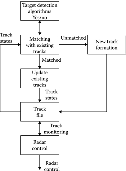
FIGURE 4.1 Target range tracking procedure.
Updating the existing tracks with associated detections.
New track formation using unassociated detections.
Radar scheduling and control.
The result of the automatic target range tracking is the track file that contains a track state for each target detected by the radar system. As shown in Figure 4.1, there is a feedback loop between all these functions, so the ability to update existing tracks accurately, naturally, affects the ability to associate detections with existing tracks. Also, the ability to correctly associate detections with existing tracks affects the track’s accuracy and the ability to correctly distinguish between an existing track and a new one. The detection accept/reject step makes use of feedback from the association function that measures the detection activity in different regions of the radar coverage. More stringent acceptance criteria are applied in more active regions.
When a track is established in the computer, it is assigned a track number. All parameters associated with a given track are referred to by this track number. Typical track parameters are the filtered and predicted position; velocity; acceleration (when applicable); time of last update; track quality; SNR; covariance matrices (the covariance contains the accuracy of all rank coordinates and all the statistical cross-correlations between them), if a Kalman-type filter is being used; and track history, that is, the last n detections. Tracks and detections can be accessed in various sectored, linked-list, and other data structures so that the association process can be performed efficiently [2-4]. In addition to the track file, a clutter file is maintained. A clutter number is assigned to each stationary or very slowly moving echo. All parameters associated with a clutter position are referred to by this clutter number. Again, each clutter number is assigned to a sector in azimuth for efficient association.
When the radar system has either no or limited coherent processing, not all the detections declared by the automatic detector are used in the tracking process. Rather, many of the detections (contacts) are filtered out in software using a process called activity control [5,6]. The basic idea is to use detection signal characteristics in connection with a map of the detection activity to reduce the rate of detections to one that is acceptable for forming tracks. The map is constructed by counting the unassociated detections (those that do not associate with existing tracks) at the point in the track processing shown in Figure 4.1.
4.1 Main Stages and Signal Reprocessing Operations

FIGURE 4.2 Target detection and target range tracking coordinate system.
The signal reprocessing operations of each target are carried out in two stages [7,8]: the target range track detection and the target range tracking. Automatic target range track detection using data of 2D radar system in the Cartesian rectangular coordinates under uniform radar antenna scanning is shown in Figure 4.2. Let a target pip be at any point of uniform radar antenna scanning area that does not correspond to existing target range tracks. This target pip is considered as a target range track datum of new target. If components by coordinate axes of minimal Vmin and maximal Vmax target velocities are known, then the area S1 within the limits of which we should search the second target pip during next radar antenna scanning can be presented as an area between two rectangles. In doing so, the internal rectangle sides are defined as 2VXmin Tscan and 2VY min Tscan; the external rectangle sides are defined as 2VXmax Tscan xand 2VY max Tscan, where Tscan is the radar antenna scanning period. The operation forming the area S1 is called a gating and the area S1 is called a gate with primary lock-in.
Several target pips may be in the gate with primary lock-in. Each target pip must be considered as one of the possible prolongations of existing target range tracks (see Figure 4.2). Using two target pips we can compute the velocity and direction of target moving and then determine a possible position of target pip for next (third) radar antenna scanning. The definition of initial parameters, namely, the velocity, target moving direction, and extrapolation of target pip position for the next radar antenna scanning, is realized by specific filtering (see Chapter 5). The extrapolated target pips are noted by triangles in Figure 4.2. Rectangle gates S2 are formed around the extrapolated target pips. Dimensions of these rectangle gates S2 are defined based on possible errors during extrapolation and determination of the target pip coordinates. If in the course of the third radar antenna scanning we can observe the definite target pip within the limits of the rectangle gate S2, then we can think that this target pip belongs to the detected target range track. Taking into consideration the coordinates of this target pip we are able to obtain more specific information about target range track parameters and construct new rectangle gates. After performance of the earlier-given criterion by number of target pips that are within l consistently formed rectangle gates, we accept a detection and start a procedure of target range tracking. As follows from Figure 4.2, the detection is accepted based on three target pips following one after another—the criterion “3 from 3.” Thus, in the course of target range track detection, the following operations are made:
Gating and selection of target pip within the gate
Checking the detection criterion
Estimation and extrapolation of target range track parameters
Target range tracking is a sequential from measuring to measuring procedure of newly obtained target pip binding to target range track and accurate target range track determination. Under target range autotracking, the following operations are carried out:
Accurate definition of target range track parameters in the course of newly obtained target pip binding
Extrapolation of target range track parameters for next radar antenna scanning
Range gating of possible newly obtained target pip positions
Selection of the definite target pip within the gate if there are several target pips within the gate area
When there are several target pips within the tracking gate, we expand the target range track binding for each target pip. When the target pip is absent within the tracking gate, the target range track is prolongated by the corresponding extrapolated point, but the next gate is increased in area to take into consideration the errors increasing in the course of extrapolation. If there are no target pips during k radar antennas scanning following one after another, the target range tracking is canceled. Thus, at the stages of target range track detection and target range tracking, we carry out the same operations in reality:
Radar antenna scanning area gating
Selection and identification of target pips within the gate
Filtering and extrapolation of target range track parameters
Consider algorithms of the first and second operations.
4.1.1 TARGET PIP GATING; SHAPE SELECTION AND DIMENSIONS OF GATES
In accordance with the main principles of target range autotracking, a newly obtained target pip can be used to suggest a target range tracking if a target pip deviation from the gate center does not exceed a given before fixed value defined by gate dimensions or, in other words, if the following condition is satisfied:
|Ui−ˆUcenteri|≤0.5ΔUgatei,(4.1)
where
Ui={ri,βi,εi}(4.2)
is a set of coordinates of the ith newly obtained target pip;
ˆUcenteri={ˆrcenteri,ˆβcenteri,ˆεcenteri}(4.3)
is a set of the gate center coordinates for the ith target range track;
ΔUgatei={Δrgatei,Δβgatei,Δεgatei}(4.4)
are the gate dimensions by coordinates r, β, and ε for the ith target range track. One of the problems arising during the prolongation of the target range tracks by gating is a problem of selection of gate shape and dimensions based on known statistical characteristics of deviations of true (belonging to prolongated target range tracks) target pips from their corresponding extrapolated points. Deviation of the true target pip from the gate center is defined by total (random plus dynamic) errors of target coordinate extrapolation by previous smoothed parameters of target range track and coordinate measurement errors of newly obtained target pips. These errors are independent and identically distributed, subjected to the normal Gaussian pdf.
Let the target range track coordinate extrapolation for the next nth radar antenna scanning be carried out using the data of previous (n- 1)th radar antennas scanning. Position of the extrapolated point is denoted by O (see Figure 4.3). We think that the origin of Cartesian coordinate system is located at the point O. The axis Y is matched with “radar system-target” direction, the axis X is a perpendicular to the “radar system-target” direction away from radar antenna rotation, and the axis Z is directed in such way that we have a right-handed coordinate system. Then the random deviations Δx, Δy, Δz of the newly obtained under nth radar antenna scanning target pip from the gate center are defined in the following form:
{Δxn=±r(Δβextrn+Δβn)Δyn=±(Δrextrn+Δrn)Δzn=±r(Δεextrn+Δεn)(4.5)
where
Δrextrn,Δβextrn
Δrextrn,Δβextrn , and ΔεextrnΔεextrn are the random errors of coordinate extrapolation in the course of the nth radar antenna scanningΔrn, Δβn, and Δεn are the random errors of coordinate measuring in the course of the nth radar antenna scanning
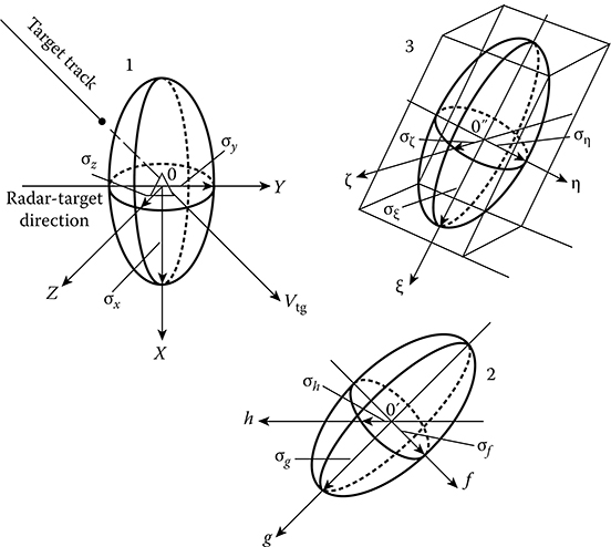
FIGURE 4.3 Extrapolation of target coordinates.
Under the definition of gate dimensions we can believe that the components Δrn, Δβn, and Δεn are statistically independent, do not depend on the scanning number step n, and are subjected to the normal Gaussian pdf with zero mean and variances σ2x,σ2y
f(Δx,Δy,Δz)=1√(2π)3σ2xσ2yσ2zexp{−12[(Δx)2σ2x+(Δy)2σ2y+(Δz)2σ2z]},(4.6)
and the surface corresponding to equal pdf is defined by the following equation:
(Δx)2σ2x+(Δy)σ2y+(Δz)2σ2z=λ2,(4.7)
where λ is the arbitrary constant. Dividing the left- and right-hand side of (4.7) by λ2, we obtain
(Δx)2λ2σ2x+(Δy)2λ2σ2y+(Δz)2λ2σ2z=1.(4.8)
Equation 4.8 is the ellipsoid equation with conjugate axles λσx, λσy, and λσz. At λ = 1, we obtain the unit ellipsoid—see ellipsoid 1 in Figure 4.3.
Henceforth, we believe that dynamical errors of extrapolation caused by contingency target maneuver are also normally distributed and have independent components on the F, G, and H axes. The F axis is matched with the target velocity vector; the G axis is directed in opposition to a tangential acceleration; and the H axis supplements the system to the right-handed coordinate one. Origin of the obtained coordinate system, as well as in the case of the previous coordinate system, coincides with the extrapolated point O. For better visualization the origin is replaced at the point O′ in Figure 4.3.
In 3D space the dynamic errors form an ellipsoid of equal probabilities, an equation of which takes the following form:
(Δf)2λ2σ2f+(Δg)2λ2σ2g+(Δh)2λ2σ2h=1,(4.9)
the ellipsoid 2 in Figure 4.3 at λ = 1. If we add ellipsoids 1 and 2, then ellipsoid 3 will be formed, and directions of conjugate axles (the directions of axes of the Cartesian coordinate system Oηξζ with respect to the axes of the Cartesian coordinate system OXYZ and variances σ2η,σ2ξ
The joint pdf of random components Δη, Δξ, and Δζ takes the following form:
p(Δη,Δξ,Δζ)=1√(2π)3σ2ησ2ξσ2ζexp(−0.5λ2),(4.10)
where
λ2=(Δη)2σ2η+(Δξ)2σ2ξ+(Δζ)2σ2ζ.(4.11)
Thus, a surface of equally probable deviation of true target pips from the gate center represents an ellipsoid, value and direction of conjugate axles of which relative to the direction “radar system-target” depend on coordinate measurement errors, target maneuver intensity, and vectorial direction of target moving. Under ellipsoid distribution of true target pip deviation from the gate center, it is evident that the gate must have an ellipsoid shape with the conjugate axles λση, λσξ, and λσζ, where λ is the enlargement factor of the gate dimensions in comparison with the dimensions of unit ellipsoid to ensure the given before expectancy of hitting of true target pip within the gate.
The expectancy of random point hitting into the ellipsoid that is similar and has a similar disposition as ellipsoids of equal probabilities is defined in the following form:
P(λ)=2[Φ0(λ)−1√2πλexp(−0.5λ2)],(4.12)
where Φ0(λ) is the standard normal Gaussian pdf given by (3.110). At λ ≥ 3, the probability P(λ) is very close to unit. There is a need to choose just the values of λ, forming an ellipsoid gate.
In practice, forming the ellipsoidal gates is impossible both under physical and mathematical gating. By this reason, the best thing that can be done is to form a gate in the shape of parallelepiped defined around the total error ellipsoid, as shown in Figure 4.3 (3). Parallelepiped side dimensions are equal to 2λση, 2λσξ, and 2λσζ and its volume is defined as
Vpar=8λ3σησξσζ.(4.13)
Taking into consideration the fact that the volume of total error ellipsoid is defined as
Vel=43πλ3σησξσζ,(4.14)
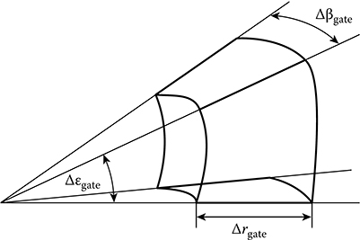
FIGURE 4.4 Definition of the simplest gate.
the gate volume is increased twice in comparison with the optimal volume. This phenomenon leads to an increase in the expectancy of hitting of false target pips within the gate or an increase in the number of target pips belonging to another target range tracks and, consequently, to deterioration of selection and resolution during gating operation.
During the processing of high number of targets in real time by the computer subsystem of a complex radar system (CRS), computation of dimensions and orientation of parallelepiped gate sides is very cumbersome. In this case, there is a need to use a simple version of gating, a sense of which is the following. The simplest gate shape is chosen for definition in that coordinate system, in which radar information is processed. In the case of spherical coordinate system, the simplest gate is given by linear dimension in target range Δrgate and by two angular dimensions, namely, by the azimuth Δβgate and elevation Δεgate (see Figure 4.4).
These dimensions can be preset based on maximal magnitudes of random and dynamic errors while processing all target range tracks. In short, in this case, the gate dimensions are chosen so that the ellipsoid of all possible (under all directions of target moving and fight) total deviations of true target pips from corresponding extrapolated points will be easily fit and rotated in any direction inside the gate. This is the crudest technique of gating. In conclusion, we note that all procedures, which are discussed in this subsection, to choose dimensions of 3D gate can be used in full during gating in plane for binding newly obtained target pips in 2D radar systems.
4.1.2 ALGORITHM OF TARGET PIP INDICATION BY MINIMAL DEVIATION FROM GATE CENTER
We consider a case of target pip indication under definition of target range track for a single target. At the same time, we assume that in addition to true target pips, the false target pips caused by noise and interferences passed over preprocessing filters can be present within the gate. Given the earlier-provided situation, the following varied decisions could be made:
When there are several target pips, there is a need to continue to define the target range tracks using each target pip; in other words, we can suppose multiple target range tracks. Prolongation of target range tracks using false target pips will be canceled over several radar antennas scanning owing to absence of confirmations, but prolongation of the target range tracks using the true target pips will be continued. Such way of newly obtained target pip binding is very tedious. Moreover, when the density of false target pips is high, an avalanche-like increase in false target tracks leading to overload of memory devices in computer subsystems is possible.
We must choose a single target pip within the gate, and we should be sure that the probability of the event that this target pip belongs to the target range tracking is the highest. Other target pips can be rejected as false. Such approach is appropriate with a view to decreasing the computation cost, but it requires a solution for the optimal target pip indication problem.
Optimization of the target pip indication process by deviation from the gate center is carried out using a criterion of maximal likelihood, on the basis of which we believe that the likelihood function is maximal only for the true target pip. Under target pip indication within 3D gate with facets that are parallel to the main axles of the total error ellipsoid (see Figure 4.3), a condition of maximal likelihood takes the following form:
ℒ(Δηitrue,Δξitrue,Δζitrue)=maxi{ℒ(Δηi,Δξi,Δζi)},(4.15)
where itrue is the number of target pip considered as true, i = 1,2, …, m, m being the number of target pips within a gate. Condition given by (4.15) is equivalent to the condition
λ2itrue=mini[(Δηi)2σ2ηi+(Δξi)2σ2ξi+(Δζi)2σ2ζi].(4.16)
Consequently, we should take into consideration only that target pip to prolong the target range track, the elliptical deviation of which from the gate center is minimal. A natural simplification of optimal operation discussed is indicated by the minimum of squared sums of linear deviations of the target pip from the gate center that corresponds to an assumption about the equality of the variances σ2ηi,σ2ξi
κ2itrue=mini[Δr2i+(riΔβi)2+(riΔεi)2].(4.17)
A quality of the target pip indication process can be evaluated by the probability of correct indication, in other words, the probability of event that the true target pip will be indicated to prolong the target range track in the next radar antennas scanning. The problem of definition of the probability of correct indication can be solved analytically if we assume that a presence of false target pips within the gate is only caused by stimulus of the noise and interference and these target pips are uniformly distributed within the limits of radar antenna scanning area. Under indication within 2D rectangle gate circumscribed around the ellipse with the parameter equal λmax ≥ 3, the probability of correct indication is determined by [9,10]
Pind=11+2πρsσησξ,(4.18)
where
ρS is the density of false target pips per unit square of gate
ση and σξ are the mean square deviations of true target pips from the gate center along the axes η and ξ
In the case of target pip indication in 3D gate that can be presented in the form of parallelogram circumscribed around the total error ellipsoid (see Figure 4.3), the probability of correct indication is determined by
Pind≈121.33πσησξσζρv√2π,(4.19)
where ρv is the density of false target pips per unit volume of gate.

FIGURE 4.5 Algorithm of target pip indication within 2D gate.
The algorithm of target pip indication within 2D gate using a minimal linear deviation from the gate center and the polar coordinate system is represented in Figure 4.5. Blocks that are not related to the algorithm are shown by the dashed line. Sequence of operations in the considered algorithm is the following.
Step 1: Using signal processing results of the previous (n − 1)th radar antenna scanning, we are able to define and compute the gate dimensions for the next nth radar antenna scanning. For choosing the gate dimensions, we should take into consideration the information about target maneuver and target pip misses.
Step 2: We select the target pips within the gate (block 2, Figure 4.5) using the following formulae:
{|Δr(i)n|=|r(i)n−ˆr(i)extrn|≤0.5Δrgaten|Δβ(i)n|=|β(i)n−ˆβ(i)extrn|≤0.5Δβgaten(4.20)
and determine their number. If there is a single target pip within the gate (m = 1), then this target pip is considered as true and comes in both at the filter input and at the input of the block of target range track parameters extrapolation (the block 5). If there are several target pips within the gate, then all of them come in at the input of computer block 3 that carries out computations of squared distances between the each target pip and the gate center by the following formula:
(d(i)n)2=(Δr(i)n)2+(r(i)nΔβ(i)n)2,(4.21)
where i = 1, 2, … m, m being the number of indicated target pips within the gate.
Step 3: We compare the squared distances (the block 4) and choose the only target pip, for which
(d(i)n)2=d2min.(4.22)
Step 4: If there are no target pips within the gate, we check the criterion of cancellation of target range tracking (the block 6). If the criterion is satisfied, then the target range tracking is canceled. If the criterion of cancellation is not satisfied, then a command to continue to expand the target range tracking by extrapolation of target range track coordinates and target range track parameters is generated.
In conclusion, we can note that in addition to target pip deviations from the gate center, the weight features of target pips formed in the course of signal preprocessing, as some analog of SNR, can be used to indicate the target pips. In the simplest case of a binary quantized target return pulse train, we can use the number of train pulses or train bandwidth to generate the target pip weight features. Weight features of target pips can be used under target range track indication jointly with features of target pip deviations from the gate center or independently. One of the possible ways to use the target pip weight features jointly with the target pip deviations from the gate center is the following. All target pips within the gate are divided on the target pips with the weight v1 and target pips with the weight v0 depending on either the target return pulse train bandwidth exceeds the earlier-given threshold value or not, which depends on target range magnitude. If there are target pips with weight v1, we indicate the target pip nearest to the gate center as the true target pip from observed target pip group. If there are no target pips with weight v1, we indicate the target pip with weight v0 nearest to the gate center as the true target pip. If we can characterize the target pip weight by the number of pulses in the target return pulse train, then we are able to indicate the target range track by the maximum number of pulses. In this case, features of target pip deviations from the gate center are only used under the equality of weights of several target pips.
4.1.3 TARGET PIP DISTRIBUTION AND BINDING WITHIN OVERLAPPING GATES
In the hard noise environment, several gates formed around extrapolated points of prolonged target range tracks will overlap. Moreover, false and newly obtained target pips will appear within gates. In this case, the problem of newly obtained target pip distribution and binding to target range tracking becomes more complex. In addition, the problem of fixing a beginning of new target range track arises. First of all, this complication is associated with the necessity to use a joint target pip binding to target range track after getting newly obtained target pips liable to binding or, in other words, if these newly obtained target pips are within overlapping gates. Henceforth, there is a need to generate all possible ways or hypotheses for target pip binding and choose the most plausible version.
Consider one approach to solve the problem of target pip distribution and binding in overlapping gates under the following initial premises:
The gates formed by each target range track have such dimensions that the probability of hitting of true target pips belonging to the given target range track is very close to unit.
Groups of overlapping gates are selected in such way that each group can be processed individually.
The problem is solved within 2D gates.
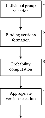
FIGURE 4.6 Target pip distribution and binding algorithms.
A logical flowchart of target pip distribution and binding algorithm within the isolated group of overlapping gates is presented in Figure 4.6. Block 1 selects the isolated groups with overlapping gates. Block 2 generates possible target pip binding versions taking into account information about the sources of newly obtained target pips forming a group. The following hypotheses are considered with respect to each target pip: The first hypothesis is that the target pip belongs to an earlier-detected target range track or to a new target range track, and the second hypothesis is that the target pip is false. Block 3 computes probabilities of all versions of the target pip binding. Block 4 defines an appropriate version of the target pip binding to begin a new target range track or to continue the earlier-obtained target range tracks.

FIGURE 4.7 Possible versions of target pip binding: (a) two overlapping gates and (b) binding tree.
Consider the simplest case of two overlapping gates shown in Figure 4.7a, as an example. We can see two extrapolated points of target range tracks 1 and 2 and three newly obtained target pips I, II, and III, one of which is within the overlapping gate region. Each newly obtained target pip is considered both as one belonging to the target range track 1 or 2 if this target pip is within the gate of corresponding target range track and as one belonging to a new target range track, namely, three for target pip I, four for target pip II, and five for target pip III. In the other case, the target pip is considered false (the target range track 0). Possible versions of target pip binding forms a tree of binding hypotheses presented in Figure 4.7b. Each branch of this tree is considered as one of possible versions of newly obtained target pip distribution. For example, the first (left) branch presents a version when all newly obtained target pips are false. The last (right) branch of this tree is considered as a version when all newly obtained target pips belong to detected target range tracks with numbers 3, 4, and 5. For the considered case, the total number of versions is equal to 30.
The probabilities of events that the target pips belong to the existing target range tracks, new target range tracks, and false target range tracks are defined as follows:
The probability of event that the ith newly obtained target pip belongs to the observed before jth target range track, if, of course, the target pip is within the gate for this target range track, is defined by the probability of detection Ptruetgpi
Ptruetgpi of a newly obtained target pip and by a distance between this newly obtained target pip and the extrapolation point, in other words, between the newly obtained target pip and the gate center of the jth target range track. The probability of target pip detection depends on the target range, the effective reflective surface of the target, and power of radar system. In the case of target range tracking, all these characteristics are known very well. For this reason, a determination of the probability of detection PtruetgpiPtruetgpi of a newly obtained target pip does not pose any difficulties. As before, we assume that a distance between the target pip belonging to the given target range track and the gate center along each coordinate of the Cartesian coordinate system is subjected to the normal Gaussian pdf with zero mean and the variance that can be determined in the following form:σ2Σij=σ2extrj+σ2measi,(4.23)
σ2Σij=σ2extrj+σ2measi,(4.23) where
σ2extrj
σ2extrj is the variance of errors under coordinate extrapolation of the jth target range trackσ2measi
σ2measi is the variance of errors of coordinate measurement of the ith target pip
Hence, the probability of deviation of the ith target pip from the extrapolated point of the jth target range track, for example, by the coordinate x, is given by
Pxij=1√2πσ2Σijexp[−(xi−ˆxextri)22πσ2Σij],(4.24)
Pxij=12πσ2Σij−−−−−√exp[−(xi−xˆextri)22πσ2Σij],(4.24) where
xi is the measured target pip coordinate
ˆxextri
xˆextri is the extrapolated point coordinate
Thus, if the following condition
σ2xi=σ2yiand(σextrxi)2=(σextryi)2(4.25)
σ2xi=σ2yiand(σextrxi)2=(σextryi)2(4.25) is satisfied, then the probability of event that the ith target pip belongs to the jth target range track is defined in the following form:
Ptrueij=PtruetgpiPxijPyij.(4.26)
Ptrueij=PtruetgpiPxijPyij.(4.26) The probability of event that a newly obtained target pip is false can be determined in the following form:
Pfalsei=PfalsetgpiLgate,(4.27)
Pfalsei=PfalsetgpiLgate,(4.27) where Lgate is the number of resolved elements within the gate.
The probability of event that the target pip belongs to a newly detected target is given by
Pnewi=PtruetgpiρscanSgate,(4.28)
Pnewi=PtruetgpiρscanSgate,(4.28) where
ρscan is the density of newly obtained target pips per unit area of scanning
Sgate is the gate area
After determination of probabilities of events that the target pips belong to the existing target range tracks, new target range tracks, and false target range tracks, we are able to determine the probabilities of all versions of the target pip binding and choose the version with the highest probability as a true version. Solution of this problem is very tedious even for the considered simplest case. This problem can be simplified if we will follow the evident practical rules:
Each target range track must be attached by the target pip.
If the target pip is not associated to the given before target range track, then a new target range track must be started independently of the probability of event that this target pip belongs to the new target range track or false target range track. In this case, we should compare only versions when there are the target pip bindings for each target range track. In the considered case, there are two such versions.
The first target pip corresponds to the first target range track, and the second target pip corresponds to the second target range track.
The second target pip corresponds to the first target range track, and the third target pip corresponds to the second target range track.
For this case, the third target pip at the first version and the first target pip at the second version are considered as newly obtained target pips and allow us to start a new target range track.
4.2 Target Range Track Detection Using Surveillance Radar Data
4.2.1 MAIN OPERATIONS UNDER TARGET RANGE TRACK DETECTION
In accordance with general principles discussed in Section 4.1, the detection process of new target range tracking is started with a formation of an initial gate with primary lock-in around a single target pip. Dimensions of initial gate are selected based on the possible target moving over the radar antenna scanning period. If in the course of next radar antenna scanning period one or several target pips appear within the gate with primary lock-in, the new target range track is started using each target pip. If there are no target pips within the gate with primary lock-in, the initial target pip is canceled as false (the criterion of beginning a new target range track is “2/m”) or is reserved for confirmation during the next radar antenna scanning. In doing so, dimensions of the gate with primary lock-in will be increased (fractional criteria “2/m,” where m> 2). After target range track is begun, the target moving direction and velocity is defined. This allows us to extrapolate and gate the target position for the next radar antenna scanning. If the newly obtained target pips appear within these gates with primary lock-in, we can make a final decision about target range track detection.
Thus, the process of target range track detection is divided into two stages:
The first stage: the target range track detection by criterion “2/m.”
The second stage: the confirmation of beginning the target range track, that is, the final target range track detection by criterion “ l/n.” In particular cases of the second stage, the target range track detection may be absent.
Algorithm of the target range track detection by criterion “2/m” jointly with the confirmation algorithm or final target range track detection by criterion “ l/n” forms a united target range track detection algorithm by criterion “2/m + l/n.”
The main computer subsystem operations carried out under target range track detection are as follows:
Evaluation of the target velocity in the course of moving
Extrapolation of coordinates
Gating the target pips
With respect to these operations, in future we assume the following prerequisites:
Coordinate extrapolation is carried out in accordance with a hypothesis of uniform and straight-line target moving.
Gates at all stages of target range track detection have a shape of spherical element (see Figure 4.4). Gate dimensions Δrte, Δβgate, Δεgate are defined based on total errors of measurement and coordinate extrapolation at the corresponding target range track detection stage.
Radar system range resolution by corresponding coordinates is considered as the unit volume element of gate. In this case, the gate dimensions do not depend on target range, and moreover, a distribution of false target pips within radar antenna scanning area can be considered as uniform because the probability of appearance of false target pip within each elementary gate volume is the same.
Target range track detection quality can be evaluated by the following characteristics:
Probability of detection of true target range track
Average number of false target range tracking per unit time
Speed of computer subsystems used by CRSs to realize the target range track detection algorithm
Henceforth, we discuss the main results of analysis of target range track detection algorithm applying to surveillance radar systems with omnidirectional or sector radar antenna scanning.
4.2.2 STATISTICAL ANALYSIS OF 2/m + 1/n ALGORITHMS UNDER FALSE TARGET RANGE TRACK DETECTION
First, we consider the simplest algorithm realizing the criterion “2/m + 1/n.” Sequence of operations employing this algorithm under the false target range track detection can be presented using a graph with random transitions (see Figure 4.8). Beginning of algorithm functioning coincides with transition from state a0 to state a1 when a single target pip considered as the starting point of detected target range track appears. Henceforth, we check the appearance of newly obtained target pips within the gate Vi with primary lock-in, where i = 1, 2,…, m − 1. If even a single target pip appears within one from (m − 1) gates with primary lock-in, the graph passes into the state am corresponding to making decision about the detection of target range track beginning. Otherwise, the graph passes from the state am−1 to the state a0 (the initial point of assumed target range track is canceled as false point). After getting the second target pip by criterion “2/m,” the second stage of target range track detection is started. At this stage, we check the presence of newly obtained target pips within gates Vm+j, where j = 1, 2,…, n − 1. Gate center position for the next radar antenna scanning is defined by coordinate extrapolation using two target pips. The dimension of gates is defined based on the measurement and coordinate extrapolation errors. If a newly obtained target pip appears within one of the n gates of the second stage, the graph passes into the state am+n that corresponds to making a final decision about the target range track detection. Otherwise, the graph passes into the state a0 from the state am+n−1 and a beginning of new target range track is canceled as false one. Volume of gates with primary lock-in defined by the number of elementary or resolved volumes is determined in the following form [11-13]:
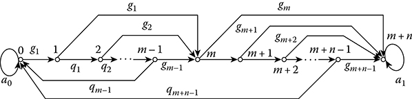
FIGURE 4.8 False target range track detection algorithm by criterion “2/m + 1/n.”
ViI=V1i3,
where
V1=8vrmaxvβmaxvεmaxδrδβδεT30.(4.29)
The volume of gates at the second stage of target range track detection is determined by
VIIj=8k3σΣjrσΣjβσΣjεδrδβδε,(4.30)
where k ≈ 3 is the coefficient of gate dimension increasing in comparison with magnitudes of the total mean square deviations of target pips from the gate center. There is a need to emphasize that the gate with definite dimensions corresponds to each graph state from 1 to (m + n − 1).
To define the probability of false target range track detection, first of all, there is a need to define the conditional probability p1 of event that a random point starting its movement from state a1 can reach anywhere in state am+n and will stay at this state. This probability can be defined as solving a system of linear equations that can be found based on the graph presented in Figure 4.8:
{p1=qf1p2+gf1pm,p2=qf2p3+gf2pm,……………………,pm−1=gfm−1pm,pm=qfmpm+1+gfm,pm+1=qfm+1pm+2+qfm+1,…………………,pm+n−1=gfm+n−1,(4.31)
where gfi i = 1,2,…, m − 1, is the probability of appearance of the false target pips within the gates with primary lock-in:
qfi=1−gfi;(4.32a)
gfj = j = m, m + 1, …, m + n − 1, is the probability of appearance of the false target pips within the confirmation gates:
qfj=1−gfj.(4.32b)
Solution of the linear equation system for arbitrary m and n is given by
p1=(1−m−1∏i=1qfi)(1−m+n−1∏j=mqfj).(4.33)
Equation 4.33 allows us to define the conditional probability of detection of the false target range track. This probability can be presented in the following form:
p1=pbeg×pconf,(4.34)
where
pbeg is the conditional probability of new target range track beginning
pconf is the conditional probability of confirmation of new target range track beginning
The unconditional probability of detection of the false target range track is given by
Pftr=P1×p1,(4.35)
where P1 is the probability of a single false target pip appearance that can be considered as the new target range track beginning. If we consider a general case for the confirmation criterion “l/m,” it is impossible to obtain the probability pconf in a general form. For this reason, these criteria are analyzed individually.
Filtering ability of the target range track detection algorithm can be characterized by average number ˉNftr
ˉNftr=p1×ˉN1,(4.36)
where ˉN1
The number of individual target pips becoming initial points of newly obtained false target range tracks after the (r+ 1)th radar antenna scanning can be determined by the following formula:
N1(r+1)=Nf(r+1)−m+n−1∑j=1gfjNj(r),(4.37)
where
j = 1,2,…, m + n − 1
Nf(r + 1) is the number of false target pips that is reprocessed by computer subsystem within the (r + 1)th radar antenna scanning
gfj is the probability of appearance of false target pips within the gate of volume Vj; the number of such gates is equal to m + n − 1
Nj(r) is the number of gates with the volume Vj formed within the rth radar antenna scanning ∑m+n−1j=1gfjNj(r)
∑m+n−1j=1gfjNj(r) is the number of false target pips of the current radar antenna scanning appearing within the gates of all false target range tracks that are under detection process, but a condition of no overlapping gates must be satisfied
In turn,
Nj(r)=r∑i=0N1(i)P(r−i)1j,(4.38)
where
N1(i) is the number of initial points of the false target range tracks formed within the ith radar antenna scanning
P(r−i)1j
P(r−i)1j is the probability of system transition (see Figure 4.8) from the initial state a1 to the state aj for (r – j) steps
Using (4.37) we should take into consideration that
N1(0)=Nf(0)andP(0)1j={1atj=1,0atj>1.(4.39)
Introduce a new variable s = r − i in (4.39) that corresponds to the relocation of the origin at the instant of finishing the ith radar antenna scanning. The variable s represents the number of steps (the radar antenna scanning) necessary for the transition of target range track detection algorithm graph from the initial state a1 to the state aj. In the case of target range track detection algorithm with criterion “2/m + 1/n,” the maximum value of s corresponds to the maximum number of steps needed for transition from the initial state a1 to the state am+n−1 and is equal to
smax=m+n−2.(4.40)
It is easy to verify this condition if we can define the longest branch in the algorithm graph presented in Figure 4.8. Taking into consideration all transformations discussed earlier, we obtain
Nj(r)=m+n−2∑s=0N1(r−s)P(s)1j.(4.41)
Analyzing (4.41), we see that the terms for which the following condition P(s)1j≠0
P(s)11={1ats=0,0ats>0,P(s)12=P(s−1)11qf1,P(s)13=P(s−1)12qf2,………………,P(s)1m=P(s−1)11gf1+P(s−1)12gf2+…+P(s−1)1,m−1gfm−1=m−1∑i=1P(s−1)1iqfi,P(s)1,m−1=P(s−1)1,mqfm,………………,P(s)1,m+n−1=P(s−1)1,m+n−2qfm+2−2.(4.42)
Taking into consideration (4.41), we can present (4.37) in the following form:
N1(r+1)=Nf(r+1)−m+n−1∑j=1gfjm+n−2∑s=0N1(r−s)P(s)1j.(4.43)
In steady working state (r → ∞) we can assume
N1(r+1)=N1(r)=N1(r−1)=…=N1[r−(m+n−2)]=ˉN1.(4.44)
Then we obtain
Nf(r+1)=Nf(r)=…=Nf[r−(m+n−2)]=ˉNf;(4.45)
ˉN1=ˉNf−ˉN1m+n−1∑j=1gfjm+n−2∑s=0P(s)1j(4.46)
and, finally we obtain
ˉN1=ˉNf1+∑m+n−1j=1gfj∑m+n−2s=0P(s)1j.(4.47)
Formula (4.47) combined with linear equation system (4.42) allows us to determine the average number of starting points of false target range tracks per radar antenna scanning in the steady working state of radar system. Knowing ˉN1
ˉN1=ˉNf1+∑m+v−1j=1gfj∑m+n−2s=0P(s)1j.(4.48)
where v is the number defined from target range track detection algorithm graph.
Results of determination of the average number ˉNftr
Filtering ability of target range track detection algorithms realizing the criterion “2/m + l/n” increases with a decrease in m and n and with an increase in l.
Incrementing l on unit leads to a great increase in the filtering ability, in comparison with a corresponding decrease in m and n.
These features must be taken into consideration while choosing the target range track detection algorithm implemented in practice. If the computer subsystem of a CRS has limitations in the number of false target range tracks that are to be tracked, then joint choice of the average number ˉNftr
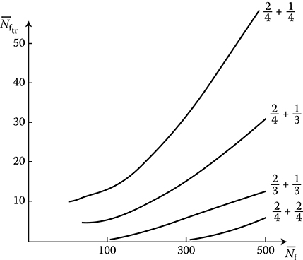
FIGURE 4.9 Comparison of filtering ability.
While designing the reprocessing of the CRS computer subsystem, there is a need to have information about the average number of false target range tracks that are under detection in the steady working state of a CRS. Denote this number by Ndftr
Ndftr=m+v−1∑j=1ˉNj,(4.49)
where in accordance with (4.41) in the steady working state of the CRS we have
ˉNj=ˉN1m+n−2∑s=0P(s)1j.(4.50)
Substituting (4.49) in (4.50), we obtain
Ndftr=ˉN1m+v−1∑j=1m+n−2∑s=0P(s)1j,(4.51)
or taking into consideration (4.48), we obtain finally
Ndftr=ˉNf∑m+v−1j=1∑m+n−2s=0P(s)1j1+∑m+v−1j=1gfj∑m+n−2s=0P(s)1j.(4.52)
4.2.3 STATISTICAL ANALYSIS OF “2/m + 1/n” ALGORITHMS UNDER TRUE TARGET RANGE TRACK DETECTION
First, we consider the simplest algorithm realizing the criterion “2/m + 1/n.” Functioning of the true target range track detection algorithm by the criterion “2/m + 1/n” is explained using Figure 4.10. A great feature of the true target range track detection algorithm graph in comparison with the false target range track detection algorithm graph shown in Figure 4.8 is the presence of nonzero probabilities of transitions to the initial state a0 from any intermediate state aj, where j = 1, 2,…, m + n − 1. The probability of replacement from the intermediate state ai, where i = 1, 2,…, m − 1, to the initial state a0 is equal to the probability of two simultaneous events. The first event is that the true target pip does not appear in the corresponding gate with primary lock-in; the second event is that at least one false target pip appears within the gate with primary lock-in, that is,
pi0(r)=[1−ptr(r)]gfi,(4.53)
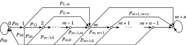
FIGURE 4.10 True target track detection algorithm graph by criterion “2/m + 1/n.”
where
ptr(r) is the probability of true target pip detection in the course of the rth radar antenna scanning, which is independent of the gate volume Vi
gfi is the probability of detection at least one false target pip within the gate volume Vi
The probability of replacement to the initial state a0 from any intermediate state aj, where j = m, m + 1,…, m + n − 1, is equal to the sum of the probabilities of two inconsistent events Ar and Br:
Pi0(r)=Pj(Ar)+Pj(Br),(4.54)
where j = m, m + 1,…, m + n − 1;
Pj(Ar)=[1−ptr(r)]gfi;(4.55)
Pj(Br)=ptr(r)gfi[1−Pind(Vj)];(4.56)
Pind(Vj) is the probability of indication of true target pip among false target pips within the gate volume Vi.
Thus, based on the general principles of target range track detection algorithm functioning and taking into consideration (4.53) through (4.56), we can define the probabilities of transitions pij(r) for the algorithm graph shown in Figure 4.10 or elements of corresponding transient probability matrix. These probabilities are determined as follows:
{p00(r)=1−ptr(r);p01(r)=ptr(r);p10(r)=gfi[1−ptr(r)];p12(r)=(1−gfi)[1−ptr(r)];p1m(r)=ptr(r);……………………pm−1,0(r)=1−ptr(r);pm−1,m(r)=ptr(r);……………………pm0(r)=[1−ptr(r)]gfm+ptr(r)gfm[1−Pind(Vm)];pm,m+1(r)=[1−ptr(r)](1−gfi);pm,m+n(r)=ptr(r)(1−gfi)+ptr(r)gfmPind(Vm);……………………pm+n−1,0(r)=[1−ptr(r)]gfm+n−1+ptr(r)gfm+n−1[1−Pind(Vm+n−1)];pm+n−l,m+n(r)=ptr(r)(1−gfm+n−1)+ptr(r)gfm+n−1Pind(Vm+n−1);pm+n,m+n(r)=1.(4.57)
We would like to stress again that the probability of the target return signal detection for the formulas of probabilities of transition given by (4.57) is determined by the following [14–17]:
P(r)=‖P0(r)P1(r)…Pm+n(r)‖=P(r−1)∏(r),(4.58)
where
P(r − 1) is the row vector of probabilities of states at the previous (r − 1)th radar antenna scanning step
π(r) is the matrix of transient probabilities at the rth radar antenna scanning step
In accordance with (4.58) and taking into consideration (4.57), these equations define the elements of the transient probability matrix π(r), and the system of recurrent equations to define components of the vector P(r) can be presented in the following form:
{P0(r)=P0(r−1)p00(r)+P1(r−1)p10(r)+…+Pm+n−1(r)pm+n−1,0(r)=m+n−1∑j=1Pj(r−1)pj0(r);P1(r)=P0(r−1)p01(r);…………………………Pm(r)=P1(r−1)p1,m(r)+P2(r−1)p2,m(r)+…+Pm−1(r−1)pm−1,m(r)=m+n−1∑j=1Pj(r−1)pj,m(r);Pm+1(r)=Pm(r−1)pm,m+1(r);…………………………Pm+n(r)=m+n−1∑j=mPj(r−1)pj,m−n(r)+Pm+n(r−1)=Ptrue(r).(4.59)
The last line in (4.59) defines the total probability of true target range track detection at the rth radar antenna scanning increasing from scanning to scanning.
If we consider a general case of the criterion “2/m+ 1/n,” it is impossible to obtain the formula for increasing the probability of true target range track detection at an arbitrary value of l if l > 1. There is a need to carry out analysis for each individual target range track detection algorithm [18-20]. To compare various criteria of the type “2/m + l/n” used under the true target range track detection, the probability of detection as a function of normalized target range dr/dmax determined based on discussed procedure is presented in Figure 4.11. In accordance with adopted notations, dmax is the maximal horizontal radar range; dr is the current horizontal radar range:
dr=dmax−rΔd(Tsc)(4.60)
where d(Tsc) is the variation of radar range coordinate within the limits of the radar antenna scanning period Tsc. The probability of target detection at the rth radar antenna scanning is determined by the formula
Ptg(r)=exp[−0.68d4rd4max].(4.61)
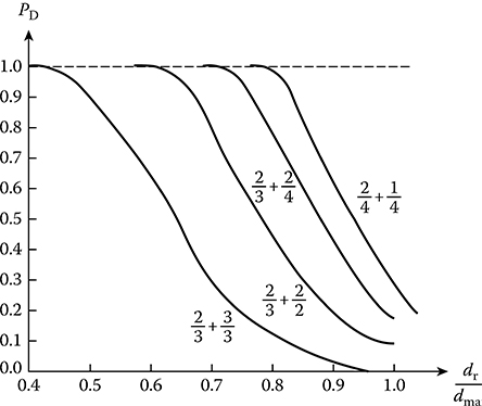
FIGURE 4.11 Probabilities of true target range track detection for various criteria “2/m + l/n.”
The probability of true indication of target pips within confirmation gates is considered constant and equal to Pind = 0.95. Density of false target pips per unit volume of radar antenna scanning area is equal to 10−4.
Analysis and comparison of performance shown in Figure 4.11 allow us to conclude that it is worthwhile to employ the criterion “2/m + 1/n” based on the viewpoint of decreasing the number of steps under detection of true target range track. In doing so, small deviations in m and n do not lead to great changes in the number of steps to ensure the probability of true target range track detection close to the unit. The probability of true target range track detection equal to 0.95 using the discussed criteria is obtained for target range corresponding to 0.75 of the maximal radar system range. Implementation of confirmation criteria “l/n” (l > 1) leads to the prolongation of time to detect the true target range tracks.
4.3 Target Range Tracking Using Surveillance Radar Data
If the earlier-given criterion of target detection is satisfied, the signal processing of the target return signal is finished at the stage of target range track detection. After that initial parameters of detected target range track are determined, and this target range track will be under autotracking. Henceforth, the target autotracking is considered as automatic target range track prolongation of target moving and accurate definition of prolongated target range track parameters. Thus, the terms “target autotracking” and “autotracking” (or “tracking”) must be understood in the same sense. Furthermore, we prefer to use the term “target range autotracking” or “target autotracking.”
4.3.1 TARGET RANGE AUTOTRACKING ALGORITHM
In the course of each target range tracking, two main problems are solved: gating and selection of newly obtained target pips for prolongation of target range track, estimation of target range track parameters, and definition of variation of these parameters as a function of time. In principle, solution of both problems can be realized employing the same detection algorithm. In this case, a required quality of the solved target range track estimation parameter problem must be in agreement with the customer. However, there is such a target range autotracking system in which the autotracking algorithm hunts only for target range track. To achieve a high-quality estimate of the target range track parameters, the individual target range track detection algorithm must be designed. Henceforth, we term this detection algorithm as target range track detection algorithm computations. Expediency to design the target range track detection algorithm computations arises from the following principles:
Operations of estimation and extrapolation of target range track parameters must be carried out in the radar coordinate system to ensure the continuity of target range autotracking as soon as the input information is changed. There are no hard restrictions over the accuracy of these operations that allow us to use simple formulas for computations based on a hypothesis about straight-line target moving.
Computations of target range track parameters must be carried out using very precise formulas, taking into consideration all available information about the target movement character (air or cosmic target, maneuvering or nonmaneuvering target, etc.) in the interests of customers. In doing so, the parameter output can be presented in other coordinate systems that are different from a radar coordinate system, for example, the Cartesian coordinate system with the center at the point gathering information. Moreover, to estimate the necessary target range track parameters, for example, a course and velocity vector modulus under aircraft autotracking, the parameters that are not associated with the target range autotracking can be selected based on the needs of the customer or with the purpose of matching them with other detection algorithms of a CRS.
The customer is interested, first of all, in target information that is very important for a CRS, for example, the information about the type and number of aircraft following for landing stored into the automatic control system of airport. The exact target range track parameters must be determined using just these targets. Naturally, not all detected targets within the radar antenna scanning area are important and some of them are not interested in a CRS, for example, recessive targets, transiting targets, and so on. Consequently, an estimation of target range track parameters with high accuracy is necessary only for a very small part of autotracked targets. In the considered case, definition of individual target range autotracking algorithm allows us to reduce requirements to computer system speed.

FIGURE 4.12 Block diagram of the target range tracking algorithm.
Logical block diagram of the target range tracking algorithm is presented in Figure 4.12 based on the statements discussed earlier. Block 1 solves the problem of selection and indication of target pip to continue the target range tracking. The gating algorithm and indication of target pips within the gate is designed in accordance with theoretical assumptions discussed in Section 4.1. The indicated target pip is given the number of tracked target range trajectory and it is processed by the block of target range track computations (the block 6). Simultaneously, the newly obtained target pip is used to estimate the parameters of target range track and to extrapolate the target coordinate for the next radar antenna scanning process, that is, to prepare a new gating cycle and indication. For this purpose the following operations are carried out:
Estimation of target range track parameters under simplest conditions of target moving and coordinate measurement errors (the block 2).
Determination of the extrapolated coordinates for the next radar antenna scanning (the block 3). Extrapolation is carried out by linear law.
Determination of gate dimensions (the block 4). At the same time, the accurate characteristics of measured and extrapolated coordinates and information about a target pip miss within the gate are used.
When the newly obtained target pip is absent, we check the criterion of cancellation of the target range tracking with the purpose to prolong the target range track (the block 5). If the cancellation criterion is satisfied, the target range tracking is stopped and the previous information about this target range track is removed. When the cancellation criterion is not satisfied, the coordinates of extrapolated point are used as the coordinates of newly obtained target pip and the computation process is repeated.
In general, in addition to the presence of the target pips within the gate that prolongs the target range track, we should take into consideration a set of other factors such as the target importance; target maneuverability, that is, to change a target range track during the fight; current target coordinates; direction of target moving; and length of target visibility within radar antenna scanning area and so on to make a decision about the target range tracking cancellation. However, a recordkeeping of these factors is very difficult and is not accessible forever owing to limitations in the speed of a computer system. For this reason, the main criterion while making a decision about the target range tracking cancellation is the appearance of some threshold series kth of target pip misses within tracking gates. This criterion of cancellation of the target range tracking does not take into consideration individual peculiarities of each target range track and does not use information about accumulated accuracy level at the instant of appearance of the target pip miss series. A single advantage of this criterion is its simplicity.
While choosing kth there is a need to proceed from the following assumptions. The greater is the value of kth, the smaller is the probability to make a false decision about cancellation of the true target range track. On the other hand, with an increase in the value of kth, the number of false target range tracking and its average length is increased. Because of this, while choosing kth there is a need to take into consideration the statistical characteristics of true target pip misses (no detections). The final choice of the value of kth is usually carried out in the course of testing the signal processing subsystem.
Taking into consideration the criterion of target range track cancellation by kth misses one after another, the target range tracking process is described by the graph with random transitions (see Figure 4.13). The character of states and transitions of this graph allows us to select the following modes of the target range tracking:
The mode of stable target range tracking characterizing that the graph is at the initial state am+n. For the first time, this state is obtained when the criterion of target range track detection is satisfied.
The mode of unstable target range tracking corresponding to one of the intermediate states of the graph, namely, aj, where j = m + n − 1,…, m + n + kth − 1.
The mode of target range tracking cancellation indicating the fact that the number of target pip misses one after another could reach the threshold level k = kth and the graph has been passed into the state am+n+kth.
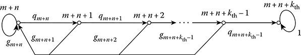
FIGURE 4.13 Target range tracking graph with random transitions.
In this case, the target range tracking algorithm graph is analogous to the graph of binary quantized target return pulse train latching algorithm [21–23]. For this reason, a procedure of analysis of these algorithms is the same.
Under statistical analysis of target range tracking algorithms, the main interest is the average time of false target range track observation and the average number of false target range tracking in the steady working state, which is associated with the average time of false target range track observation. Moreover, it is very interesting to define the probability of true target range tracking cancellation at the given probability of target pip detection within the gate. Let us define a function between the average number of false target range tracking for each radar antenna scanning period and the average number of false target range tracks in the steady working state. For this purpose, first of all, there is a need to define the probability to stop exactly the false target range tracking process at the μth step (the radar antenna scanning period) after starting the false target range tracking at the instant μ = 0. In the case of cancellation criterion by kth misses one after another, the probability to stop exactly the false target range tracking process at the μth step (the radar antenna scanning period) is equal to the probability of graph transition from the state am+n to the state am+n+kth in the course of μ steps (see Figure 4.13):
Pcan(μ)=Pm+n+kth(μ).(4.62)
To determine the probability Pm+n+kth (µ), we can use the following recurrent formulas:
{Pm+n(0)=1,Pm+n(μ)=m+n+ktr−1∑j=m+nPj(μ−1)gfi,Pm+n+1(μ)=Pm+n(μ−1)gfm+n,…………………………………Pm+n+kth(μ)=Pm+n+kth−1(μ−1)gfm+n+kth−1.(4.63)
The average length of the false target range tracks expressed as the number of radar antenna scanning periods is defined in the following form:
ˉμ=∞∑μ=kthμPm+n+kth(μ).(4.64)
Furthermore, when we know the average number of the false target range tracks, the average number of the false target range tracks being under tracking is determined by
ˉNtrackingftrack=ˉNftrackˉμ.(4.65)
The average number of the false target range tracks being under tracking is taken into account under the definition of computer subsystem cost and speed.
4.3.2 UNITED ALGORITHM OF DETECTION AND TARGET RANGE TRACKING
Until now, we have assumed that the target range track detection and tracking algorithms are realized individually, that is, by the individual computer subsystems. In practice, for the majority of cases, it is very convenient to employ such structure of signal reprocessing subsystems where the target range track detection and tracking algorithms are united and presented in the form of a single algorithm of target range track detection and tracking, and realization of this united algorithm is carried out by individual computer subsystem. Henceforth, we consider this version of structure of signal reprocessing subsystem.
If the criterion of beginning the target range track “2/m,” the criterion of confirmation of the target range track “l/n,” and the criterion of cancellation of target range tracking, for example, the criterion using kth misses one after another, are given, then the united criterion of detection and tracking of the target range track can be written in the symbolic notation “2/m + l/n - kth.” The graph of the united algorithm under detection and tracking of target range track by criterion “2/m + l/n - kth” is shown in Figure 4.14. This graph allows us to analyze the processes of detection and tracking of target range tracks as a whole instead of analysis by parts discussed earlier. Based on this graph, we can present an accurate formula defining the initial points of false target range tracks forming in the course of the steady working state (see (4.48)).
In the united algorithm realizing the criterion “2/m + l/n − kth,” the number of gates is equal to m + v + kth − 1. Because of this, the upper limit of summation by j in (4.48) will be jmax = m + v + kth − 1. The upper limit of summation by s will be defined as smax → ∞ since the number of steps under transition from the state a1 to the state am+n+kth − 1 will be arbitrary large.
Thus, in the united algorithm case, the number of false target pips obtained at the initial points of new target range tracks is determined by the following formula:
ˉN'1=ˉNf1+∑m+v+kth−1j=1gfj∑∞s=0P(s)1j.(4.66)
If the criterion of confirmation takes the form “1/n,” we obtain v = n. The average number of false target range tracks for tracking is determined as
N′ftr=ˉN′1p1,(4.67)
which is less than that of individual realization since the number of initial points is decreased. The number of false target range tracks being under tracking will also decrease correspondingly.
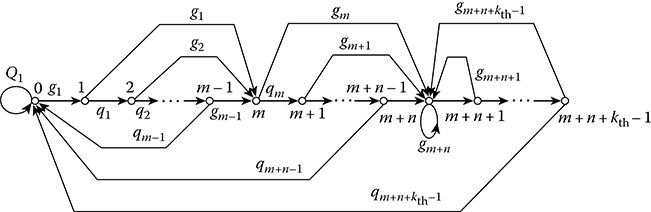
FIGURE 4.14 Graph of the united algorithm under detection and tracking of target range track by criterion “2/m + l/n − kth.”
4.4 Summary and Discussion
Target range tracking is accomplished by continuously measuring the time delay between the transmission of an RF pulse and the echo signal returned from the target, and converting the roundtrip delay into units of distance. The target range measurement may also be performed with continuous wave (CW) radar systems using the frequency-modulated continuous wave (FM-CW) that is typically a linear-ramp FM. The target range is determined by the range-related frequency difference between the echo-frequency ramp and the frequency of the ramp being transmitted. The first function of the target range tracker is acquisition of a desired target. Although this is not a tracking operation, it is a necessary first step before the target range tracking or target angle tracking (the azimuth tracking) may take place in a typical radar system. The range-tracking portion of the radar has the advantage of seeing all targets within the beam from close range out to the maximum range of the radar. It typically breaks this range into small increments, each of which may be simultaneously examined for the presence of a target. When beam scanning is necessary, the target range tracker examines the increments simultaneously for short periods, such as 0.1 s, makes its decision about the presence of a target, and allows the beam to move to a new location if a “no” target is present.
Once a target is acquired in range, it is desirable to follow it in the range coordinate to provide distance information or slant range to the target. Appropriate timing pulses provide a target range gating so the angle-tracking circuits and automatic gain control (AGC) circuits look at only the short target range interval, or time interval, when the desired echo pulse is expected. The target range tracking operation is performed by closed-loop tracking similar to the azimuth tracker. Error in centering the range gate on the target echo pulse is sensed, error voltages are generated, and circuitry is provided to respond to the error voltage by causing the gate to move in a direction to recenter on the target echo pulse. Automatic target range tracking can generally be divided into five steps: (a) radar detection acceptance, accepting or rejecting detections for insertion into the tracking process—the purpose of this step is to control false track rates; (b) association of accepted detections with existing tracks; (c) updating the existing tracks with associated detections; (d) new track formation using unassociated detections; and (e) radar scheduling and control.
In the course of target range track detection the following operations are carried out: (a) gating and selection of target pip within the gate, (b) checking the detection criterion, and (c) estimation and extrapolation of target range track parameters. Target range tracking is sequential from measuring to measuring procedure of newly obtained target pip binding to target range track and accurate target range track determination. Under target range autotracking, the following operations are carried out: (a) accurate definition of target range track parameters in the course of newly obtained target pip binding, (b) extrapolation of target range track parameters for the next radar antenna scanning, (c) range gating of possible newly obtained target pip positions, and (d) selection of the definite target pip within the gate if there are several target pips within the gate area. When there are several target pips within the tracking gate, we expand the target range track binding for each target pip. When the target pip is absent within the tracking gate, the target range track is prolonged by the corresponding extrapolated point, but the next gate is increased in area to take into consideration the errors increasing in the course of extrapolation. If there are no target pips during k radar antennas scanning following one after another, the target range tracking is canceled. Thus, at various stages of target range track detection and target range tracking, we carry out the same operations in reality: (a) radar antenna scanning area gating, (b) selection and identification of target pips within the gate, and (c) filtering and extrapolation of target range track parameters.
While the CRS computer subsystem processes a high number of targets in real time, computation of dimensions and orientation of parallelepiped gate sides is very cumbersome. In this case, there is a need to use a simple version of gating, which is described as follows. The simplest gate shape is chosen for definition in that coordinate system, wherein radar information is processed. In the case of spherical coordinate system, the simplest gate is given by a linear dimension in target range Δrgate and by two angular dimensions, namely, by the azimuth Δβgatte and elevation Δεgate (see Figure 4.4). These dimensions can be set in advance, based on the maximal magnitudes of random and dynamic errors while processing all target range tracks. In short, in this case, the gate dimensions are chosen so that the ellipsoid of all possible (under all directions of target moving and fight) total deviations of true target pips from corresponding extrapolated points will be easily fit and rotated in any direction inside the gate. This is the crudest technique of gating. We note that all procedures to choose dimensions of 3D gate can be used in full under gating in plane for binding newly obtained target pips in 2D radar systems.
The quality of target pip indication process can be evaluated by the probability of correct indication; in other words, the probability of event that the true target pip will be indicated to prolong the target range track in the next radar antennas scanning. The problem of definition of the probability of correct indication can be solved analytically if we assume that a presence of false target pips within the gate is only caused by a stimulus of the noise and interference and these target pips are uniformly distributed within the limits of radar antenna scanning area. Under indication within 2D rectangle gate circumscribed around the ellipse with the parameter equal λmax ≥ 3, the probability of correct indication is determined by
Pind=11+2πρsσησξ,
where
ρs is the density of false target pips per unit square of gate
ση and σξ are the mean square deviations of true target pips from the gate center along the axes η and ξ
In the case of target pip indication in 3D gate that can be presented in the form of parallelogram circumscribed around the total error ellipsoid, the probability of correct indication is determined by
Pind≈1−21.33πσησξσζρv√2π,
where ρV is a density of false target pips per unit volume of gate.
We can note that in addition to target pip deviations from the gate center, the weight features of target pips formed in the course of signal preprocessing, as some analog of SNR, can be used to indicate the target pips. In the simplest case of binary quantized target return pulse train, we can use the number of train pulses or train bandwidth to generate the target pip weight features. Weight features of target pips can be used under target range track indication jointly with features of target pip deviations from the gate center or independently. One of the possible ways to use the target pip weight features jointly with the target pip deviations from the gate center is as follows. All target pips within the gate are divided with weight v1 and with weight v0 depending on whether the target return pulse train bandwidth exceeds the earlier-given threshold value or not, which in turn depends on target range magnitude. If there are target pips with weight v1 we indicate the target pip that is nearest to the gate center as the true target pip from the observed target pip group. If there are no target pips with weight v1, we indicate the target pip with weight v0 that is nearest to the gate center as the true target pip. If we can characterize the target pip weight by the number of pulses in the target return pulse train, then we are able to indicate the target range track by the maximum number of pulses in the target return pulse train. In this case, features of target pip deviations from the gate center are only used under equality of weights of several target pips.
Under a hard noise environment, several gates formed around extrapolated points of prolonged target range tracks will be overlapped. Moreover, false and newly obtained target pips will appear within the gates. In this case, the problem of newly obtained target pip distribution and binding to target range tracking becomes more complex. In addition, the problem of fixing the beginning of a new target range track arises. First of all, this complication is associated with the necessity to use a joint target pip binding to target range track after getting newly obtained target pips liable to binding or, in other words, if these newly obtained target pips are within overlapping gates. There is a need to generate all possible ways or hypotheses for target pip binding and choose the most plausible version. After the determination of probabilities of events that the target pips belong to the existing target range tracks, new target range tracks, and false target range tracks, we are able to determine the probabilities of all versions of the target pip binding and to choose the version with the highest probability as a true version. Solution of this problem is very tedious even for the case that is considered the simplest. This problem can be simplified if the following practical rules are followed: (a) each target range track must be attached by the target pip, and (b) if the target pip is not associated to the given-before target range track, then a new target range track must be started independently of the probability of event that this target pip belongs to the new target range track or false target range track; in this case, we should compare only versions when there are target pip bindings for each target range track.
The process of target range track detection is divided into two stages: (a) the first stage is the target range track detection by criterion “2/m” and (b) the second stage is the confirmation of beginning the target range track, that is, the final target range track detection by criterionm “l/n.” In particular cases of the second stage, the target range track detection may be absent. Algorithm of the target range track detection by criterion “2/m” jointly with the confirmation algorithm or final target range track detection by criterion “l/n” forms a united target range track detection algorithm by criterion “2/m + l/n.” The main computer subsystem operations carried out under target range track detection are as follows: (a) evaluation of target velocity under moving, (b) extrapolation of coordinates, and (c) gating the target pips. Target range track detection quality can be evaluated by the following characteristics: (a) the probability of detection of true target range track, (b) average number of false target range tracking per unit time, and (c) speed of computer systems used to realize the target range track detection algorithm.
Results of determination of the average number ˉNftr
Analysis and comparison of performance shown in Figure 4.11 allow us to conclude that it is worthwhile to employ the criterion “2/m + 1/n” based on the viewpoint of decreasing the number of steps under detection of true target range track. In doing so, small deviations in m and n do not lead to great changes in the number of steps to ensure the probability of true target range track detection close to the unit. The probability of true target range track detection equal to 0.95 using the discussed criteria is obtained for target range corresponding to 0.75 of the maximum radar system range. Implementation of confirmation criteria “l/n” (l > 1) leads to the prolongation of time to detect the true target range tracks.
In the course of each target range tracking, two main problems are solved: gating and selection of newly obtained target pips for the prolongation of target range track, estimation of target range track parameters, and definition of variations in these parameters as a function of time. In principle, solutions to both problems can be obtained by employing the same detection algorithm. In this case, the required quality of a solved target range track estimation parameter problem must be in agreement with the customer requirements. However, there is a version of target range autotracking system in which the autotracking algorithm hunts only for target range track. To achieve a high-quality estimate of the target range track parameters, the individual target range track detection algorithm must be designed.
In general, in addition to the presence of the target pips within the gate to prolong the target range track, we should take into consideration a set of other factors such as the target importance; target maneuverability, that is, to change a target range track during the fight; current target coordinates; direction of target moving; and length of target visibility within radar antenna scanning area and so on to make a decision about the target range tracking cancellation. However, a recordkeeping of these factors is very difficult and is not accessible forever owing to limitations in the computer system speed. For this reason, the main criterion for decision about the target range tracking cancellation is the appearance of some threshold series kth of target pip misses within tracking gates. This criterion of cancellation of the target range tracking does not take into consideration individual peculiarities of each target range track and does not use information about accumulated accuracy level at the instant of appearance of the target pip miss series. A single advantage of this criterion is its simplicity.
In practice, in the majority of cases, it is very convenient to employ a structure of signal reprocessing subsystems in which the target range track detection and tracking algorithms are united and presented in the form of a single algorithm of target range track detection and tracking, and realization of this united algorithm is carried out by the individual computer subsystem. If the criterion of beginning the target range track “2/m,” the criterion of confirmation of the target range track “l/n,” and the criterion of cancellation of target range tracking, for example, the criterion using kth misses one after another are given, then the united criterion of detection and tracking of the target range track can be written in the following symbolic notation “2/m + l/n − kth”. The graph of the united algorithm under detection and tracking of target range track by criterion “2/m + l/n − kth” is shown in Figure 4.14. It allows us to analyze the processes of detection and tracking of target range tracks as a whole instead of analysis by parts, as discussed previously. On the basis of this graph, we can present an accurate formula that defines the initial points of false target range tracks forming in the course of the steady working state (see (4.48)).
References
1. Sherman, S.M. 1986. Monopulse Principles and Techniques. Norwood, MA: Artech House, Inc.
2. Trunk, G.V. 1978. Range resolution of targets using automatic detectors. IEEE Transactions on Aerospace and Electronic Systems, 14(9): 750–755.
3. Trunk, G.V. 1984. Range resolution of targets. IEEE Transactions on Aerospace and Electronic Systems, 20(11): 789–797.
4. Trunk, G.V. and M. Kim. 1994. Ambiguity resolution of multiple targets using pulse Doppler waveforms. IEEE Transactions on Aerospace and Electronic Systems, 30(10): 1130–1137.
5. Bath, W.G., Biddison, L.A., Haase, S.F., and E.C. Wetzlat. 1982. False alarm control in automated radar surveillance system, in IEE International Radar Conference, London, U.K., pp. 71–75.
6. Stuckey, W.D. 1992. Activity control principles for automatic tracking algorithms, in IEEE Radar’92 Conference, October 12–13, Birghton, U.K., pp. 86–89.
7. Leonov, A.I. and K.I. Formichev. 1986. Monopulse Radar Norwood, MA: Artech House, Inc.
8. Barton, D.K. 1988. Modern Radar System Analysis. Norwood, MA: Artech House, Inc.
9. Bar-Shalom, Y. and T. Forthmann. 1988. Tracking ad Data Association. Orlando, FL: Academic Press.
10. Mookerjee, P. and F. Reifer. 2004. Reduced state estimator for system with parametric inputs. IEEE Transactions on Aerospace and Electronic Systems, 40(2): 446–461.
11. Leung, H., Hu, Z., and. M. Blanchette. 1999. Evaluation of multiple radar target trackers in stressful environments. IEEE Transactions on Aerospace and Electronic Systems, 35(12): 663–674.
12. Blair, W.D. and Y. Bar-Shalom. 1996. Tracking maneuvering targets with multiple sensors: Does more data always mean better estimates? IEEE Transactions on Aerospace and Electronic Systems, 32(1): 450–456.
13. Simson, G.W. 1998. Introduction to Airborne Radar. 2nd edn. Mendham, NJ: SciTech Publishing.
14. Gumming, I.G. and F.N. Wong. 2005. Digital Processing on Synthetic Aperture Radar Data. Norwood, MA: Artech House, Inc.
15. Guerci, J.R. 2003. Space-Time Adaptive Processing for Radar. Norwood, MA: Artech House, Inc.
16. Levanon, N. and E. Mozeson. 2004. Radar Signals. New York: John Wiley & Sons, Inc.
17. Sullivan, R.J. 2000. Microwave Radar: Imaging and Advanced Concepts. Boston, MA: Artech House, Inc.
18. Peebles, P.Z. Jr. 1998. Radar Principles. New York: John Wiley & Sons, Inc.
19. Hayes, M.H. 1996. Statistical Digital Signal Processing and Modeling. New York: John Wiley & Sons, Inc.
20. Billingsley, J.B. 2001. Radar Clutter. New York: John Wiley & Sons, Inc.
21. Blackman, S. and. R. Popoli. 1999. Design and Analysis of Modern Tracking Systems. Boston, MA: Artech House, Inc.
22. Cooperman, R. 2002. Tactical ballistic missile tracking using the interacting multiple model algorithm, in Proceedings of the Fifth International Conference on Information Fusion, July 8–11, Vol. 2, Annapolis, Maryland, pp. 824–831.
23. Pisacane, V.J. 2005. Fundamentals of Space Systems. 2nd edn. Oxford, U.K.: Oxford University Press.