Chapter 13 Estimation of Stochastic Process Variance

Search in book...
Toggle Font Controls
Create new playlist

Name your new playlist

Playlist description (optional)
Sign In

Email address

Password

Forgot Password?

or

Continue with Facebook

Continue with Google
Sign Up

Full Name

Email address

Confirm Email Address

Password

or

Continue with Facebook

Continue with Google

Let the stationary Gaussian stochastic process ξ(t) with the correlation function

$R (t_{1}, t_{2}) = σ^{2} ℛ (t_{1}, t_{2}) (13.1)$

be observed at N equidistant discrete time instants t_i, i = 1, 2,…, N in such a way that

$t_{i + 1} - t_{j} = Δ = const . (13.2)$

Then, at the measurer input we have a set of samples x_i = x(t_i). Furthermore, we assume that the mathematical expectation of observed stochastic process is zero. Then, the conditional N-dimensional pdf of Gaussian stochastic process can be presented in the following form:

$p (x_{1}, x_{2}, ..., x_{N} | σ^{2}) = \frac{1}{{(2 π σ^{2})}^{N / 2} \sqrt{\det ‖ ℛ_{i j} ‖}} \exp {- \frac{1}{2 σ^{2}} {\sum^{}}_{i = 1, j = 1}^{N} x_{i} x_{j} C_{i j}} (13.3)$

where

det ‖ℛ_ij‖ is the determinant of matrix consisting of elements of the normalized correlation function ℛ(t_i, t_j) = ℛ_ij
C_ij are the elements of the matrix that is reciprocal to the matrix ‖ℛ‖

In doing so, the elements C_ij are defined from the equation that is analogous to (12.170)

${\sum^{}}_{l = 1}^{N} C_{i l} ℛ_{l j} = δ_{i j} . (13.4)$

The conditional multidimensional pdf (13.3) is the multidimensional likelihood function of the parameter σ². Solving the likelihood equation, we obtain the variance estimate

${Var}_{E} = \frac{1}{N} {\sum^{}}_{i = 1, j = 1}^{N} x_{i} x_{j} C_{i j} = \frac{1}{N} {\sum^{}}_{i = 1 x}^{i = 1} x_{i} v_{j}, (13.5)$

where

$v_{i} = {\sum^{}}_{j = 1}^{N} x_{j} C_{i j} . (13.6)$

The random variables v_i possess zero mean and are subjected to the Gaussian pdf. Prove that the random variables v_i are dependent on each other and are mutually independent of the samples x_p at p ≠ i. Actually,

$〈 v_{j} v_{q} 〉 = {\sum^{}}_{j = 1, p = 1}^{N} C_{i j} C_{q p} 〈 x_{j} x_{p} 〉 = σ^{2} {\sum^{}}_{j = 1}^{N} C_{i j} {\sum^{}}_{p = 1}^{N} C_{q p} ℛ_{j p} = σ^{2} {\sum^{}}_{j = 1}^{N} C_{i j} δ_{j q} = σ^{2} C_{i q}; (13.7)$

$〈 x_{p} v_{j} 〉 = {\sum^{}}_{j = 1}^{j = 1} C_{i j} 〈 x_{j} x_{p} 〉 = σ^{2} {\sum^{}}_{j = 1}^{N} C_{i j} ℛ_{j p} = σ^{2} δ_{i p}, (13.8)$

where σ² is the true variance of the stochastic process ξ(t).

Determine the statistical characteristics of variance estimate, namely, the mathematical expectation and variance. The mathematical expectation of variance estimate is given by

$E {{Var}_{E}} = \frac{1}{N} {\sum^{}}_{i = 1, j = 1}^{N} C_{i j} 〈 x_{j} x_{j} 〉 = σ^{2}, (13.9)$

that is, the variance estimate is unbiased.

The variance of variance estimate can be presented in the following form:

$Var {{Var}_{E}} = \frac{1}{N^{2}} {\sum^{}}_{i = 1, j = 1}^{N} {\sum^{}}_{p = 1, q = 1}^{N} 〈 x_{i} x_{j} x_{p} x_{q} 〉 C_{i j} C_{p q} - σ^{4} . (13.10)$

Determining the mixed fourth moment of the Gaussian random variable x

$〈 x_{i} x_{j} x_{p} x_{q} 〉 = σ^{4} [ℛ_{i j} ℛ_{p q} + ℛ_{i p} ℛ_{j q} + ℛ_{i q} ℛ_{j p}] (13.11)$

and substituting (13.11) into (13.10) and taking into consideration (13.4), we obtain

$Var {{Var}_{E}} = \frac{2 σ^{4}}{N} . (13.12)$

As we can see from (13.12), the variance of the optimal variance estimate is independent of the values of the normalized correlation function between the samples of observed stochastic process. This fact may lead to some results that are difficult to explain with the physical viewpoint or cannot be explained absolutely. Actually, increasing the number of samples within the limits of the finite small time interval, we can obtain the estimate of variance with the infinitely small estimate variance according to (13.12). Approaching the variance of optimal variance estimate of Gaussian stochastic process to zero is especially evident while passing from discrete to continuous observation of stochastic process. Considering

$N = {\sum^{}}_{i = 1}^{N} {\sum^{}}_{j = 1}^{N} C_{i j} ℛ_{i j} (13.13)$

and applying the limiting process to (13.5) from discrete observation to continuous one at T = const (Δ → 0, N → ∞), we obtain

${Var}_{E} = \frac{{\int^{}}_{0}^{T} {\int^{}}_{0}^{T} ϑ (t_{1}, t_{2}) x (t_{1}) x (t_{2}) d t_{1} d t_{2}}{{\int^{}}_{0}^{T} {\int^{}}_{0}^{T} ϑ (t_{1}, t_{2}) ℛ (t_{1}, t_{2}) d t_{1} d t_{2}}, (13.14)$

where the function ϑ(t₁, t₂), similar to (12.6), can be defined from the following equation:

${\int^{}}_{0}^{T} ϑ (t_{1}, t) ℛ (t_{1}, t_{2}) d t = ℛ (t_{2} - t_{1}) . (13.15)$

Determining the mathematical expectation of variance estimate, we can see that it is unbiased. The variance of the variance estimate can be presented in the following form:

$Var {{Var}_{E}} = \frac{2 σ^{4}}{{\int^{}}_{0}^{T} {\int^{}}_{0}^{T} ϑ (t_{1}, t_{2}) ℛ (t_{1}, t_{2}) d t_{1} d t_{2}} . (13.16)$

Since

$\lim_{τ \to t_{2}} {\int^{}}_{0}^{T} ϑ (t_{1}, t_{2}) ℛ (τ, t_{1}) d t_{1} = δ (0) \to \infty, (13.17)$

we can see from (13.16) that the variance of the optimal variance estimate of Gaussian stochastic process approaches symmetrical to zero for any value of the observation interval [0, T].

Analogous statement appears for a set of problems in statistical theory concerning optimal signal processing in high noise conditions. In particular, given the accurate measurement of the stochastic process variance, it is possible to detect weak signals in powerful noise within the limits of a short observation interval [0, T]. In line with this fact, in [1] it was assumed that for the purpose of resolving detection problems, including problems related to zero errors, we should reject the accurate knowledge of the correlation function of the observed stochastic processes or we need to reject the accurate measurement of realizations of the input stochastic process. Evidently, in practice these two factors work. However, depending on which errors are predominant in the analysis of errors, limitations arise due to insufficient knowledge about the correlation function or due to inaccurate measurement of realizations of the investigated stochastic process.

It is possible that errors caused by inaccurate measurement of the investigated stochastic process have a characteristic of the additional “white” noise with Gaussian pdf. In other words, we think that the additive stochastic process

$y (t) = x (t) + n (t) (13.18)$

comes in at the input of measurer instead of the realization x(t) of stochastic process ξ(t), where n(t) is the realization of additional “white” noise with the correlation function defined as R_n(τ) = 0.5 $N_{0}$ σ(τ) and $N_{0}$ ₀ is the one-sided power spectral density of the “white” noise.

To define the characteristics of the optimal variance estimate in signal processing in noise we use the results discussed in Section 15.3 for the case of the optimal estimate of arbitrary parameter of the correlation function R(τ, l) of the Gaussian stochastic process combined with other Gaussian stochastic processes with the known correlation function. As applied to a large observation interval compared to the correlation interval of the stochastic process and to the variance estimate (l ≡ σ²), the variance estimate, in the first approximation, is unbiased. The variance of optimal variance estimate of the correlation function parameter given by (15.152) can be simplified and presented in the following form:

$Var {\frac{{Var}_{E}}{σ^{2}}} = \frac{1}{{\frac{T}{4 π} {\int^{}}_{- \infty}^{\infty} \frac{S^{2} (ω) d ω}{{[σ^{2} S (ω) + 0.5 N_{0}]}^{2}}}^{2}}, (13.19)$

where S(ω) is the spectral power density of the stochastic process ξ(t) with unit variance.

To investigate the stochastic process possessing the power spectral density given by (12.19), the variance of the variance estimate in the first approximation is determined in the following form:

$Var {\frac{{Var}_{E}}{σ^{2}}} = \frac{4 σ^{2} \sqrt{α N_{0} σ^{2}}}{α T} . (13.20)$

Denote

$P_{n} = N_{0} Δ f_{eff} (13.21)$

as the noise power within the limits of effective spectrum band of investigated stochastic process, and according to (12.284) Δf_eff = 0.25α, and

$q^{2} = \frac{P_{n}}{σ^{2}} (13.22)$

as the ratio of the noise power to the variance of investigated stochastic process, in other words, the noise-to-signal ratio. As a result, we obtain the relative variation in the variance estimate of the stochastic process with an exponential normalized correlation function:

$r = \frac{Var {{Var}_{E}}}{σ^{4}} = 8 \frac{q}{p}, (13.23)$

where $p = α T = T τ_{cor}^{- 1}$ , as mentioned earlier, is the ratio of the observation time to correlation interval of stochastic process. In practice, the measurement errors of instantaneous values x_i = x(t_i) can be infinitely small. At the same time, the measurement error of the normalized correlation function depends, in principle, on measurement conditions and, first of all, the observation time of stochastic process. Note that in practice, as a rule, the normalized correlation function is defined in the course of the joint estimate of the variance and normalized correlation function.

It is interesting to compare the earlier-obtained optimal variance estimate given by (13.3) based on the sample with the variance estimate obtained according to the widely used in mathematics statistical rule:

$Var* = \frac{1}{N} {\sum^{}}_{i = 1}^{N} x_{i}^{2} . (13.24)$

We can easily see that the variance estimate of stationary Gaussian stochastic process with zero mean carried out according to (13.24) is unbiased, and the variance of the variance estimate is defined as

$Var {{Var}^{*}} = \frac{2 σ^{4}}{N^{2}} {\sum^{}}_{i = 1. j = 1}^{N} ℛ [(i - j) Δ] = \frac{2 σ^{4}}{N^{2}} {1 + 2 {\sum^{}}_{i = 1}^{N - 1} (1 - \frac{i}{N}) ℛ^{2} (i Δ)} . (13.25)$

By analogy with (12.193) and (12.194), the new indices were introduced and the order of summation was changed; A = t_i+1 − t_i is the time interval between samples. If the samples are uncorrelated (in a general case, independent) then (13.25) is matched with (13.12).

Thus, the optimal variance estimate of Gaussian stochastic process based on discrete sample is equivalent to the error given by (13.24) for the same sample size (the number of samples). This finding can be explained by the fact that under the optimal signal processing, the initial sample multiplies by the newly formed uncorrelated sample. However, if the normalized correlation function is unknown or is found to be inaccurate, then the optimal variance estimate of the stochastic process has the finite variance depending on the true value of the normalized correlation function. To simplify the investigation of this problem, we need to compute the variation in the variance estimate of Gaussian stochastic process with zero mean by two samples applied to the estimate by using the maximum likelihood function for the following cases: the normalized correlation function or, as it is often called, the correlation coefficient [2], in completely known, unknown, and erroneous conditions.

Applying the known correlation coefficient ρ to the optimal variance estimate of the stochastic process with the variance estimate yields the definition

${Var}_{E} = \frac{x_{1}^{2} + x_{2}^{2} - 2 ρ x_{1} x_{2}}{2 (1 - ρ^{2})}, (13.26)$

where

$ρ = \frac{〈 x_{1} x_{2} 〉}{σ^{2}} (13.27)$

is the correlation coefficient between the samples. The variance of the optimal variance estimate can be defined based on (13.12)

$Var {{Var}_{E}} = σ^{4} . (13.28)$

If the correlation coefficient ρ is unknown, then it must be considered as the variance or the unknown parameter of pdf. In this case, we need to solve the problem to obtain the joint estimate of the variance Var and the correlation coefficient ρ. As applied to the considered two-dimensional Gaussian sample, the conditional pdf (the likelihood function) takes the following form:

$p_{2} (x_{1}, x_{2} | Var, ρ) = \frac{1}{2 π Var \sqrt{1 - ρ^{2}}} \exp {- \frac{x_{1}^{2} + x_{2}^{2} - 2 ρ x_{1} x_{2}}{2 Var (1 - ρ^{2})}} . (13.29)$

Solving the likelihood equation

${\begin{matrix} \frac{\partial p (x_{1}, x_{2} | Var, ρ)}{\partial Var} = 0; \\ \frac{\partial p (x_{1}, x_{2} | Var, ρ)}{\partial ρ} = 0 \end{matrix} (13.30)$

with respect to the estimations Var_E and ρ_E, we obtain the following estimations of the variance and the correlation coefficient:

${Var}_{E} = \frac{x_{1}^{2} + x_{2}^{2}}{2}, (13.31)$

$ρ_{E} = \frac{2 x_{1} x_{2}}{x_{1}^{2} + x_{2}^{2}} . (13.32)$

As we can see from.(13.31), the variance estimate is unbiased and the variance of the variance estimate can be presented in the following form:

$Var {{Var}_{E}} = σ^{4} (1 + ρ^{2}), (13.33)$

that is, in the case when the correlation coefficient is unknown, the variance of the variance estimate of the Gaussian stochastic process depends on the absolute value of the correlation coefficient.

Let the correlation coefficient ρ be known with the random error ε, that is,

$ρ = ρ_{0} + ε, (13.34)$

where ρ₀ is the true value of the correlation coefficient between the samples of the investigated stochastic process. At the same time, it can be assumed that the random error ε is statistically independent of specific sample values x₁ and x₂. Furthermore, we assume that the mathematical expectation of the random error ε is zero, that is, 〈ε〉 = 0 and Var_ε = 〈ε²〉 is the variance to be used for defining the true value ρ₀.

Using the assumptions made based on (13.26), it is possible to conclude that the variance estimate is unbiased and the variance of the variance estimate can be presented in the following form:

$Var {{Var}_{E}^{*}} = σ^{4} [1 + {Var}_{ε} \frac{1 + 2 ρ_{0}^{2}}{1 - ρ_{0}^{2}}] . (13.35)$

If the random error ε is absent under the definition of the correlation coefficient and we can use only the true value ρ₀, that is, Var_ε = 0, the variance of variance estimate by two samples is defined as σ² and is independent of the true value ρ₀ of the correlation coefficient. The random error under definition of the variance of variance estimate

Images

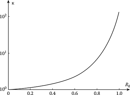
FIGURE 13.1 Variance of the variance estimate versus the true value of the correlation coefficient.

$κ = \frac{1 + 2 ρ_{0}^{2}}{1 - ρ_{0}^{2}} (13.36)$

as a function of the true value ρ₀ of the correlation coefficient is shown in Figure 13.1. The value κ shows how much the variance of variance estimate increases with the increase in the error under definition of the correlation coefficient ρ. As we can see from (13.35) and Figure 13.1, with increase in the absolute value of the correlation coefficient, the errors in variance estimate also rise rapidly. In doing so, if the module of the correlation coefficient between samples tends to approach unit, then independent of the small variance Var_ε of the definition of the correlation coefficient the variance of the variance estimate of stochastic process increases infinitely. Compared to ρ₀ = 0, at |ρ₀| = 0.95, the value κ increases 30 times and at |ρ₀| = 0.99 and |ρ₀| = 0.999, 150 and 1500 times, respectively. For this reason, at sufficiently high values of the module of correlation coefficient between samples we need to take into consideration the variance of definition of the correlation coefficient ρ. Qualitatively, this result is correct in the case of the optimal variance estimate of the Gaussian stochastic process under multidimensional sampling.

Although in applications we define the correlation function with errors, in particular cases, when we carry out a simulation, we are able to satisfy the simulation conditions, in which the normalized correlation function is known with high accuracy. This circumstance allows us to verify experimentally the correctness of the definition of optimal variance estimate of Gaussian stochastic process by sampling with high values given by the module of correlation coefficient between samples.

Experimental investigations of the optimal (13.5) and nonoptimal (13.24) variance estimations by two samples with various values of the correlation coefficient between them were carried out. To simulate various values of the correlation coefficient between samples, the following pair of values was formed:

$x_{i} = \frac{1}{L} {\sum^{}}_{p = 1}^{L} y_{i - p}, (13.37)$

$\begin{matrix} x_{i - k} = \frac{1}{L} {\sum^{}}_{p = 1}^{L} y_{i - k - p}, & k = 0, 1, \dots, L . \end{matrix} (13.38)$

As we can see from (13.37) and (13.38), the samples x_i and x_i-k are the sums of independent samples y_p obtained from the stationary Gaussian stochastic process with zero mathematical expectation.

Images

FIGURE 13.2 Normalized correlation function of stationary Gaussian stochastic process.

The samples x_i and x_i-k are distributed according to the Gaussian pdf and possess zero mathematical expectations. The correlation function between the newly formed samples can be presented in the following form:

$R_{k} = 〈 x_{i} x_{i - k} 〉 = \frac{1}{L^{2}} {\sum^{}}_{p = 1}^{L - | k |} 〈 y_{p}^{2} 〉 = \frac{σ^{2}}{L} (1 - \frac{| k |}{L}) . (13.39)$

To obtain the samples x_i and x_i-k subjected to the Gaussian pdf we use the stationary Gaussian stochastic process with the normalized correlation function presented in Figure 13.2. As we can see from Figure 13.2, the samples of stochastic process y_p with the sampling period exceeding 0.2 ms are uncorrelated practically. In the course of test, to ensure a statistical independence of the samples y_p we use the sampling rate equal to 512 Hz, which is equivalent to 2 ms between samples. Experimental test with the sample size equal to 10⁶ shows that the correlation coefficient between neighboring readings of the sample y_p is not higher than 2.5 × 10⁻³.

Statistical characteristics of estimations given by (13.5) and (13.24) at N = 2 are computed by the microprocessor system. The samples x_i and x_i-k are obtained as a result of summing 100 independent readings of y_i-p and y_i-k-p, respectively, which guarantees a variation of the correlation coefficient from 0 to 1 at the step 0.01 when the value k changes from 100 to 0. The statistical characteristics of estimates of the mathematical expectation 〈Var_j〉 and the variance Var{Var_j} at j = 1 corresponding to the optimal estimate given by (13.5) and at j = 2 corresponding to the estimate given by (13.24) are determined by 3 × 10⁵ pair samples x_i and x_i-k. In the course of this test, the mathematical expectation and variance have been determined based on 10⁶ samples of x_i. In doing so, the mathematical expectation has been considered as zero, not high 1.5 × 10⁻³, and the variance has been determined as σ² = 2.785.

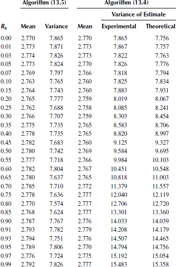
Experimental statistical characteristics of variance estimate obtained with sufficiently high accuracy are matched with theoretical values. The maximal relative errors of definition of the math-ematical expectation estimate and the variance estimate do not exceed 1% and 2.5%, correspondingly Table 13.1 presents the experimental data of the mathematical expectations and variations in the variance estimate at various values of the correlation coefficient ρ₀ between samples. Also, the theoretical data of the variance of the variance estimate based on the algorithm given by (13.24) and determined in accordance with the formula

$Var {{Var}^{*}} = σ^{2} (1 + ρ_{0}^{2}) (13.40)$

are presented for comparison in Table 13.1. Theoretical value of the variance of the optimal variance estimate is equal to Var{Var_E} = 7.756 according to (13.5). Thus, the experimental data prove the previously mentioned theoretical definition of estimates and their characteristics, at least at N = 2.

TABLE 13.1
Experimental Data of Definition of the Mathematical Expectation and Variance of the Variance Estimate

Images

13.2 Stochastic Process Variance Estimate Under Averaging in Time

In practice, under investigation of stationary stochastic processes, the value

${Var}^{*} = {\int^{}}_{0}^{T} h (t) {[x (t) - E]}^{2} d t (13.41)$

is considered as the variance estimate, where x(t) is the realization of observed stochastic process; E is the mathematical expectation; h(t) is the weight function with the optimal form defined based on the condition of unbiasedness of the variance estimate

${\int^{}}_{0}^{T} h (t) d t = 1 (13.42)$

and minimum of the variance of the variance estimate. As applied to the stationary Gaussian stochastic process, the variance of the variance estimate can be presented in the following form:

$Var {{Var}^{*}} = 4 σ^{2} {\int^{}}_{0}^{T} ℛ^{2} (τ) r_{h} (τ) d τ, (13.43)$

when the mathematical expectation is known by analogy with (12.130), where σ² is the true value of variance, ℛ(τ) is the normalized correlation function of the observed stochastic process, and the function r_h(τ) is given by (12.131).

The optimal weight function applied to stochastic process with the exponential normalized correlation function given by (12.13) is discussed in Ref. [3]. The optimal variance estimate in the sense of the rule given by (13.41) and the minimal value of the variance of the variance estimate take the following form:

${Var}_{opt}^{*} = \frac{x_{0}^{2} (0) + x_{0}^{2} (T) + 2 α {\int^{}}_{0}^{T} x^{2} (t) d t}{2 (1 + α T)}; (13.44)$

$Var {{Var}_{opt}^{*}} = \frac{2 σ^{4}}{1 + α T} . (13.45)$

To obtain the considered optimal estimate we need to know the correlation function with high accuracy that is not possible forever. For this reason, as a rule, the weight function is selected based on the simplicity of realization, but the estimate would be unbiased and with increasing observation time interval, the variance of the variance estimate would tend to approach zero monotonically decreased. The function given by (12.112) is widely used as the weight function.

We assume that the investigated stochastic process is a stationary one and the current estimate of the stochastic process variance within the limits of the observation time interval [0, T] has the following value:

${Var}^{*} (t) = \frac{1}{T} {\int^{}}_{0}^{T} {x (τ) - \frac{1}{T} {\int^{}}_{0}^{T} x (z) d z}^{2} = \frac{1}{T} {\int^{}}_{0}^{T} {[x (τ) - E^{*} (t)]}^{2} d τ, (13.46)$

where E*(t) is the mathematical expectation estimate at the instant t. The flowchart of measurer operating in accordance with (13.46) is shown in Figure 13.3.

Images

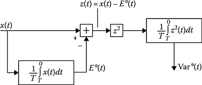
FIGURE 13.3 Flowchart of measurer operating in accordance with (13.46).

Determine the mathematical expectation and the variance of the variance estimate assuming that the investigated stochastic process is a stationary Gaussian process with unknown mathematical expectation. The mathematical expectation of variance estimate is given by

$〈 {Var}^{*} 〉 = \frac{1}{T} {\int^{}}_{0}^{T} 〈 x^{2} (τ) 〉 d τ - \frac{1}{T^{2}} {\int^{}}_{0}^{T} {\int^{}}_{0}^{T} 〈 x (τ_{1}) x (τ_{2}) 〉 d τ_{1} d τ_{2} . (13.47)$

Taking into consideration that

$x_{0} (t) = x (t) - E_{0} (13.48)$

and transforming the double integral into a single one introducing new variables, we obtain

$〈 {Var}^{*} 〉 = σ^{2} {1 - \frac{2}{T} {\int^{}}_{0}^{T} (1 - \frac{τ}{T}) ℛ (τ) d τ} . (13.49)$

As we can see from (13.49), while estimating the variance of stochastic process with the unknown mathematical expectation, there is a bias of estimate defined as

$b {{Var}^{*}} = \frac{2 σ^{2}}{T} {\int^{}}_{0}^{T} (1 - \frac{τ}{T}) ℛ (τ) d τ . (13.50)$

In other words, the bias of variance estimate coincides with the variance of mathematical expectation estimate of stochastic process (12.116). The bias of variance estimate depends on the observation time interval and the correlation function of investigated stochastic process. If the observation time interval is much more than the correlation interval of the investigated stochastic process and the normalized correlation function is not an alternative function, the bias of variance estimate is defined by (12.118).

Analogous effect is observed in the case of sampling the stochastic process. We consider the following value as the estimate of stochastic process variance:

${Var}^{*} = \frac{1}{N - 1} {\sum^{}}_{i = 1}^{N} {x_{i} - \frac{1}{N} {\sum^{}}_{j = 1}^{N} x_{j}}^{2}, (13.51)$

where N is the total number of samples of stochastic process at the instants t = iΔ, i = 1, 2, …, N. The mathematical expectation of variance estimate is determined in the following form:

$〈 {Var}^{*} 〉 = \frac{σ^{2}}{N - 1} {N - \frac{1}{N} {\sum^{}}_{i = 1, k = 1}^{N} ℛ [(i - k) Δ]} . (13.52)$

Carrying out the transformation as it was done in Section 12.5, we obtain

$〈 {Var}^{*} 〉 = σ^{2} {1 - \frac{2}{N - 1} {\sum^{}}_{i = 1}^{N} (1 - \frac{i}{N}) ℛ (i Δ)} . (13.53)$

If the samples are uncorrelated, we have

$〈 {Var}^{*} 〉 = σ^{2} . (13.54)$

In other words, we see from (13.54) that under the uncorrelated samples the variance estimate (13.51) is unbiased.

In a general case of the correlated samples, the bias of estimate of stochastic process variance is given by

$b {{Var}^{*}} = \frac{2 σ^{2}}{N - 1} {\sum^{}}_{i = 1}^{N} (1 - \frac{i}{N}) ℛ (i Δ) . (13.55)$

In doing so, if the number of investigated samples is much more than, the ratio of the correlation interval of stochastic process to the sampling period, (13.55) is simplified and takes the following form:

$b {{Var}^{*}} = \frac{2 σ^{2}}{N - 1} {\sum^{}}_{i = 1}^{N} ℛ (i Δ) . (13.56)$

For measuring the variance of stochastic processes, we can often assume that the mathematical expectation of stochastic process is zero and the variance estimate is carried out based on smoothing the squared stochastic process by the linear filter with the impulse response h(t), namely,

$Var * (t) = \frac{{\int^{}}_{0}^{T} h (τ) x^{2} (t - τ) d τ}{{\int^{}}_{0}^{T} h (τ) d τ} . (13.57)$

If the observation time interval is large, that is, a difference between the instants of estimation and beginning to excite the filter input by stochastic process much more than the correlation interval of the investigated stochastic process and filter time constant, then

${Var}^{*} (t) = \frac{{\int^{}}_{0}^{\infty} h (τ) x^{2} (t - τ) d τ}{{\int^{}}_{0}^{\infty} h (τ) d τ} . (13.58)$

Under sampling the stochastic process with known mathematical expectation, the value

${Var}^{*} = \frac{1}{N} {\sum^{}}_{i = 0}^{N} {(x_{j} - E_{0})}^{2} (13.59)$

is taken as the variance estimate that ensures the estimate unbiasedness.

Let us define the variance of the variance estimate caused by the finite observation time interval of stochastic process. Let the investigated stochastic process be the stationary one and we use the ideal integrator as the smoothing filter. In this case, the variance estimate is carried out in accordance with (13.46) and the variance of the variance estimate takes the following form:

$\begin{array}{l} Var {{Var}^{*}} = & \frac{1}{T^{2}} {\int^{}}^{}_{0}^{T} {\int^{}}^{}_{0}^{T} 〈 x^{2} (t_{1}) x^{2} (t_{2}) 〉 d t_{1} d t_{2} - \frac{2}{T^{3}} {\int^{}}^{}_{0}^{T} {\int^{}}^{}_{0}^{T} {\int^{}}^{}_{0}^{T} 〈 x^{2} (t_{1}) x (t_{2}) x (t_{3}) 〉 d t_{1} d t_{2} d t_{3} \\ + \frac{1}{T^{4}} {\int^{}}^{}_{0}^{T} {\int^{}}^{}_{0}^{T} {\int^{}}^{}_{0}^{T} {\int^{}}^{}_{0}^{T} 〈 x (t_{1}) x (t_{2}) x (t_{3}) x (t_{4}) 〉 d t_{1} d t_{2} d t_{3} d t_{4} - σ^{4} {1 - \frac{2}{T} {\int^{}}^{}_{0}^{T} (1 - \frac{τ}{T}) ℛ (τ) d τ}^{2} . \end{array} (13.60)$

Determination of moments in the integrands (13.60) is impossible for the arbitrary pdf of the investigated stochastic process. For this reason, to define the main regularities we assume that the investigated stochastic process is Gaussian with the unknown mathematical expectation, the true value of which is E₀. Then, after the corresponding transformations, we have

$\begin{array}{l} Var {{Var}^{*}} = & \frac{4 σ^{4}}{T} {{\int^{}}^{}_{0}^{T} (1 - \frac{τ}{T}) ℛ^{2} (τ) d τ + \frac{2}{T} {{\int^{}}^{}_{0}^{T} (1 - \frac{τ}{T}) ℛ (τ) d τ}^{2} \\ - \frac{1}{T^{2}} {\int^{}}^{}_{0}^{T} {\int^{}}^{}_{0}^{T} {\int^{}}^{}_{0}^{T} ℛ (t_{1} - t_{2}) ℛ (t_{1} - t_{3}) d t_{1} d t_{2} d t_{3}} . \end{array} (13.61)$

If the mathematical expectation of the investigated stochastic process is known accurately, then according to (13.46) the variance estimate is unbiased and the variance of the variance estimate takes the following form:

$Var {{Var}^{*}} = \frac{4 σ^{4}}{T} {\int^{}}_{0}^{T} (1 - \frac{τ}{T}) ℛ^{2} (τ) d τ . (13.62)$

When the observation time interval is sufficiently large, that is, the condition T ≫ τ_cor is satisfied, (13.62) is simplified and takes the following form:

$Var {{Var}^{*}} \approx \frac{4 σ^{4}}{T} {\int^{}}_{0}^{\infty} ℛ^{2} (τ) d τ \leq \frac{4 σ^{4} τ_{cor}}{T} . (13.63)$

Using (12.27) and (12.122), at the condition T ≫ τ_cor, variance of the variance estimate can be presented in the following form:

$Var {{Var}^{*}} \approx \frac{2}{T} \int_{- \infty}^{\infty} R^{2} (τ) d τ = \frac{2}{π T} {\int^{}}_{0}^{\infty} S^{2} (ω) d ω . (13.64)$

As applied to the exponential correlation function given by (12.13), the normalized variance of the variance estimate can be presented in the following form:

$\frac{Var {{Var}^{*}}}{σ^{4}} = \frac{2 p - 1 + \exp {- 2 p}}{p^{2}}, (13.65)$

where p is given by (12.48). Analogous formulae for the variance of the variance estimate can be obtained when the stochastic process is sampling. Naturally, at that time, the simplest expressions are obtained in the case of independent readings of the investigated stochastic process.

Determine the variance of the variance estimate of stochastic process according to (13.51) for the case of independent samples. For this case, we transform (13.51) in the following form:

${Var}^{*} = \frac{1}{N - 1} {{\sum^{}}^{}_{i = 1}^{N} y_{i}^{2} - \frac{1}{N} {{\sum^{}}^{}_{p = 1}^{N} y_{p}}^{2}}, (13.66)$

where y_i = x_i − E. As we can see, the variance estimate is unbiased. The variance of the variance estimate of stochastic process can be determined in the following form:

$Var {{Var}^{*}} = \frac{1}{{(N - 1)}^{2}} {{\sum^{}}^{}_{i = 1, j = 1}^{N} 〈 y_{i}^{2} y_{j}^{2} 〉 - \frac{2}{N} {\sum^{}}^{}_{i = 1, p = 1, q = 1}^{N} 〈 y_{i}^{2} y_{p} y_{q} 〉 + \frac{1}{N^{2}} {\sum^{}}^{}_{i = 1, j = 1, p = 1, q = 1}^{N} 〈 y_{i} y_{j} y_{p} y_{q} 〉} - σ^{4} . (13.67)$

To compute the sums in the brackets we select the terms with the same indices. Taking into consideration the independence of the samples, we have

${\sum^{}}_{i = 1, j = 1}^{N} 〈 y_{i}^{2} y_{j}^{2} 〉 = {\sum^{}}_{i = 1}^{N} 〈 y_{i}^{4} 〉 + {\sum^{}}_{i = 1, j = 1, i \neq j}^{N} 〈 y_{i}^{2} 〉 〈 y_{j}^{2} 〉 = N μ_{4} + N (N - 1) μ_{2}^{2}, (13.68)$

where

$μ_{v_{i}} = 〈 y_{i}^{v} 〉 = 〈 {(x_{j} - E)}^{v} 〉 (13.69)$

is the central moment of the vth order and, naturally, μ₂ = σ². Analogously, we obtain

${\sum^{}}_{i = 1, p = 1, q = 1}^{N} 〈 y_{i}^{2} y_{p} y_{q} 〉 = N μ_{4} + N (N - 1) μ_{2}^{2}; (13.70)$

${\sum^{}}_{i = 1, j = 1, p = 1, q = 1}^{v} 〈 y_{i} y_{j} y_{p} y_{q} 〉 = N μ_{4} + 3 N (N - 1) μ_{2}^{2} . (13.71)$

Substituting (13.70) and (13.71) into (13.67), we obtain

$Var {{Var}^{*}} = \frac{μ_{4} - {1 - (2 / (N - 1))} σ^{2}}{N} . (13.72)$

In the case of Gaussian stochastic process we have μ₄ = 3σ⁴. As a result we obtain

$Var {{Var}^{*}} = \frac{2 σ^{4}}{N - 1} . (13.73)$

If the mathematical expectation is known, then the unbiased variance estimate is defined as

${Var}^{*} = \frac{1}{N} {\sum^{}}_{i = 1}^{N} {(x_{i} - E_{0})}^{2}, (13.74)$

and the variance of the variance estimate takes the following form:

$Var {{Var}^{*}} = \frac{μ_{4} - 0^{4}}{N} . (13.75)$

In the case of Gaussian stochastic process, variation in the variance estimate has the following form:

$Var {{Var}^{*}} = \frac{2 σ^{4}}{N} . (13.76)$

Comparing (13.76) with (13.73), we can see that at N ≫ 1 these formulas are coincided.

As applied to the iterative variance estimate of stochastic process with zero mathematical expectation, based on (12.342) and (12.345) we obtain

In the case of discrete stochastic process

${Var}^{*} {N} = {Var}^{*} [N - 1] + γ [N] {x^{2} [N] - {Var}^{*} [N - 1]}; (13.77)$
In the case of continuous stochastic process

$\frac{d {Var}^{*} (t)}{d t} = γ (t) {x^{2} (t) - {Var}^{*} (t)} . (13.78)$

As shown in Section 12.9, we can show that the optimal value of the factor γ[N] is equal to N⁻¹.

13.3 Errors Under Stochastic Process Variance Estimate

As we can see from formulas for the variance estimate of stochastic process, a squaring of the stochastic process realization (or its samples) is a very essential operation. The device carrying out this operation is called the quadratic transformer or quadrator. The difference in quadrator performance from square-law function leads to additional errors arising under measurement of the stochastic process variance. To define a character of these errors we assume that the stochastic process possesses zero mathematical expectations and the variance estimate is carried out based on investigation of independent samples. The characteristic of transformation y = g(x) can be presented by the polynomial function of the μth order

$y = g (x) = {\sum^{}}_{k = 0}^{μ} a_{k} x^{k} . (13.79)$

Substituting (13.79) into (13.59) instead of x_i and carrying out averaging, we obtain the mathematical expectation of variance estimate:

$〈 {Var}^{*} 〉 = {\sum^{}}_{k = 0}^{μ} a_{k} 〈 x^{k} 〉 = a_{0} + a_{2} σ^{2} + {\sum^{}}_{k = 3}^{μ} a_{k} 〈 x^{k} 〉 . (13.80)$

The estimate bias caused by the difference between the transformation characteristic and the square-law function can be presented in the following form:

$b {{Var}^{*}} = σ^{4} (a_{2} - 1) + a_{0} + {\sum^{}}_{k = 3}^{μ} a_{k} 〈 x^{k} 〉 . (13.81)$

For the given transformation characteristic the coefficients a_k can be defined before. For this reason, the bias of variance estimate caused by the coefficients a₀ and a₂ can be taken into consideration. The problem is to take into consideration the sum in (13.81) because this sum depends on the shape of pdf of the investigated stochastic process:

$〈 x^{k} 〉 = \int_{- \infty}^{\infty} x^{k} f (x) d x . (13.82)$

In the case of Gaussian stochastic process, the moment of the kth order can be presented in the following form:

$〈 x^{k} 〉 = {\begin{array}{l} 1 \cdot 3 \cdot 5... (k - 1) σ^{0.5 k}, & if k is even; \\ 0, & if k is odd; \end{array} (13.83)$

Difference between the transformation characteristic and the square-law function can lead to high errors under definition of the stochastic process variance. Because of this, while defining the stochastic process variance we need to pay serious attention to transformation performance. Verification of the transformation performance is carried out, as a rule, by sending the harmonic signal of known amplitude at the measurer input.

While measuring the stochastic process variance, we can avoid the squaring operation. For this purpose, we need to consider two sign functions (12.208)

${\begin{matrix} η_{1} (t) = s g n [ξ (t) - μ_{1} (t)] \\ η_{2} (t) = s g n [ξ (t) - μ_{2} (t)] \end{matrix}, (13.84)$

instead of the initial stochastic process ξ(t) with zero mathematical expectation, where μ(t) and μ₂(t) are additional independent stationary stochastic processes with zero mathematical expectations and the same pdf given by (12.205). At the same time, the condition given by (12.206) is satisfied.

The functions η₁(t) and η₂(t) are the stationary stochastic processes with zero mathematical expectations. In doing so, if the fixed value ξ(t) = x the conditional stochastic processes η₁(t|x) and η₂(t|x) are statistically independent, that is,

$〈 η_{1} (t | x) η_{2} (t | x) 〉 = 〈 η_{1} (t | x) 〉 〈 η_{2} (t | x) 〉 . (13.85)$

Taking into consideration (12.209), we obtain

$〈 η_{1} (t | x) η_{2} (t | x) 〉 = \frac{x^{2}}{A^{2}} . (13.86)$

The unconditional mathematical expectation of product can be presented in the following form:

$〈 η_{1} (t | x) η_{2} (t | x) 〉 = \frac{1}{A^{2}} \int_{- \infty}^{\infty} x^{2} p (x) d x = \frac{σ^{2}}{A^{2}} . (13.87)$

Denote the realizations of stochastic processes η₁(t) and η₂(t) by the functions y₁(t) and y₂(t), respectively. Consequently, if we consider the following value as the variance estimate,

$\tilde{Var} = \frac{A^{2}}{T} {\int^{}}_{0}^{T} y_{1} (t) y_{2} (t) d t, (13.88)$

then the variance estimate is unbiased.

The realizations y₁(t) and y₂(t) take the values equal to ±1. For this reason, the multiplication and integration in (13.88) can be replaced by individual integration of new unit functions obtained as a result of coincidence and noncoincidence of polarities of the realizations y₁(t) and y₂(t):

${\int^{}}_{0}^{T} y_{1} (t) y_{2} (t) d t = {\int^{}}_{0}^{T} z_{1} (t) d t - {\int^{}}_{0}^{T} z_{2} (t) d t, (13.89)$

where

$z_{1} (t) = {\begin{array}{l} 1 & if {\begin{matrix} y_{1} (t) > 0, y_{2} (t) > 0; \\ y_{1} (t) < 0, y_{2} (t) < 0; \end{matrix} \\ 0 & otherwise; \end{array} (13.90)$

$z_{2} (t) = {\begin{array}{l} 1 & if {\begin{matrix} y_{1} (t) > 0, y_{2} (t) < 0; \\ y_{1} (t) < 0, y_{2} (t) > 0; \end{matrix} \\ 0 & otherwise . \end{array} (13.91)$

Images

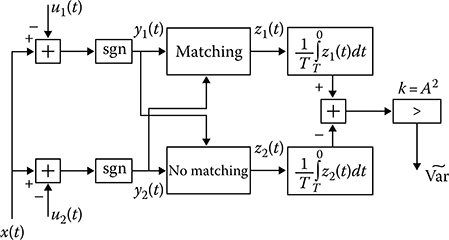
FIGURE 13.4 Measurer based on additional signals.

The flowchart of measuring device based on the implementation of additional signals is shown in Figure 13.4.

In the case of discrete process, the variance estimate can be presented in the following form:

$\tilde{Var} = \frac{A^{2}}{N} {\sum^{}}_{i = 1}^{N} y_{1_{i}} y_{2_{i}}, (13.92)$

where y_{1_i} = y₁(t_i) and y₂ = y₂(t_i). In this case, the integrator can be replaced by the summator in Figure 13.4.

Determine the variance of the variance estimate $\tilde{Var}$ applied to investigation of stochastic process at discrete instants for the purpose of simplifying further analysis that the samples y_1i and y_2i are independent. Otherwise, we should know the two-dimensional pdfs of additional uniformly distributed stochastic processes μ₁(t) and μ₂(t). The variance of the variance estimate can be presented in the following form:

$Var {\tilde{Var}} = \frac{A^{4}}{N^{2}} \sum_{i = 1, j = 1}^{N} 〈 y_{1_{i}} y_{1_{j}} y_{2_{i}} y_{2_{j}} 〉 - {〈 \tilde{Var} 〉}^{2} . (13.93)$

In double sum, we can select the terms with i = j. Then

${\sum^{}}_{i = 1, j = 1}^{N} 〈 y_{1_{i}} y_{1_{j}} y_{2_{i}} y_{2_{j}} 〉 = {\sum^{}}_{i = 1}^{N} 〈 {(y_{1_{i}} y_{2_{i}})}^{2} 〉 + {\sum^{}}_{i = 1, j = 1, i \neq j}^{N} 〈 y_{1_{i}} y_{1_{j}} y_{2_{i}} y_{2_{j}} 〉, (13.94)$

where

$〈 y_{1_{i}} y_{1_{j}} y_{2_{i}} y_{2_{j}} 〉 = 〈 η_{1_{i}} η_{1_{j}} η_{2_{i}} η_{2_{j}} 〉 . (13.95)$

Based on a definition of sign functions, we can obtain from (13.84) the following condition:

${[y_{1} (t) y_{2} (t)]}^{2} = 1. (13.96)$

Define the cumulative moment 〈η_{1_i}η_{1_j}η_{2_i}η_{2_j}|x_ix_j〉 at the condition that ξ(t_i) = x_i and ξ(t_j) = x_j. Taking into consideration the statistical independence of the samples η₁ and η₂, the statistical mutual independence of the stochastic values η₁(t|x) and η₂(t|x), and (12.209), the conditional cumulative moment can be presented in the following form:

$〈 η_{1_{i}} η_{1_{j}} η_{2_{i}} η_{2_{j}} | x_{j} x_{j} 〉 = \frac{x_{i}^{2} x_{j}^{2}}{A^{4}} . (13.97)$

Averaging (13.97) by possible values of independent random variables x_i and x_j, we obtain

$〈 η_{1_{i}} η_{1_{j}} η_{2_{i}} η_{2_{j}} 〉 = \frac{〈 x_{i}^{2} x_{j}^{2} 〉}{A^{4}} = \frac{〈 x_{i}^{2} 〉 〈 x_{j}^{2} 〉}{A^{4}} = \frac{σ^{4}}{A^{4}} . (13.98)$

Substituting (13.96) and (13.98) into (13.93), we obtain the variance of the variance estimate (13.92)

$Var {{Var}^{•}} = \frac{A^{4}}{N} (1 - \frac{σ^{4}}{A^{4}}) . (13.99)$

The variance estimate according to (13.92) envisages that the condition (12.206) is satisfied. Consequently, the inequality σ² ≪ A² must be satisfied. Because of this, as in the case of estimation of the mathematical expectation with employment of additional signals, the variance of the variance estimate $\tilde{Var}$ is completely defined by the half intervals of possible values of additional random sequences. Comparing the obtained variance (13.99) with the variance of the variance estimate in (13.76) by N independent samples, we can find that

$\frac{Var {\tilde{Var}}}{Var {{Var}^{*}}} = \frac{A^{4}}{2 σ^{4}} (1 - \frac{σ^{4}}{A^{4}}) . (13.100)$

Thus, we can conclude that the method of measurement of the stochastic process variance using the additional signals is characterized by the higher variance compared to the algorithm (13.74). This is based on the example of definition of the variance estimate of stochastic sample with the uniform pdf coinciding with (12.205), σ² = A²/3. As a result, we have

$\frac{Var {\tilde{Var}}}{Var {{Var}^{*}}} = 4. (13.101)$

The methods that are used to measure the variance assume the absence of limitations of instantaneous values of the investigated stochastic process. The presence of these limitations leads to additional errors while measuring the variance. Determine the bias of variance estimate of the Gaussian stochastic process when there is a limiter of the type (12.151) presented in Figure 12.6 applied to zero mathematical expectation and the true value of the variance σ². The variance estimate is defined by (13.41). The ideal integrator h(t) = T⁻¹ plays a role in averaging or smoothing filter. Substituting the realization y(t) = g[x(t)] into (13.41) instead of x(t) and carrying out averaging of the obtained formula with respect to x(t), the bias of variance estimate of Gaussian stochastic process can be written in the following form:

$b {Var} * = \int_{- \infty}^{\infty} g^{2} (x) p (x) d x - σ^{2} = - 2 σ^{2} {(1 - γ^{2}) Q (γ) - \frac{γ}{\sqrt{2 π}} \exp {- 0.5 γ^{2}}}, (13.102)$

Images

FIGURE 13.5 Bias of variance estimate of Gaussian stochastic process as a function of the normalized limitation level.

where

$γ = \frac{a}{σ} (13.103)$

is the normalized limitation level. At γ ≫ 1, we obtain that the bias of variance estimate tends to approach zero, which is expected. The bias of variance estimate of Gaussian stochastic process as a function of the normalized limitation level is shown in Figure 13.5.

13.4 Estimate of Time-Varying Stochastic Process Variance

To define the current value of nonstationary stochastic process variance there is a need to have a set of realizations x_i(t) of this process. Then the variance estimate of stochastic process at the instant t₀ can be presented in the following form:

${Var}^{*} (t_{0}) = \frac{1}{N} {\sum^{}}_{i = 1}^{N} {[x_{j} (t_{0}) - E (t_{0})]}^{2}, (13.104)$

where

N is the number of realizations x_i(t) of stochastic process
E(t₀) is the mathematical expectation of stochastic process at the instant t₀

As we can see from (13.104), the variance estimate is unbiased and the variance of the variance estimate under observation of N independent realizations can be presented in the following form:

$Var {{Var}^{*} (t_{0})} = \frac{{Var}^{2} (t_{0})}{N}; (13.105)$

that is, the variance estimate according to (13.104) is the consistent estimate.

In most cases, the researcher defines the variance estimate on the basis of investigation of a single realization of stochastic process. While estimating time-varying variance based on a single realization of time-varying stochastic process, there are similar problems as seen with the estimation of the time-varying mathematical expectation. On the one hand, to decrease the variance estimate caused by the finite observation time interval, the last must be as soon as large. On the other hand, we need to choose the integration time as short as possible for the best definition of variations in variance. Evidently, there must be a compromise.

The simplest way to define the time-varying stochastic process variance at the instant t₀ is averaging the transformed input data of stochastic process within the limits of finite time interval. Thus, let x(t) be the realization of stochastic process ξ(t) with zero mathematical expectation. Measurement of variance of this stochastic process at the instant t₀ is carried out by averaging the quadrature ordinates x(t) within the limits of the interval about the given value of argument [t₀ − 0.5T, t₀ + 0.5T]. In this case, the variance estimate takes the following form:

${Var}^{*} (t_{0}, T) = \frac{1}{T} {\int^{}}_{t_{0} - 0.5 T}^{t_{0} + 0.5 T} x^{2} (t) d t = \frac{1}{T} {\int^{}}_{- 0.5 T}^{0.5 T} x^{2} (t + t_{0}) d t . (13.106)$

Averaging the variance estimate by realizations, we obtain

$〈 {Var}^{*} (t_{0}, T) 〉 = \frac{1}{T} {\int^{}}_{- 0.5 T}^{0.5 T} Var (t + t_{0}) d t . (13.107)$

Thus, as in the case of time-varying mathematical expectation, the estimate of the variance of the time-varying mathematical expectation does not coincide with its true value in a general case, but it is obtained by smoothing the variance within the limits of finite time interval [t₀ − 0.5T, t₀ + 0.5T]. As a result of such averaging, the bias of variance of stochastic process can be presented in the following form:

$b {{Var}^{*} (t_{0}, T)} = \frac{1}{T} {\int^{}}_{- 0.5 T}^{0.5 T} [Var (t + t_{0}) - Var (t_{0})] d t . (13.108)$

If we would like to have the unbiased estimate, a variance of the variance Var(t) within the limits of time interval.[t₀ − 0.5T, t₀ + 0.5T] must be the odd function and, in the simplest case, the linear function of time

$\begin{matrix} Var (t_{0} + t) \approx Var (t_{0}) + Var' (t_{0}) t, & - 0.5 T \leq t \leq 0.5 T . \end{matrix} (13.109)$

Evaluate the influence of deviation of the current variance Var(t) from linear function on its estimate. In doing so, we assume that the estimated current variance has the continuous first and second derivatives with respect to time. Then, according to the Taylor expansion we can write

$Var (t) = Var (t_{0}) + (t - t_{0}) + Var' (t) + 0.5 (t - t_{0}) Var ″ [t_{0} + θ (t - t_{0})], (13.110)$

where 0 < θ < 1. Substituting (13.110) into (13.108), we obtain

$b {{Var}^{*} (t_{0}, T)} = \frac{1}{2 T} {\int^{}}_{- 0.5 T}^{0.5 T} t^{2} Var ″ (t_{0} + t θ) d t . (13.111)$

Denoting M_Var the maximal absolute value of the second derivative of the current variance Var(t) with respect to time, we obtain the high bound value of the variance estimate bias by absolute value

$| b {{Var}^{*} (t_{0}, T)} | \leq \frac{T^{2} M_{Var}}{24} . (13.112)$

The maximum value of the second derivative of the time-varying variance Var(t) can be evaluated, as a rule, based on the analysis of specific physical problems.

To estimate the difference in the time-varying variance a square of the investigated realization of the stochastic process can be presented in the following form of two sums:

$ξ^{t} (t) = Var + (t) + ζ (t), (13.113)$

where

Var(t) is the true value of the stochastic process variance at the instant t
ζ(t) are the fluctuations of square of the stochastic process realization with respect to its math-ematical expectation at the same instant t

Then the variation in the variance estimate of the investigated nonstationary stochastic process can be presented in the following form:

$Var {{Var}^{*} (t_{0}, T)} = \frac{1}{T^{2}} {\int^{}}_{- 0.5 T}^{0.5 T} {\int^{}}_{- 0.5 T}^{0.5 T} R_{ζ} (t_{1} + t_{0}, t_{2} + t_{0}) d t_{1} d t_{2}, (13.114)$

where

$R_{ζ} (t_{1}, t_{2}) = 〈 [x^{2} (t_{1}) - Var (t_{1})] [x^{2} (t_{2}) - Var (t_{2})] 〉 (13.115)$

is the correlation function of the random component of the investigated squared stochastic process with respect to its variance at the instant t.

To define the approximate value of the variance of slowly varying in time variance estimate we can assume that the centralized stochastic process ζ(t) within the limits of the finite time interval [t₀ − 0.5T, t₀ + 0.5T] is the stationary stochastic process with the correlation function defined as

$R_{ζ} (t, t + τ) \approx {Var}_{ζ} (t_{0}) ℛ_{ζ} (τ) . (13.116)$

Taking into consideration the approximation given by (13.116), the variance of the variance estimate presented in (13.114) can be presented in the following form:

$Var {{Var}^{*} (t_{0}, T)} = {Var}_{ζ} (t_{0}) \frac{2}{T} {\int^{}}_{0}^{T} (1 - \frac{τ}{T}) ℛ_{ζ} (τ) d τ . (13.117)$

As applied to the Gaussian stochastic process at the given assumptions, we can write

$R_{ζ} (t, t + τ) \approx 2 σ^{4} (t_{0}) ℛ^{2} (τ), (13.118)$

and the variance of the variance estimate at the instant t₀ takes the following form:

$Var {{Var}^{*} (t_{0}, T)} = \frac{4 σ^{4} (t_{0})}{T} {\int^{}}_{0}^{T} (1 - \frac{τ}{T}) ℛ^{2} (τ) d τ . (13.119)$

Consider the characteristics of the estimate of the time-varying stochastic process variance for the case, when the investigated stochastic process variance can be presented in the series expansion form

$Var (t) \approx {\sum^{}}_{i = 1}^{N} β_{i} ψ_{j} (t), (13.120)$

where

β_i are some unknown numbers
ψ_i(t) are the given functions of time

With increase in the number of terms in series given by (13.120), the approximation errors can decrease to an infinitesimal value. Similar to (12.258), we can conclude that the coefficients β_i are defined by the system of linear equations

$\begin{matrix} {\sum^{}}_{i = 1}^{N} β_{j} {\int^{}}_{0}^{T} ψ_{i} (t) ψ_{j} (t) d r = {\int^{}}_{0}^{T} Var (t) ψ_{j} (t) d t, & j = 1, 2, ..., N \end{matrix} (13.121)$

based on the condition of minimum of quadratic error of approximation (13.120). Thus, the problem with definition of the stochastic process variance estimate by a single realization observed within the limits of the interval [0, T] can be reduced to estimation of the coefficients β_i in the series given by (13.120). In doing so, the bias and the variance of the variance estimate of the investigated stochastic process caused by errors occurring while measuring the coefficients β_i take the following form:

$b {{Var}^{*} (t)} = Var (t) - {Var}^{*} (t) = {\sum^{}}_{i = 1}^{N} ψ_{j} (t) [β_{j} - 〈 β_{j}^{*} 〉], (13.122)$

$Var {V a r^{*} (t)} = {\sum^{}}_{i = 1, j = 1}^{v} ψ_{i} (t) ψ_{j} (t) 〈 (β_{i} - β_{j}^{*}) (β_{j} - β_{j}^{*}) 〉 . (13.123)$

The bias and the variance of the variance estimate averaged within the limits of the time interval of observation of stochastic process can be presented in the following form, respectively:

$b {{Var}^{*} (t)} = \frac{1}{T} {\sum^{}}_{i = 1}^{N} [β_{j} - 〈 β_{j}^{*} 〉] {\int^{}}_{0}^{T} ψ_{i} (t) d t, (13.124)$

$Var {{Var}^{*} (t)} = \frac{1}{T} {\sum^{}}_{i = 1, j = 1}^{N} 〈 (β_{j} - β_{j}^{*}) (β_{j} - β_{j}^{*}) 〉 {\int^{}}_{0}^{T} ψ_{i} (t) ψ_{j} (t) d t . (13.125)$

The values minimizing the function

$ε^{2} (β_{1}, β_{2}, ..., β_{N}) = \frac{1}{T} {\int^{}}_{0}^{T} {x^{2} (t) - {\sum^{}}_{i = 1}^{N} β_{i} ψ_{j} (t)}^{2} d t (13.126)$

can be considered as estimations of the coefficients β_i. As we can see from (13.126), the estimation of the coefficients β_i is possible if we have a priori information that Var(t) and ψ_i(t) are slowly varying in time functions compared to the averaged velocity of component

$z (t) = x^{2} (t) - Var (t) . (13.127)$

The function z(t) is the realization of stochastic process ζ(t) and possesses zero mathematical expectation. In other words, (13.126) is true for the definition of coefficients β_i if the frequency band Δf_Var of the time-varying variance is lower than the effective spectrum bandwidth of the investigated stochastic process ζ(t). This fact corresponds to the case when the correlation function of the investigated stochastic process can be written in the following form:

$R (t, t + τ) \approx Var (t) ℛ (t) . (13.128)$

The following stochastic process corresponds to this correlation function:

$ξ (r) = a (t) η (t), (13.129)$

where

η(t) is the stationary stochastic process
a(t) is the slow time-varying deterministic function time in comparison with the function η(t)

Based on the condition of minimum of the function ε², that is,

$\frac{\partial ε^{2}}{\partial β_{m}} = 0, (13.130)$

we obtain the system of equations to estimate the coefficients β_m

$\begin{matrix} {\sum^{}}_{i = 1}^{N} β_{i}^{*} {\int^{}}_{0}^{T} ψ_{i} (t) ψ_{m} (t) d t = {\int^{}}_{0}^{T} x^{2} (t) ψ_{m} (t) d t, & m = 1, 2, ..., N . \end{matrix} (13.131)$

Denote

${\int^{}}_{0}^{T} ψ_{i} (t) ψ_{m} (t) d t = c_{i m}; (13.132)$

${\int^{}}_{0}^{T} x^{2} (t) ψ_{m} (t) d t = y_{m} . (13.133)$

Then

$\begin{matrix} β_{m}^{*} = \frac{1}{A} {\sum^{}}_{i = 1}^{N} A_{i m} y_{i} = \frac{A_{m}}{A}, & m = 1, 2, ..., N, \end{matrix} (13.134)$

where the determinant A of linear equation system (13.131) and the determinant A_p are defined in accordance with (12.270) and (12.271).

Flowchart of measurer of the time-varying variance Var(t) of the investigated stochastic process is shown in Figure 13.6. The measurer operates in the following way. The coefficients c_ij are generated by the generator “Gen_c” in accordance with (13.132) based on the functions ψ_i(t) that are issued by the generator “Gen_ψ.”. Microprocessor system solves the system of linear equations with respect to the estimations $β_{i}^{*}$ of coefficients β_i based on the coefficients c_ij and values y_i obtained according to (13.133). The estimate of time-varying variance Var*(t) is formed based on previously obtained data. The variance estimate has a delay T + ΔT with respect to the true value, and this delay is used to compute the values y_i and to solve the system of N linear equations, respectively. The delay blocks denoted as T and ΔT are used for this purpose. Definition of coefficient estimations $β_{i}^{*}$ is essentially simplified if the functions ψ_i( t) are orthonormalized:

${\int^{}}_{0}^{T} ψ_{i} (t) ψ_{j} (t) d t = {\begin{array}{l} 1 & if & i = j, \\ 0 & if & i \neq j . \end{array} (13.135)$

Images

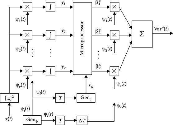
FIGURE 13.6 Measurer of variance in time.

In this case, the series coefficient estimations are defined by a simple integration of the quadratic realization of stochastic process with the corresponding weight function ψ_m(t):

$β_{m}^{*} = {\int^{}}_{0}^{T} x^{2} (t) ψ_{m} (t) d t . (13.136)$

In doing so, the flowchart presented in Figure 13.6 is essentially simplified because there is no need to generate the coefficients c_ij and to solve the system of linear equations. The number of delay block is decreased too.

Determine the bias and mutual correlation functions between the estimates $β_{m}^{*}$ and $β_{q}^{*}$ . Taking into consideration (13.127) we can rewrite (13.133) in the following form:

$y_{i} = {\int^{}}_{0}^{T} z (t) ψ_{i} (t) d t + {\int^{}}_{0}^{T} Var (t) ψ_{i} (t) d t = g_{i} + β_{m} c_{i m} + \underset{q = 1, q \neq m}{\sum^{}} β_{q} c_{i q}, (13.137)$

where

$g_{i} = {\int^{}}_{0}^{T} z (t) ψ_{j} (t) d t . (13.138)$

As in Section 12.7, we can write the estimate $β_{m}^{*}$ of the coefficients in the following form:

$\begin{matrix} β_{m}^{*} = \frac{1}{A} {\sum^{}}_{i = 1}^{N} g_{i} A_{i m} + β_{m}, & m = 1, 2, ..., N, \end{matrix} (13.139)$

where A_im are the algebraic complement of the determinant A_m ≡ B_m (12.276) in which c_ip and g_i are given by (13.132) and (13.138).

Since 〈ζ(t)〉 = 0, then 〈g_i〉 = 0 and, consequently, the estimations $β_{m}^{*}$ of the coefficients in series given by (13.120) are unbiased. The correlation functions $R (β_{m}^{*}, β_{q}^{*})$ and the variance Var( $β_{m}^{*}$ ) are defied by formulas that are analogous to (12.333) and (12.334). For these formulas, we have

$B_{i j} = {\int^{}}_{0}^{T} {\int^{}}_{0}^{T} 〈 z (t_{1}) z (t_{2}) 〉 ψ_{i} (t_{1}) ψ_{j} (t_{2}) d t_{1} d t_{2} = {\int^{}}_{0}^{T} {\int^{}}_{0}^{T} ℛ_{ζ} (t_{1}, t_{2}) ψ_{i} (t_{1}) ψ_{j} (t_{2}) d t_{1} d t_{2} . (13.140)$

We can show that by applying the correlation function R(t₁, t₂) to the Gaussian stochastic process we have

$R_{ζ} (t_{1}, t_{2}) = 2 R^{2} (t_{1}, t_{2}) . (13.141)$

If the functions ψ_i(t) are the orthonormalized functions the correlation function of the estimations $β_{m}^{*}$ and $β_{q}^{*}$ of coefficients is defined by analogy with (12.338):

$R (β_{m}^{*}, β_{q}^{*}) = B_{m q} . (13.142)$

At that time, the formulas for the current and averaged variance of the time-varying variance estimate can be presented as in (12.339) and (12.240)

$Var {{Var}^{*} (t)} = {\sum^{}}_{i = 1, j = 1}^{N} B_{i j} ψ_{i} (t) ψ_{j} (t), (13.143)$

$Var {{Var}^{*}} = \frac{1}{T} {\sum^{}}_{i = 1}^{N} B_{i j} . (13.144)$

If in addition to the condition of orthonormalization of the functions ψ_i(t), we assume that the frequency band of time-varying variance is much lower than the effective spectrum bandwidth of the investigated stochastic process ξ(t), the correlation function of the centralized stochastic process ζ(t) can be presented in the following form:

$R_{ζ} (t_{1}, t_{2}) \approx Var (t_{1}) δ (t_{1} - t_{2}) . (13.145)$

Then, in the case of arbitrary functions ψ_i(t), based on (13.140), we obtain

$B_{i j} = {\int^{}}_{0}^{T} Var (t) ψ_{i} (t) ψ_{j} (t) d t . (13.146)$

If the functions ψ_i( t) are the orthonormalized functions satisfying the Fredholm equation of the second type

$ψ_{i} (t) = λ_{j} {\int^{}}_{0}^{T} R_{ζ} (t_{1}, t_{2}) ψ_{i} (τ) d τ, (13.147)$

we obtain from (13.140) that

$B_{i j} = {\begin{array}{l} \frac{1}{λ_{i}} & if i = j, \\ 0 & if i \neq j . \end{array} (13.148)$

In doing so, the variance of estimations $β_{m}^{*}$ of the coefficients and the current and averaged variations in the variance estimate can be presented in the following form:

$Var {β_{m}^{*}} = \frac{1}{λ_{m}}, (13.149)$

$Var {{Var}^{*} (t)} = {\sum^{}}_{i = 1}^{N} \frac{ψ_{i}^{2} (t)}{λ_{j}}, (13.150)$

$Var {{Var}^{*}} = \frac{1}{T} {\sum^{}}_{i = 1}^{N} \frac{1}{λ_{i}} . (13.151)$

As we can see from (13.151), at the fixed time interval T, with increasing number of terms under approximation of the variance Var(t) by the series given by (13.120) the averaged variance of time-varying variance estimate increases, too.

13.5 Measurement of Stochastic Process Variance in Noise

The specific receivers called the radiometer-type receiver are widely used to measure the variance or power of weak noise signals [4]. Minimal increment in the variance of the stochastic signal is defined by the threshold of sensitivity. In doing so, the threshold of sensitivity of methods that measure the stochastic process variance is called the value of the investigated stochastic process variance equal to the root-mean-square deviation of measurement results. The threshold of sensitivity of radiometer depends on many factors, including the intrinsic noise and random parameters of receiver and the finite time interval of observation of input stochastic process.

Radiometers are classified into four groups by a procedure to measure the stochastic process variance: compensation method, method of comparison with variance of reference source, correlation method, and modulation method. Discuss briefly a procedure to measure the variance of stochastic process by each method.

13.5.1 COMPENSATION METHOD OF VARIANCE MEASUREMENT

Flowchart of compensation method to measure the stochastic process variance is shown in Figure 13.7. While carrying out the compensation method, the additive mixture of the realization s(t) of the investigated stochastic process ζ(t) and the realization n(t) of the noise ς(t) is amplified and squared. The component z(t) that is proportional to the variance of total signal is selected by the smoothing low-pass filter (or integrator). In doing so, the constant component z_const formed by the intrinsic noise of amplifer is essentially compensated by constant bias of voltage or current. There is a need to note that under amplifer we understand the amplifers of radio and intermediate frequencies.

Under practical realization of compensation method to measure the stochastic process variance, the squarer, low-pass filter, and compensating device are often realized as a single device based on the lattice network and the squarer transformer is included in one branch of this lattice network. Branches of lattice network are chosen in such a way that a diagonal indicator could present zero voltage, for example, when the investigated stochastic process is absent. Presence of slow variations in the variance of intrinsic receiver noise and random variations of amplifer coefficient leads to imbalance in the compensation condition that, naturally, decreases the sensitivity of compensation method to measure the stochastic process variance. We consider the low-pass filter as an ideal integrator with the integration time equal to T for obtaining accurate results.

Images

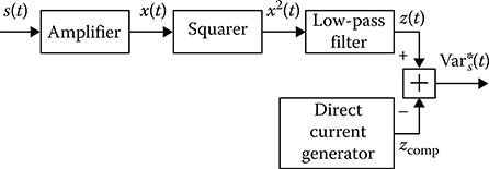
FIGURE 13.7 Compensation method.

Define the dependence of the variation in the stochastic process variance estimate on the main characteristics of investigated stochastic process at the measurer input by the compensation method. We assume that the measurement errors of compensating device are absent with the compensation of the amplifer noise constant component and the spectral densities of the investigated and measured stochastic process ζ(t) and receiver noise c,(t) are distributed uniformly within the limits of amplifer bandwidth.

The realization x(t) of stochastic process ξ(t) at the squarer input can be presented in the following form:

$x (t) = [1 + υ (t)] [s (t) + n (t)] (13.152)$

accurate within the constant coefficient characterizing the average value of amplifer coefficient, where υ(t) is the realization of random variations of the receiver amplifer coefficient β(t). Since the amplifer coefficient is a positive characteristic, the pdf of the process 1 + β(t) must be approximated by the positive function, too. In practice, measurement of weak signals is carried out, as a rule, under the condition of small value of the variance Var_β of variations of the amplifer coefficient compared to its mathematical expectation that is equal to unit in our case. In other words, the condition Var_β ≪ 1 must be satisfied.

Taking into consideration the foregoing statements and to simplify analysis, we assume that all stochastic processes ζ(t), ς(t), and β(t) are the stationary Gaussian stochastic processes with zero mathematical expectation and correlation function defined as

$〈 ζ (t_{1}) ζ (t_{2}) 〉 = R_{s} (t_{2} - t_{1}) = {Var}_{s} ℛ_{s} (t_{2} - t_{1}) = {Var}_{s} r_{s} (t_{2} - t_{1}) \cos [ω_{0} (t_{2} - t_{1})]; (13.153)$

$〈 ζ (t_{1}) ζ (t_{2}) 〉 = R_{n} (t_{2} - t_{1}) = {Var}_{n} ℛ_{n} (t_{2} - t_{1}) = {Var}_{n} r_{n} (t_{2} - t_{1}) \cos [ω_{0} (t_{2} - t_{1})]; (13.154)$

$〈 β (t_{1}) β (t_{2}) 〉 = R_{β} (t_{2} - t_{1}) = {Var}_{β} ℛ_{β} (t_{2} - t_{1}) = {Var}_{β} r_{β} (t_{2} - t_{1}) . (13.155)$

We assume that the measured stochastic process and receiver noise are the narrow-band stochastic processes. The stochastic process β(t) characterizing the random variations of the amplifer coefficient is the low-frequency stochastic process. In addition, we consider situations when the stochastic processes ζ(t), ς(t), and β(t) are mutually independent.

Realization of stochastic process at the ideal integrator output can be presented in the following form:

$z (t) = \frac{1}{T} {\int^{}}_{T - t}^{t} x^{2} (t) d t . (13.156)$

The variance estimate of the investigated stochastic process after cancellation of amplifer noise takes the following form:

${Var}_{s}^{*} (t) = z (t) - z_{const} . (13.157)$

To define the sensitivity of compensation procedure we need to determine the mathematical expectation and the variance of estimate z(t). We can obtain that

$E_{z} = (1 + {Var}_{β}) ({Var}_{s} + {Var}_{n}) . (13.158)$

After cancellation of variance of the amplifer noise (1 + Var_β)Var_n, the mathematical expectation of the output signal with accuracy within the coefficient 1 + Var_β corresponds to the true value of variance of the observed stochastic process. Thus, in the case of random variations of the amplification coefficient, the variance possesses the following bias:

$b {{Var}_{s}^{*}} = {Var}_{β} {Var}_{s} . (13.159)$

Determine the variance of the variance estimate that limits the sensitivity of compensation procedure to measure a variance of the investigated stochastic process. Given that the considered stochastic processes are stationary, we can change the integration limits in (13.156) from 0 to T. In this case, the variance of the variance estimate takes the following form:

$\begin{array}{l} Var {{Var}_{s}^{*}} = & \frac{2}{T^{2}} {(1 + q)}^{2} {Var}_{s}^{2} {\int^{}}_{0}^{T} {\int^{}}_{0}^{T} {[1 + 2 ℛ^{2} (t_{2}, t_{1})] [R_{β}^{2} (t_{2}, t_{1}) + 2 R_{β} (t_{2}, t_{1})] \\ + {(1 + {Var}_{β})}^{2} ℛ^{2} (t_{2}, t_{1})} d t_{1} d t_{2}, \end{array} (13.160)$

where

$q = \frac{{Var}_{n}}{{Var}_{s}} (13.161)$

is the ratio between the amplifer noise and the noise of investigated stochastic process within the limits of amplifer bandwidth. Double integral in (13.160) can be transformed into a single integral by introducing new variables and changing the order of integration. Taking into consideration the condition Var_β ≪ 1 and neglecting the integrals with double frequency 2ω₀, we obtain

$Var {{Var}_{s}^{*}} = \frac{2 {(1 + q)}^{2} {Var}_{s}^{2}}{T} {\int^{}}_{0}^{T} (1 - \frac{τ}{T}) [r^{2} (τ) + 4 r_{β} (τ) {Var}_{β}] d τ . (13.162)$

The time interval of observation corresponding to the sensitivity threshold is determined as

$D {{Var}_{s}^{*}} = b^{2} {{Var}_{s}^{*}} + Var {{Var}_{s}^{*}} = {Var}_{s}^{2} . (13.163)$

As applied to the compensation procedure of measurement, we obtain

${Var}_{β}^{2} + \frac{2 {(1 + q)}^{2}}{T} {\int^{}}_{0}^{T} (1 - \frac{τ}{T}) [r^{2} (τ) + 4 r_{β} (τ) {Var}_{β}] d τ = 1. (13.164)$

As an example, the stochastic processes with exponential normalized correlation functions can be considered:

${\begin{array}{l} r (τ) = \exp {- α | τ |}; \\ r_{β} (τ) = \exp {- γ | τ |}, \end{array} (13.165)$

where α and γ are the characteristics of effective spectrum bandwidth of their corresponding stochastic processes. As a result, we have

$Var {{Var}_{s}^{*}} = 2 {Var}_{s}^{2} {(1 + q)}^{2} {\frac{2 α T - 1 + \exp {- 2 α T}}{4 α^{2} T^{2}} + 4 {Var}_{β} \frac{γ T - 1 + \exp {- γ T}}{γ^{2} T^{2}}} . (13.166)$

The obtained general and particular formulas for the variation in the variance estimate of stochastic process are essentially simplified in practice since the time interval of observation is much more than the correlation interval of stochastic processes ζ(t) and ς(t). In other words, the inequalities αT ≫ 1 and α ≫ γ are satisfied. In this case, (13.162) and (13.166) take the following form, correspondingly

$Var {{Var}_{s}^{*}} = \frac{2 {(1 + q)}^{2} {Var}_{s}^{2}}{T} {{\int^{}}_{0}^{\infty} r^{2} (τ) d τ + 4 {Var}_{β} {\int^{}}_{0}^{T} (1 - \frac{τ}{T}) r_{β} (τ) d τ}, (13.167)$

$Var {{Var}_{s}^{*}} = \frac{{(1 + q)}^{2} {Var}_{s}^{2}}{α T} {1 + 8 \frac{α}{γ} {Var}_{β} \frac{γ T - 1 + \exp {- γ T}}{γ T}} . (13.168)$

When the random variations of the amplifier coefficient are absent (Var_β = 0) the variance of the variance estimate can be presented in the following form:

$Var {{Var}_{s}^{*}} = \frac{{(1 + q)}^{2}}{α T} {Var}_{s}^{2} . (13.169)$

Consequently, when there are random variations of the amplification coefficient, there is an increase in the variance of the variance estimate of the investigated stochastic process on the value

$Δ Var {{Var}_{s}^{*}} = \frac{8 {(1 + q)}^{2} {Var}_{s}^{2} {Var}_{β}}{{(γ T)}^{2}} [γ T - 1 + \exp {- γ T}] . (13.170)$

As we can see from (13.170), with an increase in average time (the parameter γT) the additional random errors decrease correspondingly, and in the limiting case at γT ≫ 1 we have

$Δ Var {{Var}_{s}^{*}} = \frac{8 {(1 + q)}^{2} {Var}_{s}^{2} {Var}_{β}}{γ T} . (13.171)$

Let T₀ be the time required to measure the variance of investigated stochastic process with the given root-mean-square deviation if random variations of the amplification coefficient are absent. Then, T_β is the time required to measure the variance of investigated stochastic process with the given root-mean-square deviation if random variations of the amplification coefficient are present and is given by

$\frac{1}{T_{0}} = [1 + 8 \frac{α}{γ} {Var}_{β} \frac{γ T_{β} - 1 + \exp {- γ T_{β}}}{γ T_{β}}] \frac{1}{T_{β}} . (13.172)$

Images

FIGURE 13.8 Relative increase of the variance of the variance estimate as a function of the parameter γT = 1 at 8(α/γ)Var_β = 1.

The relative increase in the variance of variance estimate

$λ = \frac{Δ Var {{Var}_{s}^{*}}}{Var {{Var}_{s}^{*}}} = 8 \frac{α}{γ} {Var}_{β} \frac{γ T - 1 + \exp {- γ T}}{γ T} (13.173)$

as a function of the parameter γT when 8(α/γ)Var_β = 1 is shown in Figure 13.8. Since Var_β ≪ 1, this case corresponds to the condition (α/γ) ≫ 1; that is, the spectrum bandwidth of the investigated stochastic processes is much more than the spectrum bandwidth of variations in amplification coefficient. Formula (13.173) is simplified for two limiting cases γT ≪ 1 and γT ≫ 1. At γT ≪ 1; in this case, the correlation interval of the amplification coefficient is greater than the time interval of observation of stochastic process, that is,

$λ \approx 4 α T {Var}_{β} . (13.174)$

In the opposite case, that is, γT ≫ 1, we have

$λ = 8 \frac{α}{γ} {Var}_{β} . (13.175)$

As we can see from Figure.13.8, at definite conditions the random variations in the amplification coefficient increase essentially the variance of the variance estimate of stochastic process; that is, the radiometer sensitivity is decreased.

Formula (13.169) allows us to obtain a value of the time interval of observation corresponding to the sensitivity threshold at Var_β = 0. This time can be defined as

$T = \frac{{(1 + q)}^{2}}{α} . (13.176)$

As we can see from (13.176), the time interval of observation essentially increases with an increase in the variance of amplifer noise. The amplifer intrinsic noise can be presented in the form of product between the independent stationary Gaussian stochastic processes, namely, the narrow-band stochastic process χ(t) and the low-frequency stochastic process θ(t) with zero mathematical expectations. In doing so, we assume that the stochastic process θ(t) possesses the unit variance, that is, 〈θ²(t)〉 = 1, and the correlation functions can be presented in the following form:

$〈 χ (t_{1}) χ (t_{2}) 〉 = {Var}_{n} \exp {- α | τ |} \cos ω_{0} τ; (13.177)$

$\begin{matrix} 〈 θ (t_{1}) θ (t_{2}) 〉 = \exp {- η | τ |}, & τ = t_{2} - t_{1} . \end{matrix} (13.178)$

Moreover, we assume that αT ≫ 1, η, α ≫ γ. In this case, the variation in the variance estimate or the variance of the signal at the ideal integrator output can be presented in the following form:

$\begin{array}{l} Var {{Var}_{s}^{*}} = & \frac{{(1 + q)}^{2} {Var}_{s}^{2}}{α T} {1 + 8 \frac{α}{γ} {Var}_{β} \frac{γ T - 1 + \exp {- γ T}}{γ T}} \\ + {Var}_{n}^{2} {\frac{2 η T - 1 + \exp {- 2 η T}}{η^{2} T^{2}} + 16 {Var}_{β} \frac{(2 η + γ) T - 1 + \exp {- (2 η + γ) T}}{{(2 η + γ)}^{2} T^{2}}} . \end{array} (13.179)$

Comparing (13.179) with (13.168), we see that owing to the low-frequency fluctuations of amplifer intrinsic noise the variance of the variance estimate increases as a result of the value yielded by the second term of (13.179).

13.5.2 METHOD OF COMPARISON

This method is based on a comparison of constant signal components formed at the output of two-channel amplifer by the investigated stochastic process and the generator signal coming in at the amplifer input. Moreover, the generator signal is calibrated by power or variance. The wideband Gaussian stochastic process with known power spectral density or the deterministic harmonic signal can be employed as the calibrated generator signal. Flowchart of stochastic process variance measurer employing a comparison of signals at the low-pass filter output is presented in Figure 13.9.

Assuming that the receiver channels are identical and independent, the signal at the squarer inputs can be presented in the following form:

${\begin{array}{l} x_{1} (t) = [1 + υ_{1} (t)] [s (t) + n_{1} (t)]; \\ x_{2} (t) = [1 + υ_{2} (t)] [s_{0} (t) + n_{2} (t)], \end{array} (13.180)$

Images

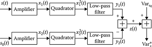
FIGURE 13.9 Flowchart of the stochastic process variance measurer.

where

υ₁(t) and υ₂(t) are the realizations of. Gaussian stationary stochastic processes describing the random variations β₁(t) and β₂(t) relative to the amplification coefficient value at the first and second channels of signal amplifer
n₁(t) and n₂(t) are the realizations of signal amplifer noise at the first and second channels
s(t) and s₀(t) are the investigated stochastic process and the reference signal, respectively

Let the reference signal be the stationary Gaussian stochastic process with the variance Var_s₀. The signal at the subtractor output takes the following form:

$z (t) = \frac{1}{T} {\int^{}}_{0}^{T} [x_{1}^{2} (t) - x_{2}^{2} (t)] d t . (13.181)$

The variance estimate is determined in the following form:

${Var}_{s}^{*} (t) = z (t) + {Var}_{s_{0}} . (13.182)$

Define the mathematical expectation and the variance of the variance estimate under assumptions made earlier

${\begin{array}{l} 〈 β_{1}^{2} (t) 〉 = 〈 β_{2}^{2} (t) 〉 = {Var}_{β}; \\ 〈 n_{1}^{2} (t) 〉 = 〈 n_{2}^{2} (t) 〉 = {Var}_{n} . \end{array} (13.183)$

The mathematical expectation of variance estimate can be presented in the following form:

$〈 {Var}_{s}^{*} 〉 = 〈 z 〉 + {Var}_{s_{0}} = (1 + {Var}_{β}) ({Var}_{s} - {Var}_{s_{0}}) + {Var}_{s_{0}} . (13.184)$

As we can see from (13.184), the bias of variance estimate can be presented in the following form:

$b {{Var}_{s}^{*}} = {Var}_{β} ({Var}_{s} - {Var}_{s_{0}}) . (13.185)$

If the variance of the reference stochastic process is controlled then the variance measurement process can be reduced to zero signal aspects at the output indicator. This procedure is called the method with zero instant. Naturally, the variance estimate is unbiased.

The variance of the variance estimate can be presented in the following form:

$\begin{array}{l} Var {{Var}_{s}^{*}} = & \frac{4 {Var}_{β}}{T} {\int^{}}_{0}^{T} (1 - \frac{τ}{T}) r_{β} (τ) [2 + r_{β} (τ) {Var}_{β}] \\ \times {{({Var}_{s} + {Var}_{n})}^{2} + {({Var}_{s_{0}} + {Var}_{n})}^{2} + 2 {{[R_{s} (τ) + R_{n} (τ)]}^{2} + {[R_{s_{0}} (τ) + R_{n} (τ)]}^{2}}} d τ \\ + {(1 + {Var}_{β})}^{2} \frac{4}{T} {\int^{}}_{0}^{T} (1 - \frac{τ}{T}) {{[R_{s} (τ) + R_{n} (τ)]}^{2} + {[R_{s_{0}} (τ) + R_{n} (τ)]}^{2}} d τ . \end{array} (13.186)$

We can simplify (13.186) applied to zero measurement procedure. In doing so, owing to identity of two channels of amplifer we can think that R_s(τ) = R_s₀(τ). Taking into consideration the condition that Var_β ≪ 1 and neglecting the terms with double frequency 2ω₀, we can write

$Var {{Var}_{s}^{*}} = {(1 + q)}^{2} \frac{4 {Var}_{s}^{2}}{T} {\int^{}}_{T}^{T} (1 - \frac{τ}{T}) [r^{2} (τ) + 4 r_{β} (τ) {Var}_{β} + 4 r^{2} (τ) r_{β} (τ) {Var}_{β}] d τ . (13.187)$

By analogy with the compensation method, (13.187) allows us to obtain the time interval of observation corresponding to the sensitivity threshold. To satisfy this condition, the following equality needs to be satisfied:

$\frac{Var {{Var}_{s}^{*}}}{{Var}_{s}^{2}} = 1. (13.188)$

Comparing (13.187) with (13.162), we can see that under the considered procedure the variance of the variance estimate is twice as high as the variance of the variance estimate at the compensation method. This increase in the variance of the variance estimate is explained by the presence of the second channel, which results in an increase in the total variance of the output signal. We need to note that although there is an increase in the variance of the variance estimate for the considered procedure, the present method is a better choice compared to the compensation method if the variance of intrinsic noise of amplifer varies after compensation procedure.

Let the normalized correlation functions, as before, be described by (13.165). Then (13.187) based on the following conditions αT ≫1 and α ≫ γ can be presented in the following form:

$Var {{Var}_{s}^{*}} = {(1 + q)}^{2} \frac{2 {Var}_{s}^{2}}{α T} {1 + 8 \frac{α}{γ} {Var}_{β} \frac{γ T - 1 + \exp {- γ T}}{γ T}} . (13.189)$

In other words, the variance of the variance estimate in the case of the considered procedure of measurement is twice as high as the variance of the variance estimate given by (13.168) obtained using compensation method. This is true also when the random variations of the amplification coefficient are absent. In doing so, the time interval of observation corresponding to the sensitivity threshold increases twofold compared to the time interval of observation of the investigated stochastic process while using the compensation method to measure the variance.

Using the deterministic harmonic signal

$s_{0} (t) = A_{0} \cos (ω_{0} t + φ_{0}) (13.190)$

as a reference signal, applied to the zero measurement procedure, that, ${Var}_{s_{0}} = 0.5 A_{0}^{2}$ , and when the random variations of the amplification coefficient are absent, the variance of the variance estimate can be presented in the following form:

$Var {{Var}_{s}^{*}} = 2 {Var}_{s}^{2} (1 + 2 q + 2 q^{2}) \times \frac{1}{T} {\int^{}}_{T}^{T} (1 - \frac{τ}{T}) r^{2} (τ) d τ . (13.191)$

As applied to the exponential normalized correlation function given by (13.165), we can transform (13.191) into the following form:

$Var {{Var}_{s}^{*}} = 2 {Var}_{s}^{2} (1 + 2 q + 2 q^{2}) \frac{2 α T - 1 + \exp {- 2 α T}}{{(2 α T)}^{2}} . (13.192)$

At αT ≫ 1, we have

$Var {{Var}_{s}^{*}} \approx \frac{{Var}_{s}^{2} (1 + 2 q + 2 q^{2})}{α T} . (13.193)$

Comparing (13.193) with (13.189) at Var_β = 0, we can see that in the case of weal signals, that is, the signal-to-noise ratio is small or q ≪ 1, with the use of the harmonic signal the variance of the variance estimate is twice as less as when the wideband stochastic process is used. Otherwise, at the high signal-to-noise ratio, q > 1, under the use of the harmonic signal the variance of the variance estimate can be higher compared to the case when we use the stochastic process. This phenomenon is explained by the presence of uncompensated components of the output signal formed by the terms of high order under expansion of the amplifer noise in series. In addition, the considered procedure possesses the errors caused by the nonidentity of channels and presence of statistical dependence between amplifer channels.

13.5.3 CORRELATION METHOD OF VARIANCE MEASUREMENT

While using the correlation method to measure the stochastic process variance, the stochastic process comes in at the inputs of two channels of amplifer. The intrinsic amplifer channel noise samples are independent of each other. Because of this, their mutual correlation functions are zero and the mutual correlation function of the investigated stochastic process is not equal to zero and the coincidence instants are equal to the variance of the investigated stochastic process. A flowchart of the variance measurement made using the correlation method is presented in Figure 13.10.

Let the independent channels of amplifer operate at the same frequency. Then the stochastic processes forming at the amplifer outputs can come in at the mixer inputs directly. We assume, as before, that the integrator is the ideal, that is, h(t) = T⁻¹. The signal at the integrator output defines the variance estimate

${Var}_{s}^{*} = \frac{1}{T} {\int^{}}_{0}^{T} x_{1} (t) x_{2} (t) d t, (13.194)$

where

${\begin{matrix} x_{1} (t) = [1 + υ_{1} (t)] [s (t) + n_{1} (t)]; \\ x_{2} (t) = [1 + υ_{2} (t)] [s (t) + n_{2} (t)] \end{matrix} (13.195)$

Images

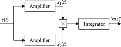
FIGURE 13.10 Correlation method of variance measurement.

are the realizations of stochastic processes at the outputs of the first and second channels, respectively. The mathematical expectation of estimate can be presented in the following form:

$〈 {Var}_{x}^{*} 〉 = \frac{1}{T} {\int^{}}_{0}^{T} 〈 s^{2} (t) 〉 d t = {Var}_{s}; (13.196)$

that is, the variance estimate is unbiased under the correlation method of variance measurement and when the identical channels are independent.

The variance of the output signal or the variance of the variance estimate of the input stochastic process in the case when the input stochastic process is Gaussian takes the following form:

$\begin{array}{l} Var {{Var}_{s}^{*}} = & \frac{2 {Var}_{s}^{2}}{T} {\int^{}}_{0}^{T} (1 - \frac{τ}{T}) [R_{β_{1}} (τ) + R_{β_{2}} (τ) + R_{β_{1}} (τ) R_{β_{2}} (τ)] d τ \\ + \frac{2}{T} {\int^{}}_{0}^{T} (1 - \frac{τ}{T}) [1 + R_{β_{1}} (τ) + R_{β_{2}} (τ) + R_{β_{1}} (τ) R_{β_{2}} (τ)] \\ \times [2 R_{s}^{2} (τ) + R_{n_{1}} (τ) R_{s} (τ) + R_{n_{2}} (τ) R_{s} (τ) + R_{n_{1}} (τ) R_{n_{2}} (τ)] d τ, \end{array} (13.197)$

where R_β1(τ) and R_β2(τ) are the correlation functions of random components of the amplification coefficients of the first and second channels of amplifier.

We can simplify (13.197) taking into consideration that the correlation interval of random components of amplification coefficients is longer compared to the correlation interval of the intrinsic noise n₁(t) and n₂(t) and the investigated stochastic process ς(t). At the same time, we can introduce the function R_β(0) = Var_β instead of the correlation function R_β(τ) in (13.197). Then, taking into consideration the condition accepted before, that is, Var_β < 1 or ${Var}_{β}^{2} ≪ 1$ , identity of channels, and (13.153) through (13.155), we obtain

$Var {{Var}_{s}^{*}} = \frac{2 {Var}_{s}^{2}}{T} (1 + q + 0.5 q^{2}) {\int^{}}_{0}^{T} (1 - \frac{τ}{T}) r^{2} (τ) d τ + \frac{4 {Var}_{s}^{2} {Var}_{β}}{T} {\int^{}}_{0}^{T} (1 - \frac{τ}{T}) r_{β} (τ) d τ . (13.198)$

Formula (13.198) allows us to define the time interval of observation T corresponding to the sensitivity threshold at the condition given by (13.188). Let the normalized correlation functions r(τ) and r_β(τ) be defined by the exponents given by (13.165) and substituting into (13.198), we obtain

$Var {{Var}_{s}^{*}} = 2 {Var}_{s}^{2} (1 + q + 0.5 q^{2}) \frac{2 α T - 1 + \exp {- 2 α T}}{{(2 α T)}^{2}} + 4 {Var}_{s}^{2} {Var}_{β} \frac{γ T - 1 + \exp {- γ T}}{{(γ T)}^{2}} . (13.199)$

When the random variations of the amplification coefficients are absent and the condition T ≫ τ_cor is satisfied, the variance of the variance estimate can be presented in the following form:

$Var {{Var}_{s}^{*}} = {Var}_{s}^{2} \frac{1 + q + 0.5 q^{2}}{α T} . (13.200)$

As we can see from (13.200), it is not difficult to define the time interval of observation corresponding to the sensitivity threshold in the case of the correlation method of measurement of the stochastic process variance.

Comparing (13.198) through (13.200) and (13.162), (13.166), and (13.169), we can see that the sensitivity of the correlation method of the stochastic process variance measurement is higher compared to the compensation method sensitivity. This difference is caused by the compensation of noise components with high order while using the correlation method and by the compensation of errors caused by random variations of the amplification coefficients. However, when the channels are not identical and there is a statistical relationship between the intrinsic receiver noise and random variations of the amplification coefficients, there is an estimate bias and the variance of estimate also increases, which is undesirable.

The correlation method used for variance measurement leads to additional errors caused by the difference in the performance levels of the used mixers and the ideal mixers. As a rule, to multiply two processes, we use the following operation:

${(a + b)}^{2} - {(a - b)}^{2} = 4 a b . (13.201)$

In other words, a multiplication of two stochastic processes is reduced to quadratic transformation of sum and difference of multiplied stochastic processes and subtraction of quadratic forms. The highest error is caused by quadratic operations.

Consider briefly an effect of spurious coupling between the amplifer channels on the accuracy of measurement of the stochastic process variance. Denote the mutual correlation functions of the amplification coefficients and intrinsic noise of amplifer at the coinciding instants as

${\begin{array}{l} 〈 β_{1} (r) β_{2} (r) 〉 = R_{β_{12}}, \\ 〈 n_{1} (t) n_{2} (t) 〉 = R_{n_{12}} . \end{array} (13.202)$

As we can see from (13.195), the bias of variance estimate is defined as

$b {V a r^{*}} = {Var}_{n} (1 + R_{β_{12}}) + R_{β_{12}} {Var}_{s} . (13.203)$

Naturally, the variance of estimate increases due to the relationship between the amplifer channels. However, the spurious coupling, as a rule, is very weak and can be neglected in practice.

13.5.4 MODULATION METHOD OF VARIANCE MEASUREMENT

While using the modulation method to measure the stochastic process variance, the received realization x(t) of stochastic process is modulated at the amplifer input by the deterministic signal u(t) with audio frequency. Modulation, as a rule, is carried out by periodical connection of the investigated stochastic process to the amplifer input (see Figure 13.11) or amplifer input to the investigated stochastic processes and reference process (see Figure 13.12). After amplification and quadratic transformation, the stochastic processes come in at the mixer input, the second input of which is used by the deterministic signal u₁(t) of the same frequency of the signal u(t). The mixer output process comes in at the low-pass filter input that make smoothing or averaging of stochastic fluctuations. As a result, we obtain the variance estimate of the investigated stochastic process.

Images

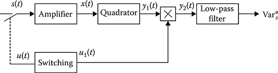
FIGURE 13.11 Modulation method of variance measurement.

Images

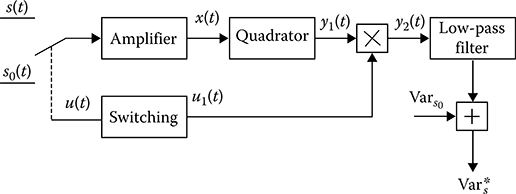
FIGURE 13.12 Modulation method of variance measurement using the reference process.

Define the characteristics of the modulation method of the stochastic process variance measurement assuming that the quadratic transformer has no inertia. The ideal integrator with the integration time T serves as the low-pass filter. Under these assumptions and conditions we can write

$u (t) = {\begin{array}{l} \begin{matrix} 1 & at & k T_{0} \leq t \leq k T_{0} + 0.5 T_{0}; \end{matrix} \\ \begin{matrix} 0 & at & k T_{0} + 0.5 T_{0} < t < (k + 1) T_{0}; \end{matrix} \\ k = 0, \pm 1, \dots; \end{array} (13.204)$

$u_{1} (t) = {\begin{array}{l} \begin{matrix} 1 & at & k T_{0} \leq t \leq k T_{0} + 0.5 T_{0}; \end{matrix} \\ \begin{matrix} - 1 & at & k T_{0} + 0.5 T_{0} < t < (k + 1) T_{0}; \end{matrix} \\ k = 0, \pm 1, \dots \end{array} (13.205)$

As we can see from (13.204), u²(t) = u(t) and the average value in time of the function u(t) can be presented as $\bar{u (t)} = 0.5$ . Analogously we have

${[1 - u (t)]}^{2} = 1 - u (t) . (13.206)$

Note that due to the orthogonality of the functions u(t) and 1 − u(t), their product is equal to zero.

At first, we consider the modulation method of the stochastic process variance measurement presented in Figure 13.11. The total realization of stochastic process coming in at the quadrator input can be presented in the following form:

$x (t) = [1 + υ (t)] {[s (t) + n (t)] u (t) + [1 - u (t)] n (t)} . (13.207)$

The process at the quadrator output takes the following form:

$y_{1} (t) = x^{2} (t) = {[1 + υ (t)]}^{2} {{[s (t) + n (t)]}^{2} u (t) + [1 - u (t)] n^{2} (t)} . (13.208)$

The process at the mixer output takes the following form:

$y_{2} (t) = {[1 + υ (t)]}^{2} {{[s (t) + n (t)]}^{2} u (t) - [1 - u (t)] n^{2} (t)} . (13.209)$

The signal at the ideal integrator output (the variance estimate) takes the following form:

${Var}_{s}^{*} = \frac{2}{T} {\int^{}}_{0}^{T} {[1 + υ (t)]}^{2} {{[s (t) + n (t)]}^{2} u (t) - [1 - u (t)] n^{2} (t)} d t . (13.210)$

The factor 2 before the integral is not important, in principle, but it allows us, as we can see later, to obtain the unbiased variance estimate and the variance of the variance estimate that are convenient to compare with the variance of the variance estimates obtained by other procedures and methods.

By averaging the random estimate ${Var}_{s}^{*}$ , we obtain

$〈 {Var}_{s}^{*} 〉 = {Var}_{s} (1 + {Var}_{β}) . (13.211)$

As we can see from (13.211), when the random variations of the amplification coefficients are absent Var_β = 0, the variance estimate of stochastic process using the modulation method of variance measurement is unbiased as is the case with the compensation method. To determine the variance of the variance estimate we need to present the function u(t) by the Fourier series expansion

$u (t) = \frac{1}{2} + \frac{2}{π} {\sum^{}}_{k = 1}^{\infty} \frac{\sin (2 k - 1) Ω t}{2 k - 1}, (13.212)$

where

$Ω = \frac{2 π}{T_{0}} (13.213)$

is the switching function frequency.

Ignoring oscillating terms and taking into consideration that Var_β ≪ 1 and the correlation interval of random component of the amplification coefficients is much more the correlation interval of the investigated stochastic process, the variance of the variance estimate, can be presented in the following form:

$\begin{array}{l} \begin{array}{l} Var {{Var}_{s}^{*}} = & \frac{32}{π^{2} T} {\sum^{}}_{k = 1}^{\infty} \frac{1}{{(2 k - 1)}^{2}} {\int^{}}_{0}^{T} (1 - \frac{τ}{T}) \\ \times {[R_{s}^{2} (τ) + 2 R_{s} (τ) R_{n} (τ) + 4 R_{n}^{2} (τ)] + 2 R_{β} (τ) ({Var}_{s}^{2} + 4 {Var}_{s} {Var}_{n} + 4 {Var}_{n}^{2})} \\ \times \cos [(2 k - 1) Ω τ] d τ + \frac{4}{T} {\int^{}}_{0}^{T} (1 - \frac{τ}{T}) [R_{s}^{2} (τ) + 2 R_{s} (τ) R_{n} (τ) + 2 R_{β} (τ) {Var}_{s}^{2}] d τ \end{array} \end{array} (13.214)$

Taking into consideration (13.153) through (13.155), (13.214) can be written in the following form:

$\begin{array}{l} Var {{Var}_{s}^{*}} = & \frac{16 {Var}_{s}^{2}}{π^{2} T} {\sum^{}}_{k = 1}^{\infty} \frac{1}{{(2 k - 1)}^{2}} \\ \times {\int^{}}_{T}^{0} (1 - \frac{τ}{T}) [(1 + 2 q + 4 q^{2}) r^{2} (τ) + 4 {Var}_{β} r_{β} (τ) (1 + 4 q + 4 q^{2})] \cos [(2 k - 1) Ω τ] d τ \\ + \frac{2 {Var}_{s}^{2}}{T} {\int^{}}_{0}^{T} (1 - \frac{τ}{T}) [(1 + 2 q) r^{2} (τ) + 4 {Var}_{β} r_{β} (τ)] d τ . \end{array} (13.215)$

In practice, the correlation interval of the investigated stochastic process is much less than the modulation period T₀ and, consequently, the time interval T of observation, since in real applications, the effective spectrum bandwidth of the investigated stochastic process is more than 10⁴ − 10⁵ Hz and at the same time, the modulation frequency f_mod = Ω × (2π)⁻¹ is several hundred hertz. In this case, we can assume that the functions cos[(2k − 1)Ωτ] are not variable functions within the limits of the correlation interval, and we can think that this function can be approximated by unit, that is, cos[(2k − 1)Ωτ] ≈ 1. This statement is true for the components of variance of the variance estimate caused by stochastic character of variation of the processes s(t) and n(t). Taking into consideration that

${\sum^{}}_{k = 1}^{\infty} {(2 k - 1)}^{- 2} = \frac{π^{2}}{8}, (13.216)$

we obtain

$\begin{array}{l} Var {{Var}_{x}^{*}} = & \frac{4 {Var}_{s}^{2}}{T} (1 + 2 q + 2 q^{2}) {\int^{}}_{0}^{\infty} r^{2} (τ) d τ + \frac{8 {Var}_{s}^{2} {Var}_{β}}{T} \\ \times {{\int^{}}_{0}^{T} (1 - \frac{τ}{T}) r_{β} (τ) d τ + \frac{8 (1 + 4 q + 4 q^{2})}{π^{2}} {\sum^{}}_{k = 1}^{\infty} \frac{1}{{(2 k - 1)}^{2}} \\ \times {\int^{}}_{0}^{T} (1 - \frac{τ}{T}) r_{β} (τ) \cos [(2 k - 1) Ω τ] d τ} . \end{array} (13.217)$

The approximation cos[(2k − 1)Ωτ] ≈ 1 is true within the limits of the correlation interval of investigated stochastic process owing to fast convergence of the series (13.216) to its limit. If, in addition to the aforementioned condition, the correlation interval of the amplification coefficients is much less than the time interval of observation, that is, τ_β ≪ 1 but τ_β > T₀, then

$Var {{Var}_{s}^{*}} \approx \frac{4 {Var}_{s}^{2}}{T} (1 + 2 q + 2 q^{2}) {\int^{}}_{0}^{\infty} r^{2} (τ) d τ + \frac{8 {Var}_{s}^{2} {Var}_{β}}{T} {\int^{}}_{0}^{\infty} r_{β} (τ) d τ . (13.218)$

When the random variations of the amplification coefficients are absent, based on (13.217), we can write

${Var}_{0} {{Var}_{s}^{*}} = \frac{4 {Var}_{s}^{2}}{T} (1 + 2 q + 2 q^{2}) {\int^{}}_{0}^{\infty} r^{2} (τ) d τ . (13.219)$

Comparing (13.219) and (13.162) at Var_β = 0 while using the compensation method to measure variance, we can see that the relative value of the variance of the variance estimate defining the sensitivity of the modulation method is twice as high compared to the relative variation in the variance estimate obtained by the compensation method at the same conditions of measurement. Physically this phenomenon is caused by a twofold decrease in the time interval of observation of the investigated stochastic process owing to switching.

Now, consider the modulation method used for variance measurement based on a comparison between the variance Var_s of the observed stochastic process ζ(t) within the limits of amplifer bandwidth and the variance Var_s₀ of the reference calibrated stochastic process s₀(t) in accordance with the block diagram shown in Figure 13.12. In this case, the signal at the amplifer input can be presented in the following form:

$x (t) = [1 + υ (t)] {[s (t) + n (t)] u (t) + [s_{0} (t) + n (t)] [1 - u (t)]} (13.220)$

The signal at the ideal integrator output can be presented in the following form:

$z (t) = \frac{2}{T} {\int^{}}_{0}^{T} {[1 + υ (t)]}^{2} {{[s (t) + n (t)]}^{2} u (t) - {[s_{0} (t) + n (t)]}^{2} [1 - u (t)]} d t . (13.221)$

The variance estimate is given by

${Var}_{s}^{*} = z + {Var}_{s_{0}} . (13.222)$

Averaging by realizations, we have

$〈 {Var}_{s}^{*} 〉 = (1 + {Var}_{β}) ({Var}_{s} - {Var}_{s_{0}}) + {Var}_{s_{0}}; (13.223)$

that is, the bias of variance estimate can be presented in the following form:

$b {{Var}_{s}^{*}} = {Var}_{β} ({Var}_{s} - {Var}_{s_{0}}) . (13.224)$

When the random variations of the amplification coefficients are absent, the process at the modulation measurer output can be calibrated in values of difference between the variance of investigated stochastic process and the variance of reference stochastic process. This measurement method is called the modulation method of variance measurement with direct reading. When the variances of investigated and reference stochastic processes are the same, the bias of the considered variance estimate is zero. If the variance of the reference stochastic process can be controlled, the measurement is reduced to fixation of zero readings. This method is called the modulation method of measurement with zero reading. The modulation method with zero reading can be automated by a tracking device.

Determine the variation in the variance estimate of the modulation method assuming as before that Var_β ≪ 1 and neglecting oscillating terms under integration and taking into consideration that τ_cor ≪ τ_β. In this case, the variance of the variance estimate of the investigated stochastic process can be presented in the following form:

$\begin{array}{l} Var {{Var}_{x}^{*}} = & \frac{32}{π^{2} T} {\sum^{}}_{k = 1}^{\infty} \frac{1}{{(2 k - 1)}^{2}} \\ \times {\int^{}}_{0}^{T} (1 - \frac{τ}{T}) [R_{s_{0}}^{2} (τ) + R_{s}^{2} (τ) + 2 R_{s} (τ) R_{n} (τ) + 2 R_{s_{0}} (τ) R_{n} (τ) + 4 R_{n}^{2} (τ)] \cos [(2 k - 1) Ω τ] d τ \\ + \frac{64}{π^{2} T} [{Var}_{s_{0}}^{2} + {Var}_{s}^{2} + 2 {Var}_{s_{0}} {Var}_{n} + 4 {Var}_{s_{0}} {Var}_{n} + 4 {Var}_{s} {Var}_{n} + 4 {Var}_{n}^{2}] \\ \times {\sum^{}}_{k = 1}^{\infty} \frac{1}{{(2 k - 1)}^{2}} {\int^{}}_{0}^{T} (1 - \frac{τ}{T}) R_{β} (τ) \cos [(2 k - 1) Ω τ] d τ \\ + \frac{4}{T} {\int^{}}_{0}^{T} (1 - \frac{τ}{T}) [R_{s}^{2} (τ) + 2 R_{s} (τ) R_{n} (τ) + R_{s_{0}}^{2} (τ) + 2 R_{s_{0}} (τ) R_{n} (τ)] d τ \\ + \frac{8}{T} {({Var}_{s} - {Var}_{s_{0}})}^{2} {\int^{}}_{0}^{T} (1 - \frac{τ}{T}) R_{β} (τ) d τ . \end{array} (13.225)$

As applied to the zero method of variance measurement, we have

$R_{s} (τ) = R_{s_{0}} (τ) = r (τ) {Var}_{s} \cos ω_{0} τ . (13.226)$

Taking into consideration (13.226), we obtain

$\begin{array}{l} Var {{Var}_{s}^{*}} = & \frac{32 {Var}_{s}^{2}}{π^{2} T} (1 + 2 q + 2 q^{2}) {\sum^{}}_{k = 1}^{\infty} \frac{1}{{(2 k - 1)}^{2}} {\int^{}}_{0}^{T} (1 - \frac{τ}{T}) r^{2} (τ) \cos [(2 k - 1) Ω τ] d τ \\ + \frac{128 {Var}_{s}^{2} {Var}_{β}}{π^{2} T} (1 + q^{2}) {\sum^{}}_{k = 1}^{\infty} \frac{1}{{(2 k - 1)}^{2}} {\int^{}}_{0}^{T} (1 - \frac{τ}{T}) r_{β} (τ) \cos [(2 k - 1) Ω τ] d τ \\ + \frac{4 {Var}_{s}^{2} (1 + 2 q)}{T} {\int^{}}_{0}^{T} (1 - \frac{τ}{T}) r^{2} (τ) d τ . \end{array} (13.227)$

In the considered case, τ_cor ≪ τ_β and τ_cor ≪ T₀, we have

$\begin{array}{l} Var {{Var}_{s}^{*}} = & \frac{8 {Var}_{s}^{2} {(1 + q)}^{2}}{T} {\int^{}}_{0}^{T} (1 - \frac{τ}{T}) r^{2} (τ) d τ \\ + \frac{256 {Var}_{s}^{2} {Var}_{β}}{π^{2} T} (1 + q^{2}) {\sum^{}}_{k = 1}^{\infty} \frac{1}{{(2 k - 1)}^{2}} {\int^{}}_{0}^{T} (1 - \frac{τ}{T}) r_{β} (τ) \cos [(2 k - 1) Ω τ] d τ . \end{array} (13.228)$

If, in addition to the foregoing statements, the random variations of the amplification coefficients are absent or the conditions τ_β ≪ T and τ_β ≫ T₀ are satisfied, we can write

${Var}_{0} {{Var}_{s}^{*}} \approx \frac{8 {Var}_{s}^{2} {(1 + q)}^{2}}{T} {\int^{}}_{0}^{T} r^{2} (τ) d τ . (13.229)$

Comparing (13.229) and (13.162) at Var_β = 0 in the case of compensation method, we can see that due to the twofold decrease in the total time interval of observation of investigated stochastic process and presence of the reference stochastic process, the variance of the variance estimate under the modulation method is four times higher compared to the variance of the variance estimate measured via the compensation method at the same conditions of measurement.

When we use the deterministic harmonic signal

$s_{0} (t) = A_{0} \cos (ω_{0} t + φ_{0}) (13.230)$

as the reference signal, we are able to obtain the variance of the variance estimate analogously. As applied to the modulation method of variance measurement with zero reading in the case of absence of the random variations of the amplification coefficients, the stochastic process variance estimate is unbiased and the variance of the variance estimate can be presented in the following form:

$Var {{Var}_{s}^{*}} = \frac{4 {Var}_{s}^{2} (1 + 2 q + 2 q^{2})}{T} {\int^{}}_{0}^{T} (1 - \frac{τ}{T}) r^{2} (τ) d τ . (13.231)$

Comparison between (13.231) and (13.191) shows us that due to a twofold decrease in the total time interval of observation, the variation in the variance estimate obtained via the modulation method measurement is twice as high compared to the compensation method.

13.6 Summary and Discussion

We summarize briefly the main results discussed in this chapter.

As we can see from (13.12), the variance of the optimal variance estimate is independent of the values of the normalized correlation function between the samples of observed stochastic process. This fact may lead to some results that are difficult to explain from the physical viewpoint or cannot be explained absolutely. As a matter of fact, by increasing the number of samples within the limits of the finite small time interval, we can obtain the estimate of variance with infinitely small estimate variance according to (13.12). The variance of optimal variance estimate of Gaussian stochastic process approaching zero is especially evident while moving from discrete to continuous observation of stochastic process.

The optimal variance estimate of. Gaussian stochastic process based on a discrete sample is equivalent to the error given by (13.24) for the same sample size (the number of samples). This can be explained by the fact that under the optimal signal processing, the initial sample multiplies with the newly formed uncorrelated sample. However, if the normalized correlation function is unknown or known with error, then the optimal variance estimate of the stochastic process has the finite variance depending on the true value of the normalized correlation function. To simplify consideration and investigation of this problem, we need to compute the variance of the variance estimate of Gaussian stochastic process with zero mean by two samples applied to the estimate by the likelihood function maximum for the following cases: The normalized correlation function, or, as it is often called, the correlation coefficient, is completely known, unknown, and known with error.

Experimental statistical characteristics of the variance estimate obtained with sufficiently high accuracy are matched with theoretical values. The maximal relative errors of definition of the math-ematical expectation estimate and the variance estimate do not exceed 1% and 2.5%, respectively Table 13.1 presents the experimental data of the mathematical expectations and variance of the variance estimate at various values of the correlation coefficient.ρ₀.between samples. Also, the theoretical data of the variation in the variance estimate based on the algorithm given by (13.24) and determined in accordance with the formula (13.40) are presented for comparison in Table 13.1. Theoretical value of the variance of the optimal variance estimate is equal to Var{Var_E} = 7.756, according to (13.5). Thus, the experimental data prove the previously discussed theoretical definition of estimates and their characteristics, at least at N = 2.

Difference between the transform characteristic and the square-law function can lead to high errors under definition of the stochastic process variance. Because of this, while using measurers to define the stochastic process variance, we need to pay serious attention to the transform performance. Verification of the transform performance is carried out, as a rule, by sending the harmonic signal of known amplitude at the measurer input. The methods discussed thus far that measure the variance assume an absence of limitations of instantaneous values of the investigated stochastic process. The presence of these limitations leads to additional errors while measuring the variance. The ideal integrator h(t) = T⁻¹ plays the role of averaging or smoothing filter.

In the majority of cases, we need to define the variance estimate by investigating a single realization of stochastic process. For measuring the variance varying in time based on a single realization of stochastic process there are similar problems as in the course of estimation of the mathematical expectation varying in time. Actually, on one hand, to decrease the variance estimate caused by the finite observation time interval, the last must be as soon as large. On the other hand, there is a need to choose an integration time as short as possible for the best definition of variance variations. Evidently, there must be a compromise.

The simplest way to define the variance of time-varying stochastic process at the instant t₀ is averaging the transformed input data of stochastic process within the limits of finite time interval. Thus, let x(t) be the realization of stochastic process ξ(t) with zero mathematical expectation. Measurement of variance of this stochastic process at the instant t₀ is carried out by averaging ordinate quadrature ordinates x(t) within the limits of the interval about the given value of argument [t₀ − 0.5T, t₀ + 0.5T]. In this case, the variance estimate is defined by (13.106). Average of the variance estimate by realizations can be defined by (13.307). Thus, as in the case of time-varying math-ematical expectation, the mathematical expectation of the estimate of the variance varying in time does not coincide with its true value in a general case, but it is obtained by smoothing the variance within the limits of finite time interval [t₀ − 0.5T, t₀ + 0.5T]. As a result of such averaging, the bias of variance of stochastic process can be presented by (13.108).

Comparing (13.187) with (13.162), we can see that in the case of comparison method, the variance of the variance estimate is twice as high compared to the variance of the variance estimate obtained via compensation method. This increase in the variance of the variance estimate is explained by the presence of the second channel because of which there is an increase in the total variance of the out-put signal. We need to note that although there is an increase in the variance of the variance estimate for the considered procedure, the present method is a better choice compared to the compensation method if the variance of intrinsic noise of amplifer changes after compensation procedure. This is also true when the random variations of the amplification coefficient are absent. In doing so, the time interval of observation corresponding to the sensitivity threshold increases twofold compared to the time interval of observation of the investigated stochastic process while using the compensation method to measure variance.

Comparing (13.198) through (13.200) and (13.162), (13.166), and (13.169), we can see that the sensitivity of the correlation method of the stochastic process variance measurement is higher compared to the sensitivity of the compensation method. This difference is caused by the compensation of noise components with high order while using the correlation method and by the compensation of errors caused by random variations of the amplification coefficients. However, when the channels are not identical and there is a statistical relationship between the intrinsic receiver noise and random variations of the amplification coefficients there is an estimate bias and an increase in the variance of estimate, which is undesirable.

Comparing (13.219) and (13.162) at Var_β = 0 in the case of compensation method of variance measurement, we can see that the relative value of the variance of the variance estimate defining the sensitivity of the modulation method is twice as high compared to the relative variation in the variance estimate of the compensation method at the same conditions of measurement. Physically, this phenomenon is caused by a twofold decrease in the time interval of observation of the investigated stochastic process due to switching.

When the random variations of the amplification coefficients are absent, the process at the modulation measurer output can be calibrated using the values of difference between the variance of the investigated stochastic process and the variance of reference stochastic process. This measurement method is called the modulation method of variance measurement with direct reading. When the variances of the investigated and the reference stochastic processes are the same, the bias of the considered variance estimate is zero. If the variance of the reference stochastic process can be controlled, the measurement is reduced to fixation of zero readings. This method is called the modulation method of measurement with zero reading. The modulation method with zero reading can be automated by a tracking device.

Comparing (13.229) and (13.162) at Var_β = 0 in the case of compensation method of variance measurement, we can see that owing to the twofold decrease in the total time interval of observation of the investigated stochastic process and the presence of the reference stochastic process the variance of the variance estimate while using the modulation method is four times higher compared to the variance of the variance estimate of the compensation method at the same conditions of measurement.

Comparison between (13.231) and (13.191) shows us that owing to the twofold decrease in the total time interval of observation in the variance of the variance estimate while using the modulation method is two times higher compared to the compensation method.

References

1. Slepian, D. 1958. Some comments on the detection of. Gaussian signals in Gaussian noise. IRE Transactions on Information Theory, 4(2): 65–68.

2. Kay, S. 2006. Intuitive Probability and Random Processes Using MATLAB. New York: Springer Science + Business Media, LLC.

3. Vilenkin, S. Ya. 1979. Statistical Processing of Stochastic Functions Investigation Results. Moscow, Russia: Energy.

4. Vilenkin, S. Ya.Esepkina, N. A., Korolkov, D. V., and Yu N. Paryisky. 1973. Radar Telescopes and Radiometers. Moscow, Russia: Nauka.

..................Content has been hidden....................

You can't read the all page of ebook, please click here login for view all page.

Table of Contents for
Chapter 13 Estimation of Stochastic Process Variance

13 Estimation of Stochastic Process Variance

13.1 Optimal Variance Estimate of Gaussian Stochastic Process

13.2 Stochastic Process Variance Estimate Under Averaging in Time

13.3 Errors Under Stochastic Process Variance Estimate

13.4 Estimate of Time-Varying Stochastic Process Variance

13.5 Measurement of Stochastic Process Variance in Noise

13.5.1 COMPENSATION METHOD OF VARIANCE MEASUREMENT

13.5.2 METHOD OF COMPARISON

13.5.3 CORRELATION METHOD OF VARIANCE MEASUREMENT

13.5.4 MODULATION METHOD OF VARIANCE MEASUREMENT

13.6 Summary and Discussion

References

Table of Contents for Chapter 13 Estimation of Stochastic Process Variance

Create new playlist

Sign In

Sign Up

Table of Contents for
Chapter 13 Estimation of Stochastic Process Variance