Chapter 8 Design Principles of Digital Signal Processing Subsystems Employed by a Complex Radar System

Search in book...
Toggle Font Controls
Create new playlist

Name your new playlist

Playlist description (optional)
Sign In

Email address

Password

Forgot Password?

or

Continue with Facebook

Continue with Google
Sign Up

Full Name

Email address

Confirm Email Address

Password

or

Continue with Facebook

Continue with Google

At the present time, the digital signal processing subsystems employed by complex radar systems (CRSs) are used to solve various problems. We aim to consider the digital signal processing subsystems implementing the following:

Solution of the problems to accumulate and process information files in real time
Information exchange between sensors and users in the course of functional problem solution
Long-time continuous processing
Simultaneous realizations of wide-range signal processing and control problems with relative consistency in the problems solved during the exploiting period

To satisfy the listed requirements, the microprocessor subsystems are designed for each case. In this section, we discuss the main design principles, parameters, and performance of microprocessor subsystems employed by digital signal processing subsystems in a CRS.

8.1.1 SINGLE-COMPUTER SUBSYSTEM

The control microprocessor (see Figure 8.1) is the central component of single-computer subsystem with the following main constituents:

Central processor consisting of the arithmetic and logic unit (ALU) and the central control device (CCD)
Random access memory (RAM) assigned to store information (programs, intermediate and end computations) directly used at the time of digital signal processing operations
External memory (EM) assigned to store large information arrays for a long time and exchange with RAM by these arrays
Input-output (I/O) devices assigned to organize the exchange of information between RAM, control microprocessor, and other facilities
Adapters, including control console, display, and so on

In management information systems, including CRSs, a single-computer subsystem possesses some devices providing an interface between sensors and users and specific subsystems of digital signal preprocessing. In Figure 8.1, these devices are united in the same block. The control microprocessor is characterized by the total engineering data. We consider the following features of engineering data that are used only to compare the microprocessor systems between each other.

Images

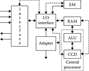
FIGURE 8.1 Control microprocessor.

Addressness: The number of address codes used by the instruction code. There are one-, two-, three-address instructions and zero-address instructions. The control microprocessor uses the one-address instructions.

Number representation capacity: The control microprocessor subsystems are characterized by 16, 24, 32, and 64 digits per word.

Number representation form: There are two number representation forms: the fixed and the floating point. The control microprocessor with the fixed point represents the numbers in the form of proper fraction, and the point is fixed before the first more significant digit (MSD). The control microprocessor with floating point represents the numbers by the sign, mantissa, and order (the normal number representation form).

Microprocessor speed of operation: To characterize the speed of operation of the microprocessor subsystem, the statement of “rated speed” is introduced independently of the solved problem class in accordance with the formula

V_{r s} = τ_{s h o r t,} (8.2)

$V_{r s} = τ_{s h o r t,} (8.2)$

where τ_short is the duration of short operation (e.g., addition).

Effective speed of operation: The average number of operations per second for obtaining the specific digital signal processing algorithm is as follows:

V_{eff} = μ \frac{N_{total}}{T_{sol}}, (8.2)

$V_{eff} = μ \frac{N_{total}}{T_{sol}}, (8.2)$

where

N_total is the total average number of operations carried out for a single realization of digital signal processing algorithm
μ is the coefficient depending on microprocessor addressness (in the case of a single-address microprocessor μ = 1)
T_sol is the time to solve the problem given by

$T_{sol} = \sum_{i = 1}^{n} N_{i} τ_{i} (8.3)$ $T_{sol} = \sum_{i = 1}^{n} N_{i} τ_{i} (8.3)$

where

n is the number of operation type, namely, addition, multiplication, division, addressing to RAM, and so on, carried out in the course of the digital signal processing algorithm
N_i is the number of the ith type operations
τ_i is the execution time of the ith type operation

Taking into consideration (8.3), we can write

V_{eff} = \frac{1}{\sum_{i = 1}^{n} ω_{i} τ_{i}} (8.4)

$V_{eff} = \frac{1}{\sum_{i = 1}^{n} ω_{i} τ_{i}} (8.4)$

where ω_i is the average execution frequency (probability) of the ith type operation.

Memory device size may be expressed in bit (memory cell), byte (8 bits), kbit (1024 bits), and kbyte. The memory device size may be expressed also using the computer word, that is, the number of words, a length of which in bits corresponds to the number representation capacity in microprocessor subsystem memory. Speed of operation of memory device is characterized by a memory device cycle time τ_cycle. Thus, the cycle time differs between recording and reading and is defined in the following form:

τ_{cycle}^{rec} = τ_{search} + τ_{rec} + τ_{clean}; (8.5)

$τ_{cycle}^{rec} = τ_{search} + τ_{rec} + τ_{clean}; (8.5)$

τ_{cycle}^{read} = τ_{search} + τ_{read} + τ_{rebuild}, (8.6)

$τ_{cycle}^{read} = τ_{search} + τ_{read} + τ_{rebuild}, (8.6)$

where

τ_search is the time required to search information
τ_rec is the time required to record information
τ_clean is the time required to clean the memory cells for preparing corresponding cells to record new information
τ_read is the time required to read information
τ_rebuild is the time required to restore information destroyed while reading

In general, the microprocessor subsystem reliability is defined by the probability of instruction issued for a correct problem solution with a single-time use of digital signal processing algorithm:

P (t_{real}) = [1 - P_{fail} (t_{real})] [1 - P_{circuit} (t_{real})], (8.7)

$P (t_{real}) = [1 - P_{fail} (t_{real})] [1 - P_{circuit} (t_{real})], (8.7)$

where

t_real is the time of a single realization of digital signal processing algorithm for the solved problem
P_fail(t_real) is the probability of microprocessor subsystem failure within the limits of t_real, which can be rebuilt without shutting down the operation of microprocessor subsystem
P_circuit(t_real) is the probability of microprocessor subsystem circuit drop-in within the limits of t_real

In the course of comparative analysis, the microprocessor subsystem’s reliability is evaluated by the average time between the microprocessor subsystem failures within the limits of t_real. Here, we understand failures associated with both the hardware and the software as the failure of microprocessor subsystem.

8.1.2 MULTICOMPUTER SUBSYSTEM

Until recently, the effective speed of operation has mainly improved due to an increase in the speed of element base operation and by designing the most efficient microprocessor subsystem functioning algorithms. At the present time, the speed of the element base operation is very close to being achieved. The use of parallel microprocessor subsystems plays a main role in increasing the effective speed of microprocessor subsystem functioning. The idea of parallel computations is very simple: several microprocessor subsystems try to solve the same problem. Technical realization of this idea depends largely on the nature of the problems to be solved (a possibility to parallel effectively a computational process) and on the level of efficacy of the modern parallel microprocessor subsystems.

One of the possible ways to increase the microprocessor subsystem performance and reliability during the digital signal processing in real time is to design and construct the multicomputer subsystems; these are used in CRSs to use effectively the digital signal processing algorithms. Computational process in the multicomputer subsystems is organized using new principles, namely, a parallel digital signal processing by several microprocessor subsystems. The main factors defining such a multicomputer subsystem structure are the end use, required performance, and memory size for the solution of the given problem in totality and functional reliability taking into consideration external environment and economical factors—the maximum permissible cost and energy consumption and so on.

To provide a solution for a single target problem, we need to organize the exchange of information between the microprocessor subsystems. This operation requires adequate memory size and speed of microprocessor subsystem operation and that microprocessor subsystems be combined in computer subsystem to be used in a CRS. Another aspect is the dead time, which is caused by expectation of final solutions of some problems at the previous levels of computer subsystem. These circumstances lead to a decrease in the multicomputer subsystems’ performance compared to a single-computer subsystem’s performance. However, other parameters such as the reliability and system survival are increased essentially. Thus, we have an opportunity to exploit the digital signal processing algorithms requiring larger memory size compared to a single-microprocessor subsystem, given the structural modifications of microprocessor subsystems with limited effective speed of operation and memory size.

In general, the multicomputer subsystem performance defined by the effective speed of multicomputer subsystem operation can be given by

Q_{eff} = K (M) \sum_{i = 1}^{M} V_{eff i}, (8.8)

$Q_{eff} = K (M) \sum_{i = 1}^{M} V_{eff i}, (8.8)$

where

V_{eff i} is the effective operation speed of the ith microprocessor
M is the number of microprocessors in the subsystem
K(M) < 1 is the coefficient taking into account the multicomputer subsystem operating costs depending on the number of microprocessors combined into a multicomputer subsystem

Microprocessors in the multicomputer subsystem may process the digital signal processing algorithms in off-line mode or while interacting with each other. In accordance with this statement, there are two types of multicomputer subsystems. The first type of multicomputer subsystems using only an information exchange between the autonomous microprocessors consist of, as a rule, the microprocessors of the same type. Each microprocessor in this multicomputer subsystem has the processor and RAM and interacts with other microprocessors through specific interface and information channels. An example of such multicomputer subsystem is the multiplexed multicomputer subsystem, in which M − m microprocessors are working and m microprocessors are redundant and M is the total number of microprocessors in the multicomputer subsystem. An important task of this multicomputer subsystem is to facilitate information exchange between the microprocessors. The information exchange can occur

Between RAM of microprocessors using the common jump-address fields
Between RAM of microprocessors using the standard information channels based on the “channel–channel” type adapters
Between EM devices using the standard information channels based on the total EM device control

The second type of multicomputer subsystems are assigned to increase the system performance by a simultaneous solution of independent paths of parallel digital signal processing algorithm. These subsystems possess programmable structure. As a rule, the second type of multicomputer subsystems consist of the same type microprocessors or they are homogeneous. Regularized programmable communication channels that are organized using the standard information channels and switchboards carry out functional interaction between microprocessors. The switchboard and the microprocessor with a block of subsystem operation realizations (BSOR) represent the elementary cell of the homogeneous multicomputer subsystem [1–3]. Combining elementary cells in the multicomputer subsystem can be carried out by ring coupling or by routing switching. One example of the ring coupling homogeneous multicomputer subsystem is shown in Figure 8.2. Switchboards S_i consist of gates opening or closing the communication channel running to a neighbor cell at the right side. BSOR consists of the adjustment register and block realizing the subsystem operations. The adjustment register content defines the switchboard function type and the degree of participation of the corresponding elementary cell while carrying out some instructions in accordance with the digital signal processing algorithm at each step. The homogeneous multicomputer subsystem operations are as follows:

Adjustment operation assigned to program a structure of connections between the elementary cells
Operation of information exchange assigned to organize the information exchange between the elementary cells of multicomputer subsystem
Operation of generalized conditional jump to control a computation process during joint functioning of microprocessors in the multicomputer subsystem
Operation of generalized unconditional jump to provide a hyphenation of computational data from one cell to other cells of the homogeneous multicomputer subsystem

Images

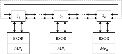
FIGURE 8.2 Ring coupling homogeneous multimicroprocessor subsystem.

The homogeneous multicomputer subsystem constructed based on these principles allows us to realize any digital signal processing algorithms. In other words, this is a universal subsystem in algorithmic sense. These homogeneous multicomputer subsystems do not have any limitations in the performance of computing complex digital signal processing algorithms and allow us to ensure the required reliability and subsystem survival in case there are unlimited number of elementary cells(microprocessors). A main task with designing homogeneous multicomputer subsystems isto define the number of elementary cells, which ensures the realization of complex digital signal processing algorithms in real time and required operational reliability taking into consideration the multicomputer subsystem losses in the effective speed of operations.

8.1.3 MULTIMICROPROCESSOR SUBSYSTEMS FOR DIGITAL SIGNAL PROCESSING

Computer subsystem consisting of several microprocessors coupled with each other by the common RAM and interface is called the multimicroprocessor subsystem. As a rule, the multimicroprocessor subsystem is designed based on the homogeneous single-microprocessor subsystems. Homogeneity ensures their interchangeability that allows us to increase efficiently the reliability and survival of the multimicroprocessor subsystem. The presence of common RAM that is equally available for all microprocessors reduces costs of the multimicroprocessor subsystem, which are required for data exchange in the course of parallel computation. The multimicroprocessor subsystem performance increases compared to the single-microprocessor subsystem due to simultaneous digital signal processing of several problems or parallel digital signal processing of some parts of the same problem. To use effectively the multimicroprocessor subsystem we need to separate a whole set of problems that must be solved on a set of subprograms that can be used in parallel and, in this case, the information delivered from the same RAM. In this case, a computational ganging is carried out by the unified control instruction stream for all microprocessors compared to the multicomputer subsystems. The multimicroprocessor subsystem programming differs from the multicomputer subsystem one and is a specific problem associated with systems programming theory and technique.

Images

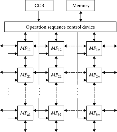
FIGURE 8.3 Matrix homogeneous multimicroprocessor subsystem.

At the present time, the homogeneous multimicroprocessor subsystems for digital signal processing are designed based on two structural types: in the case of parallel digital signal processing—the matrix and associative structure, and in the case of sequential digital signal processing—the backbone structure. The matrix of homogeneous multimicroprocessor subsystems possess a single control block (CB) and a set of microprocessors combined into a matrix form (see Figure 8.3). Each microprocessor has its own RAM and operates with internal data, and the multimicroprocessor subsystem operates with larger arrayed data. There are the central control block (CCB) and memory device that store the data and programs in the homogeneous multimicroprocessor subsystem structure. In addition, the common memory may be included in the homogeneous multimicroprocessor subsystem structure and all microprocessors are able to address the common memory following the assigned regulations. Description of the matrix homogeneous multimicroprocessor systems is widely presented in literature [4–8]. Associative parallel homogeneous multimicroprocessor subsystems differ from the matrix ones by the presence of the so-called associative memory, that is, the memory where the data are selected based on the data content, not data address. The homogeneous multimicroprocessor subsystems with parallel structure are assigned to solve the problems possessing a natural parallelism [9] since all microprocessors of this system carry out the same operation simultaneously (each microprocessor uses its own data). These subsystems can be used in CRSs used for digital signal processing operations, including spatial-time signal processing, filtering of the target trajectory parameters by recurrent filters realized in the matrix form, and others where the linear algebra operations must be done, for example, the multiplication of vectors and matrices, the matrix inversion, and so on.

The backbone multimicroprocessor subsystem combines several independent microprocessors coupled with each other in such a way that information at the output of one microprocessor comes in at the input of another microprocessor; that is, the microprocessors process information sequentially or in conveyer style. The conveyer style of digital signal processing is based on partition of the digital signal processing algorithm on a set of steps and matching in time these steps when the digital signal processing algorithm is accomplished Advantages with implementing the backbone multimicroprocessor subsystems compared to the matrix homogeneous multimicroprocessor ones are the moderate requirements with respect to inner coupling and the simplicity with which the backbone multimicroprocessor subsystem’s computational power can be increased. Further dis-advantages are removed by organizing priority exchange of information between the system cells.

Images

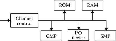
FIGURE 8.4 Backbone multimicroprocessor subsystem with a single inner long-distance channel.

Images

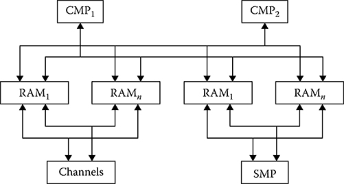
FIGURE 8.5 Backbone multimicroprocessor subsystem with multidimensional inner long-distance channel.

Two types of backbone multimicroprocessor subsystems are widely used for digital signal processing in real time [10–12]: The first type is a one-dimensional inner long-distance channel operating in the time-sharing mode (see Figure 8.4), and the second type is a multidimensional inner long-distance channel coupled with two-input RAM, in particular (see Figure 8.5). In the backbone multimicroprocessor subsystem of the first kind, all RAM and read-only memory (ROM), central microprocessor (CMP), and specific microprocessors (SMPs) are coupled by the same channel. There is a block to control the channel. This block is used in the case of conflicts when several microprocessors address RAM simultaneously and for controlling data upload and extraction using the channel units to exchange data. Operation of a single backbone multimicroprocessor subsystem is carried out in the following way. Each microprocessor submits, as needed, an application to the channel to address to RAM or ROM. If the channel is free then the microprocessor can access RAM or ROM immediately. Otherwise, the microprocessor is in the idle mode. The microprocessor can access RAM or ROM when the previous queries from other microprocessors are ended and there is no query from the microprocessors with high priority. Consequently, there are high requirements of the information channel with respect to the data throughput. Determination of the required throughput is carried out for each specific case, using the queuing theory methods. Note that the mentioned structure of the backbone multimicroprocessor subsystem has a limited speed of operation defined by the data channel throughput and, in addition, with the data channel failure the backbone multimicroprocessor subsystem stops any operation. A great advantage of the backbone multimicroprocessor subsystem is its simplicity.

In the backbone multimicroprocessor subsystem with the multidimensional inner long-distance channel (see Figure 8.5) all microprocessors operate using the independent asynchronous mode and all conflict situations are practically excluded. This system has high reliability and allows us to increase the performance without any limitations. Disadvantage of the backbone multimicroprocessor subsystem with the multidimensional inner long-distance channel is the high complexity caused by the multiinput RAM and ROM use. While designing the multimicroprocessor subsystem, the main problem is to provide the required performance by selecting the number of microprocessors to be included in this subsystem. With an increase in the number of microprocessors in the multimicroprocessor subsystem structure, a portion of overhead caused by a waiting time while the microprocessor addresses RAM or ROM and simultaneously addressing common tables and operational systems also causes an increase in the timetables related to supervisory routing. The total performance of multimicroprocessor subsystem is determined in the following form:

Q = M V_{eff}^{'} (1 - η), (8.9)

$Q = M V_{eff}^{'} (1 - η), (8.9)$

where

$V_{eff}^{'}$ $V_{eff}^{'}$ is the effective speed of operation of a single microprocessor
η is the coefficient of relative performance loss

Equation 8.9 allows us to define approximately the required number of microprocessors if the required total multimicroprocessor subsystem performance is defined in advance.

8.1.4 MICROPROCESSOR SUBSYSTEMS FOR DIGITAL SIGNAL PROCESSI NGIN RADAR

The microcomputer constructed based on a microprocessor possess high reliability and flexible universality; however, speed of operation is low. In this case, the required performance in the course of the digital signal processing in a CRS can be reached by multiple microcomputer systems using several microprocessors. Such computer systems are called the microprocessor systems. Any such microprocessor subsystem has a network facilitating communication between the elements of microprocessor subsystem for data exchange between the microcomputers. Configuration and level of complexity of such communications depend on digital signal processing algorithms used by CRSs, distribution of operations between the microcomputers, and the acceptable number of RAM used by one microcomputer.

For an example, consider the microprocessor subsystem block diagram presented in Figure 8.6. The main element of this microprocessor subsystem is the microcomputer consisting of the microprocessor, RAM, I/O interface, and switchboard providing communication between the microcomputer elements and other elements of the microprocessor subsystem. Total memory of the microprocessor subsystem is based on the RAM added to the microcomputer. Each microprocessor is able to address the local RAM or RAM of other microcomputers by means of the address translation controller (ATC). The process of any microprocessor addressing the microprocessor subsystem’s total memory is facilitated in such ways. Addressing mechanism is absolutely independent of RAM topology in the microprocessor subsystem. Access time is a function of distance to the addressed RAM cell. Communication of microcomputers with ATC is carried out by the one-channel data bus in the time-sharing mode. In doing so, we assume that the microprocessor will address mainly the local RAM; that is, the microprocessor will not use the data bus between microcomputers. However, to ensure the required reliability of the microprocessor subsystem and the possibility to increase it, the microcomputers are coupled into blocks consisting of 1-14 microcomputers.

Images

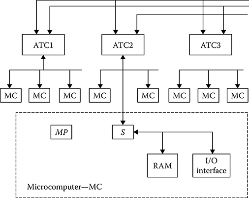
FIGURE 8.6 Example of microprocessor subsystem.

Images

FIGURE 8.7 Example of microprocessor subsystem.

The considered microprocessor subsystem structure possesses a high level of complexity of communication between the microprocessor and RAM, which leads to losses in the effective speed of operation. The high performance can be reached only when there is high efficiency of interaction between the microcomputers. In particular, the data bus overloading should be prevented. For this purpose, we need to ensure that, on priority, each microprocessor addresses local RAM in the course of the parallel digital signal processing. Another example of the microprocessor subsystem is depicted in Figure 8.7. In this microprocessor subsystem, an asynchronous communication between the microcomputers and RAM is used. If several microprocessors are coupled to the data bus they work using the time-sharing mode. Operational efficacy depends on channel throughput. For unloading the data bus, the local RAM is introduced to each microcomputer accessible for addressing by the given microprocessor. Thus, by using the data bus it is possible for other microprocessors coupled to the data bus to access the RAM. Integration of several one-channel data bus into a single data bus is possible.

8.2 Requirements for Effective Speed of Operation

Digital signal processing in CRSs is carried out in real time depending on the speed of incoming requests to realize the definite signal processing algorithms. These requests would be satisfied by a CRS within the limited time period defined by the speed of incoming requests from corresponding stages of the digital signal processing algorithms. Consequently, the main problem with designing the microprocessor subsystems is to satisfy the main limitations during attended time of requests coming into the microprocessor subsystem. A favorable basis for studying the microprocessor subsystem operation in dynamical mode, in order to define the main requirements to structure and technical parameters, is the queuing theory [13]. In this section, we define the main specifications of the microprocessor subsystems employed by CRSs with respect to the speed of operation during digital signal processing in real time.

8.2.1 MICROPROCESSOR SUBSYSTEM AS A QUEUING SYSTEM

The queuing system (QS) interacts with sources of requests for queuing. In the discussed case, the targets and other interferences in the radar coverage are considered as the sources of queuing requests (see Figure 8.8). These sources interact with the QS through the request sensor—the CRS plays this role. The radar system transforms the queuing request into signals that are subjected to process. Time sequence of these signals, which is ordered during radar sensing and scanning of the controlled space, forms an input request flux for the QS.

In general, the input request flux is considered as a stochastic process given by the probability density function of interval duration between the instants of two neighboring requests. The initial input flux of requests for a CRS is the target set in the radar coverage. At the initial designing stage, we can think that pdf of time intervals τ_tg between the neighboring targets is given by the exponential function:

p (τ_{tg}) = S_{tg} \exp {- S_{tg} τ_{tg}}, (8.10)

$p (τ_{tg}) = S_{tg} \exp {- S_{tg} τ_{tg}}, (8.10)$

Images

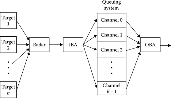
FIGURE 8.8 Radar coverage as a queuing system.

where

S_{tg} = \frac{1}{{\bar{τ}}_{tg}} (8.11)

$S_{tg} = \frac{1}{{\bar{τ}}_{tg}} (8.11)$

is the information density equal to the average number of target movements within the radar coverage along the external border per unit time; ${\bar{τ}}_{tg}$ ${\bar{τ}}_{tg}$ is the average time interval between two considered events (the target traverses). The flux with pdf of time intervals τ_tg given by (8.10) is called the Poisson flow. If additional requirements of stationarity, ordinariness, and absence of sequence are satisfied, then the Poisson flow is called the simplest Poisson flow [14–16]. The average number of targets in the radar coverage is given by

{\bar{N}}_{tg} = S_{tg} \bar{t_{rc}}, (8.12)

${\bar{N}}_{tg} = S_{tg} \bar{t_{rc}}, (8.12)$

where ${\bar{t}}_{rc}$ ${\bar{t}}_{rc}$ is the average time of target being within the limits of radar coverage. Furthermore, we assume that the targets are distributed uniformly within the limits of radar coverage with the same pdf per unit volume. At the input of a digital signal processing subsystem (the radar receiver) of a CRS, the spatial pattern of targets distribution within the limits of the radar coverage is transformed into the time sequence of signals adhering to process. Henceforth, this signal flux is considered as the simplest with the intensity

γ_{tg} = {\bar{N}}_{tg} T_{scan}, (8.13)

$γ_{tg} = {\bar{N}}_{tg} T_{scan}, (8.13)$

where T_scan is the period of radar coverage scanning.

In many cases, the hypothesis about the simplest flux of requests at the digital signal processing subsystem does not correspond to parameters and characteristics of real incoming signal flux. Nevertheless, an implementation of this hypothesis is considered acceptable for designing radar systems by the following reasons:

First, analysis of QS is very simple.
Second, because the simplest incoming signal flux is a very hard problem for such QSs, the CRS designed based on the simplest flux representation ensures successful service of other possible signal fluxes with the same intensity.

Along with the target return signals, the interferences (the false signals) caused by the internal and external noise sources come in at the input digital signal processing subsystem as requests for service. This interference (the false signals) flux can also be considered as the simplest flux with definite assumptions.

The incoming flux request service is organized by the QS. The QS can be considered as both the device carrying out a direct request service and the device assigned to store a request queue adhering to service. The QS is characterized by (see Figure 8.8) the following:

The number of devices (cells) assigned to store a request queue of the incoming signal flux (the input buffer accumulator (IBA) memory size)
The number of devices (channels) K that can serve multiple requests simultaneously
The number of devices (cells) that accumulate and store the digital signal processing results (the IBA memory size)

The request queue is stored by the microprocessor subsystem IBA. The waiting time and the number of queued requests (the request queue length) are the random variables depending on statistical parameters of the incoming signal flux and service rate. Because the IBA size (memory capacity) is limited, the request queue length and, consequently, the waiting time of request queue are limited too. This QS is called the queuing system with the limited queue (the limited waiting time). Thus, the digital signal processing subsystem can be considered as the subsystem belonging to the class of QSs with limited queue.

The request queue in the digital signal processing subsystem of a CRS is realized by the microprocessors that can belong to a single or a set of parallel channels and is reduced to a single program realization of the corresponding digital signal processing algorithms. The time requested for each realization of the digital signal processing algorithm is the random variable owing to many reasons and, consequently, can be given statistically only. If we denote the time of a single request queue as τ_queue, then the sufficient characteristic of τ_queue, as a random value, is the pdf p(τ_queue). QSs with the exponential pdf of τ_queue

p (τ_{queue}) = μ \exp {- μ τ_{quene}} (8.14)

$p (τ_{queue}) = μ \exp {- μ τ_{quene}} (8.14)$

play a specific role in the queuing theory, where

μ = \frac{1}{{\bar{τ}}_{queue}} (8.15)

$μ = \frac{1}{{\bar{τ}}_{queue}} (8.15)$

is the queue intensity. The request queue approximation by the exponential pdf in the digital signal processing subsystem of a CRS allows us to carry out an analytical estimation of statistical characteristics of the request queue process during the simplest incoming signal flux using a sufficiently easy way.

If the request queue in the digital signal processing subsystem is carried out by K identical channels or microprocessors coupled with these channels and each channel or microprocessor has the exponential pdf of τ_queue, then the pdf of τ_queue for whole digital signal processing (microprocessor) subsystem is determined in the following form:

p (τ_{queue}) = \frac{K}{{\bar{τ}}_{queue}} \times \frac{{(τ_{queue})}^{K - 1}}{(K - 1)!} \exp {- μ^{K} τ_{queue}}, (8.16)

$p (τ_{queue}) = \frac{K}{{\bar{τ}}_{queue}} \times \frac{{(τ_{queue})}^{K - 1}}{(K - 1)!} \exp {- μ^{K} τ_{queue}}, (8.16)$

where

{\bar{τ}}_{queue} = \frac{1}{μ K} (8.17)

${\bar{τ}}_{queue} = \frac{1}{μ K} (8.17)$

is the average time queue. Distribution law given by (8.16) is called the Erlang distribution (pdf). At K = 1, the Erlang distribution is transformed into exponential pdf. Other distribution laws that can be represented by some exponential functions with different decay rates are used too. Presentation of distribution laws based on combination principle of exponential components allows us to approximate the request queue by Markov process and to obtain an analytical solution of this problem. Unfortunately, in CRS digital signal processing subsystems, the pdf of τ_queuediffers from the exponential pdf and cannot be reduced to Erlang distribution law. For this reason, the pdfs of τ_queue must be analyzed for each specific case of designing the CRS digital signal processing subsystem.

Finally, let us discuss some observations about the flux forming at the digital signal processing subsystem output, that is, the output flux. At first, the output flux is stored by the output buffer accumulator (OBA). Thereafter, the output flux with the given rate is transferred to the user. As a rule, the digital signal processing of target return signals is realized by a set of serial microprocessor subsystems. In the course of the digital signal processing, we need to make transformations of fluxes; for instance, the signal flux must be transformed into the coordinate flux or the detected target pip flux that must be transformed into the flux of target tracking trajectory parameters and so on. In doing so, in the course of the digital signal processing, the output flux of the previous stage is the input flux of the next stage.

In the considered case, the output fluxes at each stage of the digital signal processing, as well as the input fluxes, can be considered as the simplest fluxes and their intensities can be determined using the estimated parameters of target and noise situations within the limits of the radar coverage. For example, the flux density of true target pips at the digital signal preprocessing subsystem output is defined by the number of targets within the limits of the radar coverage, the probability of target detection, and the scanning rate. Analogously, the flux density of false target pips is defined by the noise environment within the limits of the radar coverage, the scanning rate, and so on. Knowledge about the output fluxes is required to establish the necessary IBA size (capacity) for designing the information buses to exchange information between the microprocessors in the microprocessor subsystem and the communication channels to transfer information to the user.

8.2.2 FUNCTIONING ANALYSIS OF SINGLE-MICROPROCESSOR CONTROL SUBSYSTEM AS QUEUING SYSTEM

Images

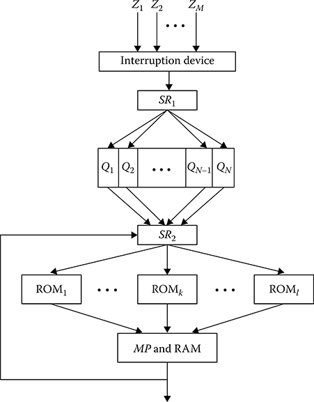
FIGURE 8.9 Single-microprocessor digital signal processing subsystem.

Assume that the digital signal processing subsystem is realized based on a single-microprocessor subsystem (see Figure 8.9). We think that the request flux comes in at the input of the digital signal processing subsystem. The request flux is the multidimensional process consisting of M components corresponding to the given number of digital signal processing algorithms assigned to be realized by a single-microprocessor subsystem. The requests z₁, z₂,…, z_M come in at the input of interruption device included into the microprocessor structure. When the request z_i comes in at the input of interruption device, this device interrupts the computation process and transfers control to the supervisory routine SR₁ that organizes the receiving process and the request z_i queue in accordance with assigned priority if this request z_i does not belong to immediate processing. The queuing process is stored by the buffer accumulator (BA). In doing so, the groups of cells Q₁, Q₂,…, Q_N form regions where the requests will be stored with corresponding priority. Within the limits of each priority zone, the requests are written on the first come first ordering basis. After receiving and queuing, the control is transferred to the supervisory routine SR₂ that organizes the digital signal processing of requests from queuing using the microprocessor.

The process of selecting a new request from a set of requests waiting in queue is the following. After the digital signal processing of immediate request, the supervisory routine SR₂ investigates sequentially queuing Q₁, Q₂, …, Q_N and selects for service the request z_k possessing the greatest priority. After initiation of the corresponding routine R_k, it is realized by the microprocessor. The queued request z_k leaves the system and the control is transferred to the supervisory routine SR₂ again. If there are no further requests, then the supervisory routine SR₂ switches on the microprocessor in the idle mode. At each instance, the microprocessor can run a single program only. For this reason, the considered QS is called a single-channel or a single-microprocessor QS.

One of the important quality parameters of the microprocessor subsystem as a QS is the capacity factor that characterizes the time interval within the limits of which the QS (microprocessor) processes a request and simultaneously the probability that the QS works (no idle mode) at the present time. The input flux with the density λ_k can be determined in the following form:

ρ_{k} = \frac{λ_{k}}{μ_{k}}, (8.18)

$ρ_{k} = \frac{λ_{k}}{μ_{k}}, (8.18)$

where

μ_{k} = \frac{1}{τ_{queue k}} (8.19)

$μ_{k} = \frac{1}{τ_{queue k}} (8.19)$

is the intensity of the request queue of the kth flux. The total loading factor of the microprocessor subsystem by all M incoming flux is defined in the following form:

U = \sum_{k = 1}^{M} ρ_{k} . (8.20)

$U = \sum_{k = 1}^{M} ρ_{k} . (8.20)$

The steady stationary operation mode of QS is the mode where the probability characteristics of QS functioning are independent of time. The condition of existence of the steady mode is defined by the loading factor U < 1. The value $Q = 1 - U$ $Q = 1 - U$ is called the downtime ratio. In the steady QS functioning mode the down ratio is positive, that is, $Q > 0$ $Q > 0$ . Logically, the value of $Q$ $Q$ facilitated by the microprocessor subsystem must be minimal. Operation quality of the microprocessor subsystem as the QS is defined by the time of request processing by the microprocessor subsystem defined from the instant of request coming in at the microprocessor subsystem until the time a service is concluded by the microprocessor subsystem. For the kth request, this time consists of the waiting time for queuing t_{wait k} and the queuing time τ_{queue k}:

{\bar{τ}}_{Σ k} = {\bar{t}}_{wait k} + {\bar{τ}}_{queue k}, (8.21)

${\bar{τ}}_{Σ k} = {\bar{t}}_{wait k} + {\bar{τ}}_{queue k}, (8.21)$

where ${\bar{t}}_{wait k}$ ${\bar{t}}_{wait k}$ and ${\bar{τ}}_{queue k}$ ${\bar{τ}}_{queue k}$ are the average values. The waiting time ${\bar{t}}_{wait k}$ ${\bar{t}}_{wait k}$ depends on the regulation applied to the request queuing—the order of multidimensional flux request selection for queuing from the total number of requests. There are the following regulations for request queuing:

Nonpriority request queuing: The queuing in the order of request coming in at the QS, that is, in other words, “who could come early, he is the first.”
Relative priority request queuing: Priority for queuing is taken into consideration only at the instant to be served.
Absolute priority: The incoming request with higher priority interrupts the queued request with lower priority.

During nonpriority request queuing, the average waiting time for all requests is the same and given by

{\bar{t}}_{wait} = \sum_{k = 1}^{M} \frac{1 + υ_{k}^{2}}{2 (1 - U)} ρ_{k} {\bar{τ}}_{queue k}, (8.22)

${\bar{t}}_{wait} = \sum_{k = 1}^{M} \frac{1 + υ_{k}^{2}}{2 (1 - U)} ρ_{k} {\bar{τ}}_{queue k}, (8.22)$

where

υ_{k} = \frac{σ_{queue k}}{{\bar{τ}}_{queue k}} (8.23)

$υ_{k} = \frac{σ_{queue k}}{{\bar{τ}}_{queue k}} (8.23)$

is the variation factor defined by the ratio between the root mean square deviations of τ_{queue k} to its average value ${\bar{τ}}_{queue k}$ ${\bar{τ}}_{queue k}$ . In accordance with (8.22), the value of ${\bar{t}}_{wait}$ ${\bar{t}}_{wait}$ will be minimum at the constant value of τ_{queue k}, that is, at υ_k = 0. In the case of exponential pdf of τ_{queue k}, υ_k = 1 and, consequently, there is a twofold increase in ${\bar{t}}_{wait}$ ${\bar{t}}_{wait}$ when υ_k = 0.

The widely used regulation in the information subsystem with the request queuing in CRSs is the regulation with the fixed relative priorities for each component of request flux. In this regulation, an appearance of the request with high priority does not interrupt the request queuing process with lower priority if it has been started. In this case, the average waiting time for the ith request independently on distribution law of τ_{queue i} is given by

{\bar{t}}_{wait i} = \sum_{k = 1}^{M} \frac{1 + υ_{k}^{2}}{2 (1 - U_{i - 1}) (1 - U_{i})} ρ_{k} {\bar{τ}}_{queue k}, (8.24)

${\bar{t}}_{wait i} = \sum_{k = 1}^{M} \frac{1 + υ_{k}^{2}}{2 (1 - U_{i - 1}) (1 - U_{i})} ρ_{k} {\bar{τ}}_{queue k}, (8.24)$

where

U_{i - 1} = ρ_{1} + ρ_{2} + \dots + ρ_{i - 1} (8.25)

$U_{i - 1} = ρ_{1} + ρ_{2} + \dots + ρ_{i - 1} (8.25)$

is the loading factor of the microprocessor subsystem created by signal fluxes with priorities higher than i; the higher priority, the lesser i;

U_{i} = ρ_{1} + ρ_{2} + \dots + ρ_{i} (8.26)

$U_{i} = ρ_{1} + ρ_{2} + \dots + ρ_{i} (8.26)$

is the loading factor created by signal fluxes with priorities not lower than i. Analysis of (8.24) shows that with a decrease in priority the waiting time to start the request queuing increases monotoni-cally. Comparing the waiting time of requests with the relative priorities with the waiting time for the nonpriority request queuing, we can see that an introduction of relative priorities leads to a decrease in the waiting time for the request queuing with high priority owing to an increase in the waiting time for the request queuing with low priorities.

Level of total loading of the microprocessor subsystems with the QSs stimulates a waiting time for the request queuing with relative priorities. If the loading level of the microprocessor subsystems with the QSs is low, that is, U = 0.2–0.3, the presence of relative priorities for the request queuing has a very small effect on the waiting time between the requests of various signal fluxes. If the loading factor is close to unit, this effect becomes more essential and leads essentially to a reduction in the waiting time for the request queuing with high priorities owing to an increase in the waiting time for request queuing with low priority. In addition to the discussed regulations of requests queuing, in some cases, the regulations of requests queuing with absolute priorities are used for some components of the signal flux. Employing the request QSs with absolute priorities, the average waiting time is defined in the following form:

{\bar{t}}_{wait i} = \frac{U_{i - 1} τ_{queue k}}{1 - U_{i - 1}} + \frac{1}{2 (1 - U_{i - 1}) (1 - U_{i})} \sum_{k = 1}^{M} (1 + υ_{k}^{2}) ρ_{k} {\bar{τ}}_{queue k} . (8.27)

${\bar{t}}_{wait i} = \frac{U_{i - 1} τ_{queue k}}{1 - U_{i - 1}} + \frac{1}{2 (1 - U_{i - 1}) (1 - U_{i})} \sum_{k = 1}^{M} (1 + υ_{k}^{2}) ρ_{k} {\bar{τ}}_{queue k} . (8.27)$

Evidently, an introduction of absolute priorities in the request QS leads to a reduction in the waiting time for the request queuing with high priorities, however with a simultaneous increase in the waiting time for the request queuing with low priorities.

Dependences illustrating the average waiting time of the request queuing as a function of priorities of the request queuing are shown in Figure 8.10. During the nonpriority request queuing (the curve 1, Figure 8.10), the average waiting time is constant. In the case of relative (the curve 2) and absolute (the curve 3) priorities, there takes place an increase in the waiting time for the high priority request queuing due to an increase in the waiting time for the low priority request queuing.

As a rule, we need to follow strong limitations with respect to the waiting time for request queuing of individual signal fluxes that require assigning them by absolute priorities, for example, the requests to process the target return signals. Other requests have excess waiting time and may be assigned with relative priorities. Several requests can be served by the simple queuing procedure. Thus, we see that we need to apply mixed regulations for request queuing, the investigation of which is carried out for each specific case by simulation procedures.

Referring to (8.21), we need to pay attention to the following fact The average waiting time ${\bar{t}}_{wait k}$ ${\bar{t}}_{wait k}$ is the constituent of the total request queuing time as well as the average request queuing time ${\bar{τ}}_{queue k}$ ${\bar{τ}}_{queue k}$ . However, the request queuing time does not vary for different regulations of the request QS. For this reason, the main time characteristic of the microprocessor subsystem operation is the average

Images

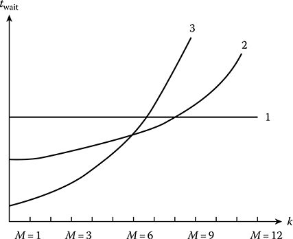
FIGURE 8.10 The average request queuing waiting time versus the request queuing priorities.

waiting time ${\bar{t}}_{wait k}$ ${\bar{t}}_{wait k}$ . Other parameters and characteristics of the request QS will be introduced as needed.

8.2.3 SPECIFICATIONS FOR EFFECTIVE SPEED OF MICROPROCESSOR SUBSYSTEM OPERATION

In the considered case, the initial data that define the specifications for effective speed of the microprocessor subsystem operation include the following:

The digital signal processing algorithm represented in the form of flow graph for each of the signal or request flux constituents
The work content of constituents of the complex computational process algorithm expressed by the average number and variance of number of operations carried out for a single realization of these algorithms
The type of the request QS of the designed microprocessor subsystem

Representation of the complex computational process algorithms and determination of the work content of these algorithms are carried out by methods discussed in Chapter 7.

The request queuing type or the type of microprocessor subsystem is defined by time requirements to process the requests by request QS or, independent of the request queuing type or the type of microprocessor subsystem, by the acceptable waiting time of the request QS. Accordingly, we call the microprocessor subsystems of the first type such microprocessor subsystems in which there are no limitations on the request queuing waiting time for all constituents of incoming signal flux. These microprocessor subsystems require the effective microprocessor operation speed that satisfies the request queuing within the finite time interval limits, the limiting value of which is unlimited in the considered case.

The request queuing waiting time is finite if the microprocessor subsystem works in the stationary mode, that is, if the total loading factor U of the microprocessor subsystem is less than the unit. The condition of stationarity takes the following form:

\sum_{k = 1}^{M} ρ_{k} = \sum_{k = 1}^{M} λ_{k} {\bar{τ}}_{queue k} < 1 . (8.28)

$\sum_{k = 1}^{M} ρ_{k} = \sum_{k = 1}^{M} λ_{k} {\bar{τ}}_{queue k} < 1 . (8.28)$

The average queuing duration ${\bar{τ}}_{queue k}$ ${\bar{τ}}_{queue k}$ is related to the work content ${\bar{N}}_{0 k}$ ${\bar{N}}_{0 k}$ and effective speed V_eff of the microprocessor subsystem operation in the following form:

{\bar{τ}}_{queue k} = \frac{N_{0 k}}{V_{eff}}, k = 1, 2, \dots, M . (8.29)

${\bar{τ}}_{queue k} = \frac{N_{0 k}}{V_{eff}}, k = 1, 2, \dots, M . (8.29)$

Substituting (8.29) into (8.28), we obtain

\begin{matrix} \frac{1}{V_{eff}} \sum_{k = 1}^{M} λ_{k} {\bar{N}}_{0 k} < 1 & or & V_{eff} > \sum_{k = 1}^{M} λ_{k} {\bar{N}}_{0 k} . \end{matrix} (8.30)

$\begin{matrix} \frac{1}{V_{eff}} \sum_{k = 1}^{M} λ_{k} {\bar{N}}_{0 k} < 1 & or & V_{eff} > \sum_{k = 1}^{M} λ_{k} {\bar{N}}_{0 k} . \end{matrix} (8.30)$

Equation 8.30 defines the minimum required speed of the microprocessor subsystem operation to establish the stationary operation mode of the microprocessor subsystem to realize the given set of digital signal processing algorithms in a CRS. If existing or assumed to be employed in the digital signal processing subsystems of CRS types of control single-microprocessor subsystems do not satisfy the main requirement given by (8.30), then the computation can be provided by the multimicroprocessor subsystems only. In this case, the parallel problem of computational process arises and we need to design the corresponding tools and facilities of parallel digital signal processing.

If the control single-microprocessor subsystem can satisfy the specifications and requirements for the effective speed of operation of the request QSs of the first type, we should study the possibilities of organizing the request QSs of the second and third types employing this control single-microprocessor systems. We call the control single-microprocessor subsystem of the second class subsystem if there are limitations on the average request queuing waiting time for all or several constituents of signal flux. The limitations are given in the following form:

{\bar{t}}_{wait k} \leq t_{k}^{*}, k = 1, 2, \dots, L, L \leq M, (8.31)

${\bar{t}}_{wait k} \leq t_{k}^{*}, k = 1, 2, \dots, L, L \leq M, (8.31)$

where $t_{k}^{*}$ $t_{k}^{*}$ is the limiting value of the average request-QS time for requests of the kth incoming signal flux.

Now, let us define the problem of the effective operation speed determination in the control single-microprocessor subsystem providing the request queuing with the given limitations and taking into consideration the fact that, similar to the request QSs of the first type, all requests are queued, with the so-called request QSs without loss and the average request queuing waiting time remaining limited. In the considered case, the minimal required speed of operation depends strongly on the request queuing regulation. If, for example, there is a nonpriority request QS, in which the average waiting time for all requests is the same and given by (8.22), the required effective speed of operation of the control single-microprocessor subsystem of the second type is determined by the following inequality:

\frac{\sum_{k = 1}^{M} λ_{k} {\bar{τ}}_{queue k} < 1 (1 + υ_{k}^{2})}{2 {1 - \sum_{k = 1}^{M} λ_{k} {\bar{τ}}_{queue k}}} \leq t^{*} . (8.32)

$\frac{\sum_{k = 1}^{M} λ_{k} {\bar{τ}}_{queue k} < 1 (1 + υ_{k}^{2})}{2 {1 - \sum_{k = 1}^{M} λ_{k} {\bar{τ}}_{queue k}}} \leq t^{*} . (8.32)$

Solution of (8.32) can be presented in the following form:

V_{eff} \geq \frac{1}{2} \sum_{k = 1}^{M} λ_{k} {\bar{N}}_{0 k} + \sqrt{0.25 {\sum_{k = 1}^{M} λ_{k} {\bar{N}}_{0 k}}^{2} + {(t^{*})}^{- 1} \sum_{k = 1}^{M} λ_{k} {\bar{N}}_{0 k} (1 + υ_{k}^{2}) .} (8.33)

$V_{eff} \geq \frac{1}{2} \sum_{k = 1}^{M} λ_{k} {\bar{N}}_{0 k} + \sqrt{0.25 {\sum_{k = 1}^{M} λ_{k} {\bar{N}}_{0 k}}^{2} + {(t^{*})}^{- 1} \sum_{k = 1}^{M} λ_{k} {\bar{N}}_{0 k} (1 + υ_{k}^{2}) .} (8.33)$

Based on (8.33), we are able to define the required speed of operation of the control single-microprocessor subsystem by the given (the same for the request queuing of all signal flux constituents) limitation on the average request QS waiting time during the nonpriority request queuing at the time of signal flux constituents coming in at the single-microprocessor subsystem input. In the limiting case, when there are no limitations in waiting time (t* → ∞), (8.33) transforms into the following form:

V_{eff} \geq \sum_{k = 1}^{M} λ_{k} {\bar{N}}_{0 k}, (8.34)

$V_{eff} \geq \sum_{k = 1}^{M} λ_{k} {\bar{N}}_{0 k}, (8.34)$

that is, it coincides with (8.30). At t* < ∞, the required effective speed of operation of the second-type control single-microprocessor subsystem is greater than that of the control single-microprocessor subsystem of the first type.

To organize the priority request queuing, for example, the relative priority, we need to take into consideration a difference in limitations applied to the average request QS waiting time of each priority in the second type of request QS. In principle, this problem can be solved by the following way. All requests are divided into groups with the same value of average waiting time. The loading factor and required effective speed of operation V_eff of the control single-microprocessor subsystem is defined for each request group. Making summation of partial values of the effective speed of operation, we obtain

V_{eff} = \sum_{p = 1}^{P} V_{eff p}, (8.35)

$V_{eff} = \sum_{p = 1}^{P} V_{eff p}, (8.35)$

where P is the number of request groups with approximately the same acceptable average waiting time of request queuing. In the considered case of the second-type request QS, as well as in the case of the first-type request QS, a decision to realize the control single-microprocessor subsystem is made as a result of comparison of requirements and specifications to effective speed of operations of the request QS with effective speed of the CMP operation. The third type of request QS is called the microprocessor subsystem that generates limitations on accept-able (absolute) time to process the request by the request QS. In these cases, the limitations are given in the following form:

P (t_{wait k} > T_{k}^{*}) \leq P *, (8.36)

$P (t_{wait k} > T_{k}^{*}) \leq P *, (8.36)$

where

$T_{k}^{*}$ $T_{k}^{*}$ is the allowed waiting time for requests of the kth signal flux
P* is the allowable probability to satisfy the inequality $t_{wait k} > T_{k}^{*}$ $t_{wait k} > T_{k}^{*}$

The request queuing waiting time probability distribution function of the total signal flux can be approximated with satisfactory accuracy by the following formula [17-19]:

P (t_{wait} \leq τ) = 1 - R \exp {- \frac{R τ}{{\bar{t}}_{wait}}} . (8.37)

$P (t_{wait} \leq τ) = 1 - R \exp {- \frac{R τ}{{\bar{t}}_{wait}}} . (8.37)$

In this case, the probability of exceeding the allowed waiting time T_k can be determined in the following form:

P (t_{wait} > T *) = 1 - R \exp {- \frac{R T *}{{\bar{t}}_{wait}}} . (8.38)

$P (t_{wait} > T *) = 1 - R \exp {- \frac{R T *}{{\bar{t}}_{wait}}} . (8.38)$

For example, in the case of the nonpriority request queuing regulation, for which ${\bar{t}}_{wait}$ ${\bar{t}}_{wait}$ is given by (8.22), based on solution of the transcendent equation we can write

1 - R \exp {- \frac{R T *}{{\bar{t}}_{wait}}} = P * (8.39)

$1 - R \exp {- \frac{R T *}{{\bar{t}}_{wait}}} = P * (8.39)$

We can obtain the required effective speed of operation of the control third-type single-microprocessor subsystem. Mathematical notation of (8.39) with respect to V_eff is tedious, and solution can be obtained only by numerical procedures.

The required effective speed down boundary definition of the third-type control single-microprocessor subsystem operation can be considered as the initial stage of designing the microprocessor subsystem for CRS digital signal processing. The next stage is a choice of the optimal request queuing regulation. At the system design stage, we will not have sufficient information to choose the specific request queuing regulation, but we should take into consideration the following circumstances:

The request queuing regulation based on request queuing in turn to come in at the control single-microprocessor subsystem possesses the best performance among all the nonpriority request queuing regulations; in particular, the variance of the request queuing waiting time is minimal compared to other nonpriority request queuing regulations.
Introduction of the priority request queuing regulation allows us to decrease essentially the request queuing waiting time for the most important requests of signal flux owing to increase in the delay during the queuing of signal minor fluxes.
In general, an introduction of the priority request queuing regulations provides an equivalent performance of the control single-microprocessor subsystem compared to the request queuing one in turn. Consequently, the determined values of the required minimum speed of the control single-microprocessor subsystem operation makes it possible to choose the priority request queuing regulation without any additional increase in the effective speed of operation.

Now, let us discuss some ways of choosing the optimal speed of operation of the control single-microprocessor subsystem. The minimum value of the effective speed of operation ensures the boundary values of the request queuing waiting time of the earlier-considered types of the request queuing regulations for the control single-microprocessor subsystem and related to a queue length that can be defined for the kth signal flux as l_k = λ_kt_{wait k}. Queue existence and its storage are related to definite losses. To decrease these losses, the effective speed of control single-microprocessor subsystem operation must be greater than the minimal one. However, in this case, the loading factor U decreases and, correspondingly, the idle time factor Q = 1 − U increases, which is not good from the point of view of hardware costs.

Evidently, we can select the optimal speed of operation taking into consideration these two contradictory factors. As the criterion of effectiveness we use the functional in the following form:

C_{V} = β_{Q} Q (V_{eff}) + \sum_{k = 1}^{M} β_{k} λ_{k} {\bar{t}}_{wait k} (V_{eff}), (8.40)

$C_{V} = β_{Q} Q (V_{eff}) + \sum_{k = 1}^{M} β_{k} λ_{k} {\bar{t}}_{wait k} (V_{eff}), (8.40)$

where

β_Q is the loss caused by idle mode
β_k, k = 1, 2, …, M are the losses caused by the queue length for each signal flux request queuing

The optimal value of the effective speed of control single-microprocessor subsystem operation can be obtained from solution of the following equation:

\frac{d C_{V}}{d V_{eff}} = 0 at \frac{d^{2} C_{V}}{d V_{eff}^{2}} > 0. (8.41)

$\frac{d C_{V}}{d V_{eff}} = 0 at \frac{d^{2} C_{V}}{d V_{eff}^{2}} > 0. (8.41)$

Solution of (8.41) is not difficult, but a choice of losses β_Q and β_k is difficult. A single acceptable procedure for this choice is the procedure of expert judgments.

8.3 Requirements for Ram Size and Structure

Requirements for RAM size and structure are defined based on the end use of system, character and digital signal processing algorithms, and an analysis of input and output signal fluxes. As a first approximation, the total RAM size (memory capacity) is defined from the formula

Q_{Σ} = Q_{routine} + Q_{digit}, (8.42)

$Q_{Σ} = Q_{routine} + Q_{digit}, (8.42)$

where

Q_routine is the RAM cell array assigned to store the routines of digital signal processing algorithms, control routine of computational process and operation of whole system, interruption routines, and routines controlling calculations
Q_digit is the RAM cell array assigned to store a numerical information

In turn, Q_digit can be presented in the following form:

Q_{digit} = Q_{in} + Q_{working} + Q_{out}, (8.43)

$Q_{digit} = Q_{in} + Q_{working} + Q_{out}, (8.43)$

where

Q_in is the RAM cell array assigned to receive external information
Q_working is the RAM cell array participating at the calculation process
Q_out is the RAM cell array assigned to store the digital signal processing results

In many cases, the relative independence of routine information on numerical one leads us to expediently use individual permanent memory or ROM to store the routine information. ROM uses only a reading mode. Implementation of ROM gives us a great advantage because information stored by ROM is not lost even if the power is off. In addition, ROM possesses high reliability. As for ROM size (capacity), at the initial stage of designing the digital signal processing subsystem it is possible to estimate this parameter approximately. The exact estimation is possible only after program debugging.

Now consider some ways of choosing the size (capacity) of memory to be assigned to store the numerical information. The cell array Q_out forms a buffer memory. The buffer memory size depends on the number of external objects, information content incoming from each object within the limits of digital signal processing cycle, microprocessor operation speed, request queuing regulation, and so on. Consider the example of the control single-microprocessor subsystem receiving information from a 3D CRS with the space periodical scanning. Assume that the number of scanned targets is ${\bar{N}}_{scan}^{tg}$ ${\bar{N}}_{scan}^{tg}$ . Information about each target at the control single-microprocessor subsystem input (the target pip) includes the spherical coordinates of the current target position and the variance of error for the measurement of these coordinates. We assume that the coordinate code width and coordinate measurement errors are established at the previous stages of digital signal processing and is characterized by the number of binary digits n_p for each target pip. Digital signal processing procedure must be organized in such a way that information obtained during the previous cycle would be completely processed during the next cycle. Thus, during the cycle equal to the scanning period, ${\bar{N}}_{scan}^{tg}$ ${\bar{N}}_{scan}^{tg}$ of n_p-digit words will be recorded in the buffer memory. If we assume that a target distribution in the radar coverage is uniform, the target pip flux at the buffer memory input conforms to Poisson law, and there is the nonpriority request queuing regulation at the control single-microprocessor subsystem, then the queue length of request queuing can be determined in the following form:

{\bar{n}}_{wait} = {\bar{N}}_{scan}^{tg} {\bar{t}}_{wait}, (8.44)

${\bar{n}}_{wait} = {\bar{N}}_{scan}^{tg} {\bar{t}}_{wait}, (8.44)$

where ${\bar{t}}_{wait}$ ${\bar{t}}_{wait}$ is the average waiting time of request queuing given by (8.22). Since the buffer memory can be considered as the multichannel request QS with losses, then, for the considered case of the Poisson input signal flux, we can use the Erlang formula to compute the number of buffer memory cells [13]:

P_{Q_{buf}} = \frac{{{\bar{N}}_{scan}^{tg} {\bar{t}}_{wait}}^{Q_{buf}}}{Q_{buf}!} = \frac{\frac{{{\bar{N}}_{scan}^{tg} {\bar{t}}_{wait}}^{Q_{buf}}}{Q_{buf}!}}{\sum_{k = 0}^{Q_{buf}} \frac{{{\bar{N}}_{scan}^{tg} {\bar{t}}_{wait}}^{k}}{k!}}, (8.45)

$P_{Q_{buf}} = \frac{{{\bar{N}}_{scan}^{tg} {\bar{t}}_{wait}}^{Q_{buf}}}{Q_{buf}!} = \frac{\frac{{{\bar{N}}_{scan}^{tg} {\bar{t}}_{wait}}^{Q_{buf}}}{Q_{buf}!}}{\sum_{k = 0}^{Q_{buf}} \frac{{{\bar{N}}_{scan}^{tg} {\bar{t}}_{wait}}^{k}}{k!}}, (8.45)$

which relates the probability of request losses (target pips) P_Qbuf with the required number of buffer memory cells Q_buf. For the given P_Qbuf at the buffer memory input, we can determine Q_buf in n-digit words using (8.45). The buffer memory in the control single-microprocessor subsystem can be realized as individual module or as RAM array.

The cell array Q_working is the main constituent of RAM and is assigned to store the constants, initial data, and results of previous computations used in the next operations. In addition, there are working cells in the cell array Q_working, which are assigned to store the intermediate computational results during a sequential realization of individual constituents of the digital signal processing algorithm. Preliminary calculation of the required RAM size (capacity) for the realization of specific digital signal processing algorithm can be carried out in the course of the system design stage.

As an example, consider a determination of the RAM size (capacity) for the realization of the digital signal processing algorithm of recurrent linear filtering, that is, the Kalman filter. The formulation given by the equation system (7.49) can be considered as the initial data for the Kalman filter. All initial data are represented in Table 8.1. Based on the data from Table 8.1 we are able to determine the required number of RAM cells for the filtering of a single target

Q_{RAM}^{'} = 2 s^{2} + s (2 m + h + 1) + m (m + 1) + h . (8.46)

$Q_{RAM}^{'} = 2 s^{2} + s (2 m + h + 1) + m (m + 1) + h . (8.46)$

TABLE 8.1
Initial Data and Required Number of RAM Cells to Store the Computational Results

Images

If the digital signal reprocessing subsystem is assigned to track ${\bar{N}}_{scan}^{tg}$ ${\bar{N}}_{scan}^{tg}$ targets, then the total number of required RAM cells is determined as $Q_{RAM} = Q_{RAM}^{'} {\bar{N}}_{scan}^{tg}$ $Q_{RAM} = Q_{RAM}^{'} {\bar{N}}_{scan}^{tg}$ . A decrease in this number can be reached owing to the constant parameters of targets; sparseness of the matrices Φ_n, Γ_n, Ψ_n; and specific procedures to form arrays. In addition to the required number of RAM cells determined by (8.46), an array of working cells to store the intermediate results of computations needs to be envisaged. In the case of the considered example, during the sequential realization of the linear filtering algorithm in accordance with the graph depicted in Figure 7.13, the number of cells in this array is not more than s². RAM is the main memory of any microprocessor subsystem and is constructed in the module form.

The cell array Q_out serves to store the numerical information assigned to transfer results of the digital signal processing of the target return signals to external objects. This cell array, as well as the cell array Q_in, is the BA to communicate with users. For this reason, a determination of the number of array cells, that is, the size (capacity) of the array Q_out, as well as the number of array cells of the array Q_in is carried out analogously. Finally, note that the specification of requirements to the RAM size is carried out simultaneously (in parallel) with the specification of requirements to the microprocessor subsystem operation speed.

8.4 Selection of Microprocessor for Designing the Microprocessor Subsystems

The task of choosing the special-purpose microprocessors is accomplished based on the requirements for making demands to the designed microprocessor subsystem in terms of speed of operation, RAM and ROM sizes, technical characteristics, reliability, overall dimensions, use, cost, and other requirements. Choosing the appropriate microprocessor depends on the degree of correspondence between a set (vector) of quality of service (QoS) of the selected microprocessor and a set (vector) of requirements to these quality indices. A numerical measure or criterion of effectiveness must be established to compare the selected microprocessors. However, at the initial stages of designing it is very difficult, as a rule, to establish a function between the parameters of microprocessor and generalized criterion of effectiveness as a whole. Moreover, selection of the generalized criterion, demonstrable and convenient in computational sense, is not easy. In what follows, we consider a simple procedure for selecting the appropriate microprocessor.

Let a nomenclature of microprocessors produced by industry form a set

M = {M_{1}, M_{2}, \dots, M_{i}, \dots, M_{m}}, (8.47)

$M = {M_{1}, M_{2}, \dots, M_{i}, \dots, M_{m}}, (8.47)$

where m is the number of microprocessor. Each element of the set (8.47) is defined by the totality

K_{i j}^{(M)} = {K_{i 1}^{(M)}, K_{i 2}^{(M)}, \dots, K_{i j}^{(M)}, \dots, K_{i n}^{(M)}}, (8.48)

$K_{i j}^{(M)} = {K_{i 1}^{(M)}, K_{i 2}^{(M)}, \dots, K_{i j}^{(M)}, \dots, K_{i n}^{(M)}}, (8.48)$

where n is the number of parameters taken into consideration. Let

K = {K_{1}, K_{2}, \dots, K_{j}, \dots, K_{n}} (8.49)

$K = {K_{1}, K_{2}, \dots, K_{j}, \dots, K_{n}} (8.49)$

be the set of requirements to the microprocessor subsystem.

Selection of serviceable microprocessors is to find in the set $M = {M_{i}}_{1}^{m}$ $M = {M_{i}}_{1}^{m}$ one or several microprocessors satisfying the given specifications and requirements ${K_{j}}_{1}^{m}$ ${K_{j}}_{1}^{m}$ . At the same time, the following results of comparison between the microprocessor parameters and set of requirements K are possible:

The only type of microprocessors from existing nomenclature satisfies all requirements.
None of the microprocessors from the existing nomenclature satisfies all requirements.
There are several types of microprocessors from existing nomenclature satisfying all requirements.

In the first case, the only microprocessor satisfying all requirements is selected to design the microprocessor subsystem. In the second case, we need either to correct the requirements based on simplification of digital signal processing algorithms for solved problems and change an environment or to make a decision to construct the multimicroprocessor subsystem based on the implementation of microprocessor of the same or different types produced by industry. In the third case, the problem of selecting the best microprocessor satisfying all requirements is solved. In this case, there are several ways by which one can make this choice. We consider the simplest way—the ranking way that is described as follows.

Let the microprocessor requirements be ranked in decreasing order of their importance, for example, in the following sequence: K₁ is the reliability, K₂ is the weight, K₃ is the power, and so on. The parameters of compared microprocessors are ranked in the corresponding order. Then if the first by rank (importance) parameter of some microprocessor is essentially better than others, then independent of the remaining parameters this microprocessor is considered the best. If several microprocessors have the same first parameter, then the second parameter is analyzed and the microprocessor with the highest second-rank parameter is considered as the best microprocessor and so on. This selection is continued until there is only one microprocessor left to be selected. Optimization procedure is multistage and involves sequential reduction of the number of considered microprocessors. In the theory of optimal system designing, this method is called the sequential increasing of resolution level of the applied criterion of effectiveness.

8.5 Structure and Elements of Digital Signal Processing and Complex Radar System Control Microprocessor Subsystems

For designing the microprocessor subsystem structure, first of all, we should take into consideration the content and characteristics of problems that must be solved. Recall that the digital signal processing subsystem in an automated CRS must carry out the following problems:

Intraperiod digital signal processing of the target return signals with the speed defined by the period of discretization t_d
Interperiod digital signal processing of the target return signals with the speed defined by the period T of scanning the signals pulsing
Intersurveillance digital signal processing of the target return signals with the speed defined by the period T_sc of scanning the radar coverage during target detection or the period of refreshment T_new during target tracking

Thus, for designing the microprocessor subsystem structure for CRS digital signal processing of target return signals we need to consider a sequence of digital signal processing step realization and difference in the scale of real time for each step in digital signal processing. An important initial condition for the synthesis of microprocessor subsystems is the selection of hardware and software that as a unit helps to solve the problems assigned for CRSs. A total set of microprocessor subsystem hardware can be divided on the following groups:

Microprocessor subsystem facilities providing a realization of digital signal processing algorithms
Communication facilities providing transmission of information from sources to users
Facilities of transmission of information
Interface and commutation facilities assigned to unify microprocessor subsystem facilities into multimicroprocessor subsystems for the purpose of increasing speed of operation and reliability of computations and numerical calculations

Naturally, the main microprocessor subsystem element defining its structure is a system of computing facilities. Two types of computing facilities are employed by digital signal processing subsystems, namely,

The control microprocessor subsystem and multimicroprocessor subsystems for specific applications providing a realization of the main digital signal processing and control algorithms
The special-purpose high-performance microprocessors assigned mainly for target return signal filtering at the intra- and inter-period digital signal processing stages [20–22]

Other foregoing hardware facilities are special purpose and assigned for SMP subsystems implemented in special-purpose CRSs. Questions of rational selection of hardware facilities for designing the microprocessor subsystem are essential because, in the case of special-purpose applications, dimensions and cost of such SMP subsystems outweigh the corresponding characteristics and performance of usual microprocessor systems.

Software is the programmable facility system assigned to increase the effectiveness with which the microprocessor subsystem is used and decrease the work content of preliminary operation for the solution of problems by the microprocessor subsystem. Software can be divided into internal and external software. In the control microprocessor, the internal software consists of the automized programming routine, operating system routine, that is, computational process control routine, and functioning control routine. The external software consists mainly of application program library and specific programs of CRS digital signal processing. Since the cost of designing software exceeds the cost of designing hardware, one of the main areas in microprocessor subsystem development is the realization of some typical software functions by hardware.

In general, the microprocessor subsystem structure is defined by the hardware facilities, for example, microprocessors, controllers, interface, and so on, and ways to combine the hardware in a system, to organize a computational process, to exchange information between some elements of the microprocessor subsystem, to expand the microprocessor subsystem for obtaining high performance, to organize logically combined operation of various elements of the microprocessor subsystem. On the basis of these general thoughts and taking into consideration the specific character of the solved problems, we can classify the microprocessor subsystems of CRS digital signal processing in the following form:

The microprocessor subsystems with complete host subsystem structure, for which there are the CMPs controlling digital signal processing and a set of interface processing modules (the microprocessors, the memories, etc.) operating under control of the CMP. In this case, the CMP must possess an extremely effective speed of operation (we consider an example of such microprocessor subsystem in the next section).
The microprocessor subsystems with the so-called federal structure, for which some special-purpose microprocessors assigned for digital signal processing operate in the free-running mode and can be considered as maintainable CRS equipment. Combination of information with the outputs of-line microprocessors and digital signal processing ending taking into consideration all interests of users are carried out by the CMP. Federated control of the microprocessor subsystems is carried out by the CMP.

As an example, a microprocessor subsystem version with the federal structure for digital signal processing and control in CRSs for detection and target tracking is depicted in Figure 8.11. Independent devices of the microprocessor subsystem are the signal microprocessors carrying out a digital signal processing of target return signals received using an interface device There are several such microprocessors and each of them operates in its own timescale in accordance with the realized step of digital signal processing. The processed information, that is, target pips, comes in at the input of central block over the buffer accumulator (BA1), in our case, the microprocessor special-purpose subsystem. The CMP solves a digital signal reprocessing and other problems interested for users are solved. The processed information comes over the BA2 and data bus at the inputs of the control and display subsystems, documenting and transferring data subsystems (DTDS). Additional digital signal processing is also realized by these subsystems using the off-line units. Control process in the considered microprocessor subsystem is carried out only for the purpose of operation plans and adaptation to the changing environment and character of solved problems. Control operation can be carried out by the individual control processors and synchronization of CRS hardware.

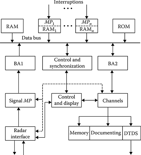
FIGURE 8.11 Microprocessor subsystem with federal structure.
The microprocessor subsystems with a completely decentralized structure, both in space and functionality, in which the local digital signal processing blocks solve the problems in the off-line mode or under the control of one block. This microprocessor subsystem allows us to increase principally the digital signal processing performance owing to the specialization of blocks carrying out the numerical calculation and best matching their structure with specific character of the realized digital signal processing algorithms. An obvious disadvantage of this microprocessor subsystem is a complexity involved in controlling this subsystem, but there are no doubts that this disadvantage can be overcome and the distributed microprocessor subsystem of digital signal processing of target return signal would be widely used in practice.

The main problems with improving the structure and elements of the considered microprocessor subsystems are as follows:

To design high-performance signal microprocessors for digital signal processing of target return signals taking into consideration solutions for both the considered and discussed problems and new problems. Obviously, one way to solve this problem is further specialization of the special-purpose microprocessors and introduction of parallel algorithms to solve the digital signal processing of target return signal problems.
To design and construct high-performance parallel (matrix, conveyer, and other types) microprocessors based on the modern and perspective element base providing the required performance for the automation of all main problems of the digital signal processing of target return signal and control process.
To design and construct the microprocessor subsystems with both uniformly and nonuni-formly distributed structure satisfying the requirements of digital signal processing hardware unification oriented to the special-purpose applications.

Considered in this section perspective avenues to develop the hardware and structure of CRS microprocessor subsystems assume the maximal parallelism in computational processes that, in the final analysis, is reduced to constructive solution of operational problems of parallel programming. Planning methods of parallel numerical calculation processes in the multimicroprocessor subsystems are related to the modern problems.

8.6 High-Performance Centralized Microprocessor Subsystem for Digital Signal Processing of Target Return Signals in Complex Radar Systems

Images

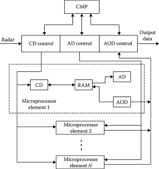
FIGURE 8.12 Microprocessor subsystem with ensemble of parallel microprocessors.

As an example of the high-performance centralized microprocessor subsystem for digital signal processing of target return signals, we consider the microprocessor subsystem with an ensemble of parallel microprocessors [23, 24]. Parallelism of independent objects during the target tracking is used by this microprocessor subsystem. Computational subsystem consists of three main constituents (see Figure 8.12): the principal microprocessor, the N independent identical microprocessors called the microprocessor elements, and the central controller of the microprocessor subsystem. The principal microprocessor is the central element of the whole microprocessor subsystem and is assigned to solve all problems that are not related to the digital signal reprocessing of target return signals. In addition, the principal microprocessor ensures all control functions of computational subsystem programs, including a translation of programs for all microprocessor elements. Independent and identical microprocessor elements, the number of which defines the microprocessor system performance, operate in parallel under the common control of the principal microprocessor. Each microprocessor element includes the following:

The arithmetical device (AD) that is used for computations made by the microprocessor element.
The associative output device (AOD) containing necessary circuits to select (to activate) the microprocessor element.
The correlation device (CD) is the high-speed data input device with addressing by content, which is designed specially for target return signal data input.
The RAM with arbitrary addressing.

The central control microprocessor coupling an ensemble of microprocessor elements with the principal microprocessor consists of three CBs that operate simultaneously. This way, a parallel digital signal processing of target return signal in AD can be matched in time with the associative data input over CD and data output over AOD. Thus, the microprocessor subsystem can realize 3N operations in parallel. The microprocessor subsystem shown in Figure 8.12 is assigned for the individual multiple targets tracking. For this purpose, the individual microprocessor element is assigned for each tracked target. During digital signal processing of the target return signals the problems of data input, linear filtering, CRS control, and data output are solved. New information about each tracked target in the form of the target pip coordinates is stored by the memory of corresponding microprocessor element using CD. Distribution of RAMs for each microprocessor element is the same. Each RAM is divided into three sections: to store new unprocessed data waiting for filtering, that is, the buffer of unprocessed data; to store the tracked target trajectory parameters obtained at the previous step of filtering; to store the requests queuing, that is, the instant of next coordinate measuring and the extrapolated target track parameters at this instant.

If we assume that clamping of new target pips to target tracks is carried out only by a single coordinate, for example, radar range, then the digital correlation signal processing algorithm is reduced to the fulfillment of the following operations:

When a new target pip comes from radar, the control block of CD interrupts arithmetical operations for all microprocessor elements and subsequently the predictable radar ranges for all tracking targets at the instant of incoming a new target pip are determined:

${\hat{R}}_{n}^{el} = {\hat{R}}_{n - 1} + R_{n - 1} (t_{n} - t_{n - 1}) . (8.50)$ ${\hat{R}}_{n}^{el} = {\hat{R}}_{n - 1} + R_{n - 1} (t_{n} - t_{n - 1}) . (8.50)$
For each predictable radar range value, the gate ΔR is determined and dimensions of the gate ΔR are loaded in comparison registers of corresponding microprocessor elements.
Parallel comparison of the radar range coordinate for new target pip with the predictable coordinates of all target tracking trajectories is carried out. If the target pip is within the limits of the gate of any tracking target, the radar range coordinate is transferred to the corresponding microprocessor element. Otherwise, we assume that a new target has been detected and we can start to accumulate information about a new target track.

Thus, in this case, a new identification time of target pips is independent of the number of tracking targets. The target track filtering is carried out by each microprocessor element using iteration of the digital signal processing algorithms. For the realization of operation of selecting the next target for queuing, the AOD is used. Checking of all tracking target by any feature is carried out by the AOD in parallel. For this reason, the time required to search the most priority target for target queuing is the same as that is required for checking a single target.

8.7 Programmable Microprocessor for Digital Signal Preprocessing of Target Return Signals in Complex Radar Systems

As an example of the high-performance CMP subsystem assigned to solve the main problems of digital signal preprocessing of target return signals we consider one possible realization version of the programmable signal microprocessor, the structure and software of which possess a definite degree of universality that allows us to interface this CMP subsystem with CRSs of different types, including radar systems of old standards during their modernization. The programmable signal microprocessor subsystem is represented in Figure 8.13 and consists of the following main elements:

The microprocessor of intraperiod digital signal processing, that is, the input microprocessor, consisting of analog-digital converter (ADC), two-channel filter to compress the linear-frequency-modulated signals in frequency domain (fast Fourier transform [FFT]), and CB. The ADC allows us to carry out a discretization in time of input signals (target return signals). The FFT microprocessor carries out FFT, convolution in frequency domain, inverse FFT, and combination of in-phase and quadrature components. The microprocessor has a structure allowing us to increase its performance.

FIGURE 8.13 Programmable signal microprocessor subsystem.
The arithmetical microprocessor consists of two parallel general-purpose microprocessors with RAM and CB. The arithmetical microprocessor allows us to realize parallel, including conveyer, computations by two identical channels and is assigned to solve all problems of interperiod digital signal processing of target return signals, namely, moving target indication, constant false alarm, target detection and resolution, target coordinate evaluation, and so on. The speed of operation of the microprocessor subsystem allows us to solve the problems of Doppler filtering. For this purpose, the FFT microprocessor is used.
The RAM as a set of RAM modules. These RAM modules can be coupled with other microprocessor subsystem elements using CB.
The interface with external objects includes 8 bidirectional I/O channels ensuring transmission of 32 digits per word. In addition, there is a wideband channel of direct memory access.
The control microprocessor assigned to solve the control problems of the microprocessor subsystem is realized as the 32-digits-per-word programmable microprocessor including RAM of larger size (capacity) and microinstruction memory.

Thus, the considered programmable microprocessor subsystem provides for the individual realization of digital signal processing using two real timescales: the intraperiod digital signal processing using the input programmable microprocessor of real time and the interperiod digital signal processing using the arithmetical microprocessor. The programmable microprocessor subsystem can be implemented in combination with a wide range of CRSs for target detection and tracking with mechanically rotating antenna. If requirements for speed of operation and memory size (capacity) cannot be satisfied by using a single-programmable-microprocessor subsystem, we can apply the programmable multimicroprocessor subsystem with controller.

8.8 Summary and Discussion

To compare the microprocessor systems between each other we can consider the following engineering data: addressness—the number of address codes used by the instruction code; number representation capacity—the control microprocessor systems are characterized by 16, 24, 32, and 64 digits per word; number representation form—there are two number representation forms: the fixed and the floating point; microprocessor speed of operation—to characterize the speed of operation of the microprocessor subsystem the statement of “rated speed” is introduced independent of the solved problem class; effective speed of operation—the average number of operations per second for the realization of the specific digital signal processing algorithm.

One of the possible ways to increase the microprocessor subsystem performance and reliability for digital signal processing in real time is to design and construct the CRS multicomputer subsystems for effectively using the digital signal processing algorithms. Computational process in the multicomputer subsystems is organized using new principles, namely, a parallel digital signal processing by several microprocessor subsystems. The main factors defining such a multicomputer subsystem structure include the end use, required performance, and memory size for the solution of given problem in totality and functional reliability taking into consideration external environment and economical factors—admissible cost and admissible energy consumption.

The homogeneous multicomputer subsystem constructed based on the principles of adjustment operation, operation of information exchange, operation of generalized conditional jump, and operation of generalized unconditional jump allows us to realize any digital signal processing algorithms. In other words, this is universal subsystem in algorithmic sense. These homogeneous multicomputer subsystems do not have any limitations in performance for the computation of complex digital signal processing algorithms and allow us to ensure the required reliability and subsystem survival under the assumption of unlimited number of elementary cells (microprocessors). The designing problem for the homogeneous multicomputer subsystems is to define the number of elementary cells ensuring the realization of the complex digital signal processing algorithms in real time and required operational reliability taking into consideration the multicomputer subsystem losses in the effective speed of operations.

The backbone multimicroprocessor subsystem combines several independent microprocessors coupled with each other in such a way that information at the output of one microprocessor comes in at the input of another microprocessor; that is, the microprocessors process information sequentially or in conveyer style. The conveyer style of digital signal processing is based on partition of the digital signal processing algorithm on a set of steps and matching in time these steps when the digital signal processing algorithm is accomplished. Advantages with the implementation of the back-bone multimicroprocessor subsystems compared to the matrix homogeneous multimicroprocessor ones are the moderate requirements with respect to inner coupling and simplicity with which the backbone multimicroprocessor subsystem’s computational power can be increased. Disadvantages are removed by organizing a priority exchange of information between the system cells.

Two types of the backbone multimicroprocessor subsystems are widely used for digital signal processing in real time: the first type, a one-dimensional inner long-distance channel operating in the time-sharing mode, and the second type, a multidimensional inner long-distance channel coupled with two-input RAM. In the backbone multimicroprocessor subsystem of the first kind all RAM and ROM, CMP, and SMP are combined by the same channel. There is a block to control the channel. This block is used in the case of conflict situations when several micro-processors address RAM simultaneously and for controlling data upload and extraction using the channel units to exchange the data. Operation of a single backbone multimicroprocessor subsystem is carried out in the following way. Each microprocessor submits, as needed, an application to the channel to address to RAM or ROM. If the channel is free then the microprocessor can access RAM or ROM immediately. Otherwise, the microprocessor is in the idle mode. The microprocessor can access RAM or ROM when the previous queries from other microprocessors are ended and there are no further high-priority queries from microprocessors. Consequently, there are high requirements to the information channel with respect to the data channel through-put. Determination of the required throughput is carried out for each specific case using methods of the queuing theory. Finally note that the said structure of the backbone multimicroprocessor subsystem has limited speed of operation defined by the data channel throughput and, in addition, with the data channel failure, the backbone multimicroprocessor subsystem stops any operation. A great advantage of the backbone multimicroprocessor subsystem is its simplicity. In the back-bone multimicroprocessor subsystem with the multidimensional inner long-distance channel, all microprocessors operate using independent asynchronous mode and all conflict situations are practically excluded. This system has very high reliability and allows us to increase the performance without any limitations. Disadvantage of the backbone multimicroprocessor subsystem with the multidimensional inner long-distance channel is the high complexity caused by the use of multiinput RAM and ROM. While designing the multimicroprocessor subsystem, the main problem is to provide the required performance by selecting the number of microprocessors to be included in the structure of this subsystem. With an increase in the number of microprocessors in the multimicroprocessor subsystem structure, a portion of overhead caused by a waiting time while microprocessor addresses RAM or ROM, simultaneously addressing common tables and operational systems, and the timetables caused by operation of the supervisory routing increase too.

The microcomputer constructed based on a microprocessor possesses high reliability and flexible universality; however, speed of operation is low. In this case, the required performance for CRS digital signal processing can be realized by organization of multiple microcomputer systems using several microprocessors. Such computer systems are called the microprocessor systems. In any microprocessor subsystem there must be an organized network providing communication between the microprocessor subsystem elements for data exchange between microcomputers. Configuration and the degree of complexity of such communications depend on the CRS digital signal processing algorithms, the distribution of operations between the microcomputers, and the acceptable number of RAM used by one microcomputer.

The QS interacts with sources of requests for queuing. In the discussed case, the targets and other interferences being in the radar coverage are considered as the sources of queuing requests. These sources interact with the QS by a request sensor—the CRS plays this role. Radar system transforms the queuing request into signals that are subjected to process. Time sequence of these signals, which is ordered during radar sensing and scanning of the controlled space, forms an input request flux for the QS. The incoming flux request service is organized by the. QS. The QS can be considered as both the device carrying out a direct request service and the device assigned to store a request queue meant for service. The QS is characterized by the following: (a) the number of devices (cells) assigned to store a request queue of the incoming signal flux (the IBA memory size); (b) the number of devices (channels) K that can serve the requests simultaneously; (c) the number of devices (cells) to accumulate and store the results of digital signal processing (the IBA memory size). The request queue is stored by IBA of microprocessor subsystem. The waiting time and the number of queued requests (the request queue length) are the random variables depending on statistical parameters of the incoming signal flux and service rate. Because the IBA size (memory capacity) is limited, the request queue length and, consequently, the waiting time of request queue are limited too. This QS is called the QS with the limited queue (the limited waiting time). Thus, the digital signal processing subsystem can be considered as the subsystem belonging to the class of QSs with limited queue.

The process of selecting a new request from a set of requests waiting queuing involves the following. After digital signal processing of immediate request, the supervisory program investigates sequentially queuing and selects for service the request possessing the greatest priority. After initiation of the corresponding routine, it is realized by the microprocessor. The queued request leaves the system, and a control is transferred to the supervisory routine again. If there are no further requests, then the supervisory routine switches on the microprocessor in the idle mode. At each instant, the microprocessor can run a single program only. For this reason, the considered. QS is called a single-channel or a single-microprocessor QS.

As a rule, we need to exercise strong limitations with respect to the waiting time for request queuing of individual signal fluxes that require assigning them by absolute priorities, for example, the requests to process the target return signals. Other requests have excess waiting time and may be assigned by relative priorities. Several requests can be served by the simple queuing procedure. Thus, we see that we need to apply mixed regulations for request queuing, investigation of which is carried out for each specific case by simulation procedures.

The required effective speed down boundary definition of the third type of control single-microprocessor subsystem operation can be considered as the initial stage of designing the microprocessor subsystem for CRS digital signal processing. The next stage involves choosing the optimal request queuing regulation. At the system design stage, we will not have sufficient information to choose the specific request queuing regulation, but we should take into consideration the following circumstances: (a) the request queuing regulation based on request queuing in turn to come in at the control single-microprocessor subsystem possesses the best performance among all the nonpriority request queuing regulations; in particular, in this case, the variance of the request queuing waiting time is minimum compared to other nonpriority request queuing regulations; (b) introduction of the priority request queuing regulation allows us to decrease essentially the request queuing waiting time for the most important requests of signal flux owing to increased delay during the queuing of signal minor fluxes; (c) in general, introduction of the priority request queuing regulations provides an equivalent performance of the control single-microprocessor subsystem compared to the request queuing one in turn. Consequently, the aforementioned values of the required minimum speed of control single-microprocessor subsystem operation provides a possibility to choose the priority request queuing regulation without any additional increase in the effective speed of operation. The minimum value of the effective speed of operation ensures the boundary values of the request queuing waiting time of the earlier-considered types of the request queuing regulations for the control single-microprocessor subsystem and related to a queue length that can be defined for the kth signal flux as l_k = λ_kt_{wait k}. Queue existence and its store are related to definite losses. To decrease these losses, the effective speed of control single-microprocessor subsystem operation must be greater than minimal one. However, in this case, the loading factor U decreases and, correspondingly, the idle time factor Q = 1 − U increases, which is not good from the point of view of hardware costs.

Requirements for RAM size and structure are defined based on the end use of the system, character and digital signal processing algorithms, and analysis of input and output signal fluxes. As a first approximation, the total RAM size (memory capacity) is defined from the formulas Q_Σ = Q_routine + Q_digit, where Q_routine is the RAM cell array assigned to store the routines of digital signal processing algorithms, control routine of computational process and operation of whole system, interruption routines, and routines controlling calculations; Q_digit is the RAM cell array assigned to store a numerical information. In turn, Q_digit can be presented in the following form: Q_digit = Q_in + Q_working + Q_out, where Q_in is the RAM cell array assigned to receive external information; Q_working is the RAM cell array participating at the calculation process; Q_out is the RAM cell array assigned to store the results of digital signal processing. In many cases, the relative independence of routine information on numerical one leads us to expediently use individual permanent memory or ROM to store the routine information. ROM uses only a reading mode. Implementation of ROM gives us a great advantage because information stored by ROM is not lost even if the power is off. In addition, ROM possesses high reliability. As for ROM size (capacity), at the initial stage of designing the digital signal processing subsystem it is possible to estimate this parameter approximately. The exact estimation is possible only after program debugging.

The problem with choosing the special-purpose microprocessors is solved based on requirements for making demands to the designed microprocessor subsystem on speed of operation, RAM and ROM sizes, and technical characteristics, reliability, overall dimensions, use, cost, and other requirements. Selection of the appropriate microprocessor depends on the degree of correspondence between a set (vector) of QoS of the selected microprocessor and a set (vector) of requirements to these quality indices. A numerical measure or criterion of effectiveness must be established to compare the selected microprocessors. However, at the initial stages of designing it is very difficult, as a rule, to establish a function between the parameters of microprocessor and generalized criterion of effectiveness as a whole. Moreover, selection of the generalized criterion, demonstrable and convenient in computational sense, is not easy. We can obtain the following results of comparison between the microprocessor parameters: (a) only one type of microprocessors from existing nomen-clature satisfies all requirements; (b) none of the microprocessors from existing nomenclature satisfies all requirements; and (c) there are several types of microprocessors from existing nomenclature satisfying all requirements. In the first case, only the microprocessor that satisfies all requirements is selected to design the microprocessor subsystem. In the second case, we need either to correct the requirements based on simplification of digital signal processing algorithms for solved problems and change an environment or to make a decision to construct a multimicroprocessor subsystem based on implementation of microprocessor of the same or different types produced by industry. In the third case, the problem with selecting the best microprocessor satisfying all requirements is solved. In this case, there are several ways to make this choice. We consider the simplest way—the ranking way.

While designing the structure of microprocessor subsystem for CRS digital signal processing of target return signals we need to consider a sequence of digital signal processing step realization and the difference in the scale of real time for each step involved in digital signal processing. An important initial condition for the synthesis of microprocessor subsystems is the selection of appropriate hardware and software that as a unit helps to solve the problems associated with CRSs. A total set of the microprocessor subsystem hardware can be divided into the following groups: (a) the micro-processor subsystem facilities providing a realization of CRS digital signal processing algorithms; (b) the communication facilities providing transmission of information from sources to users; (c) the facilities of transmission of information; and (d) the interface and commutation facilities assigned to unify the microprocessor subsystem facilities into the multimicroprocessor subsystems for the purpose of increasing the speed of operation and reliability of computations and numerical calculations. Naturally, the main microprocessor subsystem element defining its structure is a system of computing facilities. Two types of computing facilities are employed by the digital signal processing subsystems, namely, the control microprocessor subsystem and the multimicroprocessor sub-systems for specific applications providing a realization of the main digital signal processing and control algorithms, and the special-purpose high-performance microprocessors assigned mainly for target return signal filtering at the stages of the intra- and inter-period digital signal processing. The other aforementioned hardware facilities are special purpose and are assigned for SMP subsystems implemented in CRSs of special-purpose application. Questions of rational selection of hardware facilities for designing the microprocessor subsystem are essential because, in the case of special-purpose applications, dimensions and cost of such SMP subsystems outweigh the corresponding characteristics and performance of usual microprocessor systems.

Software is the programmable facility system assigned to increase the effectiveness of employing a microprocessor subsystem and decrease the work content of preliminary operation for the solution of problems by microprocessor subsystem. Software can be divided as internal and external software. In the control microprocessor, the internal software consists of the automized programming routine, operating system routine, that is, computational process control routine, and functioning control routine. The external software consists mainly of the application program library and the specific programs of CRS digital signal processing. Because the cost of designing software exceeds the cost of designing hardware, one of the main avenues of the microprocessor subsystem development is the realization of some typical software functions by hardware.

The main problems with improving the structure and elements of the considered microprocessor subsystems are the following: (a) to design the high-performance signal microprocessors for digital signal processing of target return signals, taking into consideration solutions for both considered and discussed problems and new problems (obviously, one way to solve this problem is to further specialize the special-purpose microprocessors and to introduce parallel algorithms for solving the digital signal processing of target return signal problems); (b) to design and construct high-performance parallel (matrix, conveyer, and other types) microprocessors based on modern and perspective element base providing the required performance during the automation of all main problems of CRS digital signal processing of target return signal and control process; and (c) to design and construct the microprocessor subsystems with uniformly and nonuniformly distributed structure satisfying requirements of unification of digital signal processing hardware oriented to the special-purpose applications.

References

1. Evreinov, A.V. and V.G. Choroshevskiy. 1978. Homogeneous Computer Systems. Novosibirsk, Russia: Nauka.

2. Corree, E., de Castro Dutra, I., Fiallos, M., and L.F.G. da Silva. 2010. Models for Parallel and Distributed Computation: Theory, Algorithmic Techniques and Applications. New York: Springer, Inc.

3. Dandamudi, S. 2003. Hierarchical Scheduling in Parallel and Cluster Systems. New York: Springer, Inc.

4. Milutinovic, V. 2000. Surviving the Design of Microprocessor and Multimicroprocessor Systems: Lessons Learned. New York: Wiley Interscience, Inc.

5. Shen, J.P. and M.H. Lipasti. 2004. Modern Processor Design: Fundamentals of Superscalar Processors. New York: McGraw Hill, Inc.

6. Conte, G. and D. de Corso. 1985. Multi-Microprocessor Systems for Real-Time Applications. New York: Springer, Inc.

7. Gupta, A. 1987. Multi-Microprocessors. New York: IEEE Press, Inc.

8. Parker, Y. 1984. Multi-Microprocessor Systems. San Diego, CA: Academic Press, Inc.

9. Cartsev, M.A. and V.A. Brick. 1981. Computer Systems and Synchronous Arithmetics. Moscow, Russia: Radio and Svyaz.

10. Yamanaka, N., Shiomoto, K., and E. Ok. 2005. GMPLS Technologies: Broadband Backbone Networks and Systems. Boca Raton, FL: CRC Press, Inc.

11. Kartalopoulos, S. 2010. Next Generation Intelligent Optical Networks from Access to Backbone. New York: Springer, Inc.

12. Williams, M. 2010. Broadband for Africa: Developing Backbone Communications Networks. New York: World Bank Publications, Inc.

13. Gnedenko, V.V. and I.N. Kovalenko. 1966. Queuing Theory. Moscow, Russia: Nauka.

14. Kobayqashi, H., Mark, B.L., and W. Turin. 2011. Probability, Random Processes, and Statistical Analysis: Applications to Communications, Signal Processing, Queuing Theory, and Mathematical Finance. Cambridge, U.K.: The Cambridge University Press, Inc.

15. Furmans, K. 2012. Material Handling and Production Systems Modeling—Based on Queuing Models. New York: Springer, Inc.

16. Alfa, A.S. 2010. Queuing Theory for Telecommunications. New York: Springer, Inc.

17. Tolk, A. and L.C. Jain. 2009. Complex Systems in Knowledge-Based Environments: Theory, Models, and Applications. New York: Springer, Inc.

18. Cornelius, T.L. Ed. 1996. Digital Control Systems Implementation and Computational Techniques. San Diego, CA: Academic Press, Inc.

19. Nedjah, N. 2010. Multi-Objective Swarm Intelligent Systems: Theory & Experiences. New York: Springer, Inc.

20. Yu, H.H. Ed. 2001. Programmable Digital Signal Processors: Architecture, Programming, and Applications. Boca Raton, FL: CRC Press, Inc.

21. Baese, M. 2007. Digital Signal Processing with Field Programmable Gate Arrays, 3rd Edn. New York: Springer, Inc.

22. Parhi, K.K. 1999. VLSI Digital Signal Processing Systems: Design and Implementation. New York: Wiley–Interscience Publication.

23. Kirk, D.B. and W.H. Wen-Mei. 2010. Programming Massively Parallel Processors. Burlington, MA: Morgan Kaufman Publishers.

24. McCormick, J.W., Singhoff, F., and J. Huques. 2011. Building Parallel, Embedded, and Real-Time Applications with Ada. Cambridge, U.K.: The Cambridge University Press, Inc.

..................Content has been hidden....................

You can't read the all page of ebook, please click here login for view all page.

Table of Contents for
Chapter 8 Design Principles of Digital Signal Processing Subsystems Employed by a Complex Radar System

8 Design Principles of Digital Signal Processing Subsystems Employed by a Complex Radar System

8.1 Structure and Main Engineering Dat a Of Digital Signal Processing Subsystems

8.1.1 SINGLE-COMPUTER SUBSYSTEM

8.1.2 MULTICOMPUTER SUBSYSTEM

8.1.3 MULTIMICROPROCESSOR SUBSYSTEMS FOR DIGITAL SIGNAL PROCESSING

8.1.4 MICROPROCESSOR SUBSYSTEMS FOR DIGITAL SIGNAL PROCESSI NGIN RADAR

8.2 Requirements for Effective Speed of Operation

8.2.1 MICROPROCESSOR SUBSYSTEM AS A QUEUING SYSTEM

8.2.2 FUNCTIONING ANALYSIS OF SINGLE-MICROPROCESSOR CONTROL SUBSYSTEM AS QUEUING SYSTEM

8.2.3 SPECIFICATIONS FOR EFFECTIVE SPEED OF MICROPROCESSOR SUBSYSTEM OPERATION

8.3 Requirements for Ram Size and Structure

8.4 Selection of Microprocessor for Designing the Microprocessor Subsystems

8.5 Structure and Elements of Digital Signal Processing and Complex Radar System Control Microprocessor Subsystems

8.6 High-Performance Centralized Microprocessor Subsystem for Digital Signal Processing of Target Return Signals in Complex Radar Systems

8.7 Programmable Microprocessor for Digital Signal Preprocessing of Target Return Signals in Complex Radar Systems

8.8 Summary and Discussion

References

Table of Contents for Chapter 8 Design Principles of Digital Signal Processing Subsystems Employed by a Complex Radar System

Create new playlist

Sign In

Sign Up

Table of Contents for
Chapter 8 Design Principles of Digital Signal Processing Subsystems Employed by a Complex Radar System