Chapter 14 Estimation of Probability Distribution and Density Functions of Stochastic Process

Search in book...
Toggle Font Controls
Create new playlist

Name your new playlist

Playlist description (optional)
Sign In

Email address

Password

Forgot Password?

or

Continue with Facebook

Continue with Google
Sign Up

Full Name

Email address

Confirm Email Address

Password

or

Continue with Facebook

Continue with Google

Experimental definition of the one-dimensional probability distribution function F(x) and pdf p(x) is formed in the simplest way for ergodic stochastic processes and is based on an investigation of the stochastic process within the limits of the time interval [0, T]. Actually, a researcher observes the realization x(t) of a continuous ergodic process ξ(t). An example of the realization x(t) is shown in Figure 14.1a. According to the definition of ergodic stochastic process [1], the probability distribution function F(x) can be defined approximately in the following form (see Figure 14.1a):

F * ⎛ ⎝ ⎜ ⎜ x ⎞ ⎠ ⎟ ⎟ \approx 1 T \sum ​ i = 1 N τ i, (14.1)

$F^{*} (x) \approx \frac{1}{T} {\sum^{}}_{i = 1}^{N} τ_{i}, (14.1)$

where F*(x) is the estimate of the probability distribution function F(x) defined by the total time when the value of the realization x(t) is below the level x within the limits of the observation interval [0, T].

It is natural to suppose that the larger the observation interval and the total time when the value of the realization x(t) is below the level x the closer the estimate F*(x) to the true value F(x). Thus, in the limiting case, when the observation interval [0, T] is large, the following equality

F ⎛ ⎝ ⎜ ⎜ x ⎞ ⎠ ⎟ ⎟ = P ⎡ ⎣ ⎢ ⎢ ξ ⎛ ⎝ ⎜ ⎜ t ⎞ ⎠ ⎟ ⎟ \leq x ⎤ ⎦ ⎥ ⎥ = lim T \to \infty 1 T \sum ​ i = 1 N τ i (14.2)

$F (x) = P [ξ (t) \leq x] = \lim_{T \to \infty} \frac{1}{T} {\sum^{}}_{i = 1}^{N} τ_{i} (14.2)$

is satisfied.

The approximation accuracy of the defined experiment estimate F*(x) to the true probability distribution function F(x) is characterized by the random variable

Δ F (x) = F (x) - F * (x) . (14.3)

$Δ F (x) = F (x) - F^{*} (x) . (14.3)$

Based on (14.3), we obtain the bias of the probability distribution function estimate

b [F * (x)] = ⟨ Δ F (x) ⟩ = F (x) - ⟨ F * (x) ⟩ (14.4)

$b [F^{*} (x)] = 〈 Δ F (x) 〉 = F (x) - 〈 F^{*} (x) 〉 (14.4)$

and the variance of the probability distribution function estimate

Var {F * (x)} = ⟨ [F * (x) - ⟨ F * (x) ⟩] 2 ⟩, (14.5)

$Var {F^{*} (x)} = 〈 {[F^{*} (x) - 〈 F^{*} (x) 〉]}^{2} 〉, (14.5)$

Images

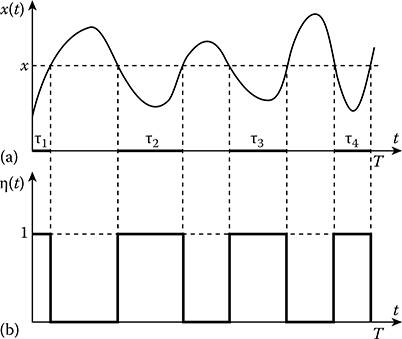
FIGURE 14.1 (a) Realization of stochastic process within the limits of the observation interval [0, T]; (b) Sequence of rectangular pulses formed in accordance with the nonlinear inertialess transformation (14.13).

which are the functions both of the averaging time and of the reference level.

The one-dimensional pdf of ergodic stochastic process is defined based on the following relationship:

p ⎛ ⎝ ⎜ ⎜ x ⎞ ⎠ ⎟ ⎟ = d F ( x ) d x = lim T \to \infty 1 T Δ x \sum ​ N i = 1 τ i' . (14.6)

$p (x) = \frac{d F (x)}{d x} = \lim_{T \to \infty} \frac{1}{T Δ x} {\sum^{}}_{N}^{i = 1} τ_{i}' . (14.6)$

As we can see, (14.6) is the ratio between the probabilities of event that the values of stochastic process ξ(t) are within the limits of the interval [x − 0.5dx; x + 0.5dx] and dx, where dx is the interval length. In other words,

p [x (t)] = P { ( x - 0.5 d x ) \leq x ( t ) \leq ( x + 0.5 d x ) } d x . (14.7)

$p [x (t)] = \frac{P {(x - 0.5 d x) \leq x (t) \leq (x + 0.5 d x)}}{d x} . (14.7)$

As we can see from (14.6), ∑Ni=1τi' $\sum_{i = 1}^{N} τ_{i}'$ is the total time when the values of the realization x(t) of stochastic process are within the limits of the interval [x ± 0.5dx] (see Figure 14.2a).

Images

FIGURE 14.2 (a) Realization of stochastic process within the limits of the observation interval [0, T] with quantization by amplitude within the limits of the interval [x ± 0.5⋄x]; (b) Sequence of rectangular pulses formed in accordance with the nonlinear transformation (14.23).

In practice, a measurement of the pdf is carried out within the limits of the fixed time interval [0, T]. The interval Δx takes the finite value and Δx ≠ 0. In this case, the pdf defined by experiment can be presented in the following form:

p * (x) = 1 T Δ x \sum i = 1 N τ i' (14.8)

$p^{*} (x) = \frac{1}{T Δ x} \sum_{i = 1}^{N} τ_{i}' (14.8)$

and is different from the true values of the pdf p(x) on the random variable defined as

Δ p (x) = p (x) - p * (x) . (14.9)

$Δ p (x) = p (x) - p^{*} (x) . (14.9)$

The bias and variance of the pdf estimate can be presented in the following forms:

b [p * (x)] = p (x) - ⟨ p * (x) ⟩, (14.10)

$b [p^{*} (x)] = p (x) - 〈 p^{*} (x) 〉, (14.10)$

Var {p * (x)} = ⟨ [p * (x) - ⟨ p * (x) ⟩] 2 ⟩ . (14.11)

$Var {p^{*} (x)} = 〈 {[p^{*} (x) - 〈 p^{*} (x) 〉]}^{2} 〉 . (14.11)$

According to (14.8), the pdf is defined experimentally like the average value of the pdf within the limits of the interval [x ± 0.5dx]. Because of this, from the viewpoint of approximation of the measured pdf to its true value at the level x, it is desirable to decrease the interval Δx. However, a decrease in the Δx at the fixed observation time interval [0, T] leads to a decrease in time of the stochastic process within the limits of the interval Δx and, consequently, to an increase in the variance of the pdf estimate owing to a decrease in the statistical data sample based on which the decision about the pdf p(x) magnitude is made. Therefore, there is an optimal value of the interval Δx, under which the dispersion of the pdf estimate

D ˆ [p * (x)] = b 2 [p * (x)] + Var {p * (x)} (14.12)

$\hat{D} [p^{*} (x)] = b^{2} [p^{*} (x)] + Var {p^{*} (x)} (14.12)$

takes the minimal magnitude at the fixed observation time T.

There are several ways to measure the total time of stochastic process observation below the given level or within its limits. Consider these ways applied to an experimental definition of the probability distribution function estimate F*(x). The first way is the direct measurement of total time when a magnitude of the realization x(t) of continuous ergodic process ξ(t) is below the fixed level x. In this case, the realization x(t) is transformed into the sequence of rectangular pulses η(t) (see the Figure 14.1b) with the unit amplitude and duration τ_i equal to the time when a magnitude of the realization x(t) of continuous ergodic process ξ(t) is below the fixed level x. This transformation takes the following form:

η (t) = {10 at at x (t) \leq x, x (t) > x . (14.13)

$η (t) = {\begin{array}{l} 1 & at & x (t) \leq x, \\ 0 & at & x (t) > x . \end{array} (14.13)$

Then, the area occupied by all rectangular pulses is equal by value to the total time when the realization x(t) of continuous ergodic process ξ(t) is below the fixed level x:

\sum ​ i = 1 N τ j = \int ​ 0 T η ⎛ ⎝ ⎜ ⎜ ⎜ ⎜ t ⎞ ⎠ ⎟ ⎟ ⎟ ⎟ d t . (14.14)

${\sum^{}}_{i = 1}^{N} τ_{j} = {\int^{}}_{0}^{T} η (t) d t . (14.14)$

As a result, the probability distribution function estimate takes the following form:

F * ⎛ ⎝ ⎜ ⎜ ⎜ ⎜ t ⎞ ⎠ ⎟ ⎟ ⎟ ⎟ = 1 T \int ​ 0 T η ⎛ ⎝ ⎜ ⎜ ⎜ ⎜ t ⎞ ⎠ ⎟ ⎟ ⎟ ⎟ d t . (14.15)

$F^{*} (t) = \frac{1}{T} {\int^{}}_{0}^{T} η (t) d t . (14.15)$

The nonlinear inertialess transformation (14.13) is carried out without any problems by corresponding limitations in amplitudes and threshold devices.

The second way to define and measure the probability distribution function is based on computation of the number of quantized by amplitude and duration of the sampled pulses. In this case, at first, the continuous realization x(t) of stochastic process ξ(t) is transformed by the corresponding pulse modulator into sampled sequence x_i and comes in at the input of the threshold device with the threshold level x. Then, a ratio of the number of pulses N_x that do not exceed the threshold to the total number of pulses N corresponding to the observation time interval [0, T] is equal by value to the probability distribution function estimate, i.e.,

F * (x) = N x N . (14.16)

$F^{*} (x) = \frac{N_{x}}{N} . (14.16)$

The total number of pulses is associated with the observation time accurate within a single pulse by the following relationship:

N = T T p, (14.17)

$N = \frac{T}{T_{p}}, (14.17)$

where T_p is the period of pulse repetition.

The number of pulses N_x that do not exceed the threshold x can be presented in the form of summation of the pulses with unit amplitude

N x = \sum ​ i = 1 N η i, (14.18)

$N_{x} = {\sum^{}}_{i = 1}^{N} η_{i}, (14.18)$

where

η i = {10 at at x i \leq x, x i > x . (14.19)

$η_{i} = {\begin{array}{l} 1 & at & x_{i} \leq x, \\ 0 & at & x_{i} > x . \end{array} (14.19)$

Then the probability distribution function estimate takes the following form:

F * ⎛ ⎝ ⎜ ⎜ x ⎞ ⎠ ⎟ ⎟ = 1 N \sum ​ i = 1 N η i . (14.20)

$F^{*} (x) = \frac{1}{N} {\sum^{}}_{i = 1}^{N} η_{i} . (14.20)$

The number of pulses N and N_x is defined by various analog and digital counters. The digital counters are preferable. In practice, it is convenient to employ the nonlinear transformations of the following form:

η 1 (t) = 1 - η (t) = {10 at at x (t) \geq x, x (t) < x . (14.21)

$η_{1} (t) = 1 - η (t) = {\begin{array}{l} 1 & at & x (t) \geq x, \\ 0 & at & x (t) < x . \end{array} (14.21)$

In this case, we use the following probability distribution function:

F 1 (x) = 1 - F (x) . (14.22)

$F_{1} (x) = 1 - F (x) . (14.22)$

This statement is correct with respect to the discrete stochastic process. Experimental definition of the pdf of ergodic stochastic process is carried out in an analogous way. In the case of the first method, we carry out the following nonlinear transformation (see Figure 14.2b):

χ (t) = {10 at at x - 0.5 Δ x \leq x (t) \leq x + 0.5 Δ x, x (t) > x (t) < x - 0.5 Δ x, x + 0.5 Δ x . (14.23)

$χ (t) = {\begin{array}{l} 1 & at & x - 0.5 Δ x \leq x (t) \leq x + 0.5 Δ x, \\ 0 & at & x (t) > x (t) < x - 0.5 Δ x, x + 0.5 Δ x . \end{array} (14.23)$

In the case of the second method, using a computation of pulses, we carry out the following nonlinear transformation:

χ j = {10 at at x - 0.5 Δ x \leq x i \leq x + 0.5 Δ x, x i < x - 0.5 Δ x, x i > x + 0.5 Δ x . (14.24)

$χ_{j} = {\begin{array}{l} 1 & at & x - 0.5 Δ x \leq x_{i} \leq x + 0.5 Δ x, \\ 0 & at & x_{i} < x - 0.5 Δ x, x_{i} > x + 0.5 Δ x . \end{array} (14.24)$

Then, an experimental measurement of the stochastic process pdf is reduced to the following procedures:

p * ⎛ ⎝ ⎜ x ⎞ ⎠ ⎟ = 1 T Δ x \int 0 T χ ⎛ ⎝ ⎜ t ⎞ ⎠ ⎟ d t (14.25)

$p^{*} (x) = \frac{1}{T Δ x} \int_{0}^{T} χ (t) d t (14.25)$

and

p * ⎛ ⎝ ⎜ ⎜ x ⎞ ⎠ ⎟ ⎟ = 1 N Δ x \sum ​ i = 1 N χ i . (14.26)

$p^{*} (x) = \frac{1}{N Δ x} {\sum^{}}_{i = 1}^{N} χ_{i} . (14.26)$

14.2 Characteristics of Probability Distribution Function Estimate

Determine the bias and variance of the probability distribution function estimate based on the direct measurement of the total time when the realization x(t) of continuous ergodic process ξ(t) is below the fixed level x according to (14.15). Deviation of measured value of the probability distribution function estimate F*(x) with respect to the true value F(x) can be presented as follows:

Δ F ⎛ ⎝ ⎜ ⎜ ⎜ ⎜ x ⎞ ⎠ ⎟ ⎟ ⎟ ⎟ = 1 T \int ​ 0 T η ⎛ ⎝ ⎜ ⎜ ⎜ ⎜ t ⎞ ⎠ ⎟ ⎟ ⎟ ⎟ d t - F (x) . (14.27)

$Δ F (x) = \frac{1}{T} {\int^{}}_{0}^{T} η (t) d t - F (x) . (14.27)$

According to (14.13), the mathematical expectation of realizations η(t) can be presented in the following form:

⟨ η (t) ⟩ = P ⎡ ⎣ ⎢ ξ ⎛ ⎝ ⎜ r ⎞ ⎠ ⎟ \leq x ⎤ ⎦ ⎥ = \int - \infty x p (x') d x' = F (x) . (14.28)

$〈 η (t) 〉 = P [ξ (r) \leq x] = \int_{- \infty}^{x} p (x') d x' = F (x) . (14.28)$

As we can see from (14.27), the probability distribution function estimate is unbiased. In (14.28), p(x′) is the one-dimensional pdf of the investigated stochastic process.

Define the correlation function of the probability distribution function estimate F*(x) at various levels x₁ and x₂:

⟨ Δ F (x 1) Δ F (x 2) ⟩ = R F ⎛ ⎝ ⎜ ⎜ ⎜ ⎜ x 1, x 2 ⎞ ⎠ ⎟ ⎟ ⎟ ⎟ = 1 T 2 \int ​ 0 T \int ​ 0 T ⟨ η (t 1) η (t 2) ⟩ d t 1 d t 2 - F ⎛ ⎝ ⎜ ⎜ ⎜ ⎜ x 1 ⎞ ⎠ ⎟ ⎟ ⎟ ⎟ F ⎛ ⎝ ⎜ ⎜ ⎜ ⎜ x 2 ⎞ ⎠ ⎟ ⎟ ⎟ ⎟ . (14.29)

$〈 Δ F (x_{1}) Δ F (x_{2}) 〉 = R_{F} (x_{1}, x_{2}) = \frac{1}{T^{2}} {\int^{}}_{0}^{T} {\int^{}}_{0}^{T} 〈 η (t_{1}) η (t_{2}) 〉 d t_{1} d t_{2} - F (x_{1}) F (x_{2}) . (14.29)$

The instantaneous function 〈η(t₁)η(t₂)〉 of the stochastic process obtained as a result of nonlinear operation given by (14.13) is numerically equal to the probability of joint event that ξ(t₁) ≤ x₁ and ξ(t₂) ≤ x₂, i.e., a value of the two-dimensional probability distribution function F(x₁, x₂; τ) at the points x₁ and x₂:

F ⎛ ⎝ ⎜ x 1, x 2; τ ⎞ ⎠ ⎟ = ⟨ η (t 1) η (t 2) ⟩ = P ⎡ ⎣ ⎢ ξ ⎛ ⎝ ⎜ r 1 ⎞ ⎠ ⎟ \leq x 1, ξ ⎛ ⎝ ⎜ t 2 ⎞ ⎠ ⎟ \leq x 2 ⎤ ⎦ ⎥ = \int - \infty x 1 \int - \infty x 1 p 2 (x' 1, x' 2; τ) d x' 1 d x' 2, (14.30)

$F (x_{1}, x_{2}; τ) = 〈 η (t_{1}) η (t_{2}) 〉 = P [ξ (r_{1}) \leq x_{1}, ξ (t_{2}) \leq x_{2}] = \int_{- \infty}^{x_{1}} \int_{- \infty}^{x_{1}} p_{2} (x_{1}^{'}, x_{2}^{'}; τ) d x_{1}^{'} d x_{2}^{'}, (14.30)$

where p2(x′1,x′2;τ) $p_{2} (x_{1}^{'}, x_{2}^{'}; τ)$ is the two-dimensional pdf of the investigated stochastic process. In the case of a stationary stochastic process, the two-dimensional pdf depends only on the absolute difference in time instants τ = t₂ − t₁. For this reason, the instantaneous function given by (14.30) also depends only on the absolute difference in time instants τ = t₂ − t₁. Based on this fact, the double integral in (14.29) can be transformed into a single integral. For this purpose, introduce new variables τ = t₂ − t₁ and t₁ = t and change the order of integration taking into consideration a parity of the two-dimensional probability distribution function F(x₁, x₂; τ) = F(x₁, x₂; −τ). As a result, we obtain

\int ​ 0 T \int ​ 0 T ⟨ η (t 1) η (t 2) ⟩ d t 1 d t 2 = 2 T \int ​ 0 T (1 - τ T) F ⎛ ⎝ ⎜ ⎜ ⎜ ⎜ x 1, x 2; τ ⎞ ⎠ ⎟ ⎟ ⎟ ⎟ d τ . (14.31)

${\int^{}}_{0}^{T} {\int^{}}_{0}^{T} 〈 η (t_{1}) η (t_{2}) 〉 d t_{1} d t_{2} = 2 T {\int^{}}_{0}^{T} (1 - \frac{τ}{T}) F (x_{1}, x_{2}; τ) d τ . (14.31)$

Substituting (14.31) into (14.29), we obtain

R F ⎛ ⎝ ⎜ ⎜ ⎜ ⎜ x 1, x 2 ⎞ ⎠ ⎟ ⎟ ⎟ ⎟ = 2 T \int ​ 0 T (1 - τ T) F ⎛ ⎝ ⎜ ⎜ ⎜ ⎜ x 1, x 2; τ ⎞ ⎠ ⎟ ⎟ ⎟ ⎟ d τ - F ⎛ ⎝ ⎜ ⎜ ⎜ ⎜ x 1 ⎞ ⎠ ⎟ ⎟ ⎟ ⎟ F ⎛ ⎝ ⎜ ⎜ ⎜ ⎜ x 2 ⎞ ⎠ ⎟ ⎟ ⎟ ⎟ . (14.32)

$R_{F} (x_{1}, x_{2}) = \frac{2}{T} {\int^{}}_{0}^{T} (1 - \frac{τ}{T}) F (x_{1}, x_{2}; τ) d τ - F (x_{1}) F (x_{2}) . (14.32)$

The variance of the probability distribution function estimate at the level x is defined by (14.32) substituting x₁ = x₂ = x:

$Var {F^{*} (x)} = \frac{2}{T} {\int^{}}_{0}^{T} (1 - \frac{τ}{T}) F (x, x; τ) d τ - F^{2} (x) . (14.33)$

By analogous method, we can define characteristics under discrete transformation of the stochastic process. In this case, the deviation of the probability distribution function estimate with respect to its true value can be presented in the following form:

$Δ F (x) = \frac{1}{N} {\sum^{}}_{i = 1}^{N} η_{i} - F (x) . (14.34)$

As we can see, the probability distribution function estimate is unbiased and the correlation function of the probability distribution function estimate at different levels x₁ and x₂ can be written in the following form:

$R_{F} (x_{1}, x_{2}) = \frac{1}{N^{2}} {\sum^{}}_{i = 1, j = 1}^{N} 〈 η_{i} η_{j} 〉 - F (x_{1}) F (x_{2}), (14.35)$

where

$〈 η_{i} η_{j} 〉 = F [x_{1}, x_{2}; (i - j) T_{p}] = \int_{- \infty}^{x_{1}} \int_{- \infty}^{x_{1}} p_{2} [x_{1}^{'}, x_{2}^{'}; (i - j) T_{p}] d x_{1}^{'} d x_{2}^{'} . (14.36)$

The double sum in (14.35) can be presented in the following form:

${\sum^{}}_{i = 1, j = 1}^{N} 〈 η_{i} η_{j} 〉 = N 〈 η_{j}^{2} 〉 + {\sum^{}}_{i = 1, j = 1 i \neq j}^{N} 〈 η_{i} η_{j} 〉 . (14.37)$

The first term in (14.37) depends on the relationship between values x₁ and x₂ and can be presented in the following form:

$N 〈 η_{j}^{2} 〉 = {\begin{array}{l} N F (x_{1}) & if x_{1} \leq x_{2}, \\ N F (x_{2}) & if x_{2} \leq x_{1} . \end{array} (14.38)$

Actually, at x₁ < x₂, the probability of joint event that ξ ≤ x₁ and ξ ≤ x₂ is not equal to zero if and only if ξ ≤ x₁. In this case, the inequality ξ ≤ x₂ is satisfied with the probability equal to unit. Therefore, the probability of the joint event is equal to the probability that ξ ≤ x₁. For the second term in (14.37), we can introduce a new summation index k = i − j and change the order of summation. As a result, we obtain

${\sum^{}}_{i = 1, j = 1 i \neq j}^{N} F [x_{1}, x_{2}; (i - j) T_{p}] = 2 {\sum^{}}_{k = 1}^{N - 1} (N - k) F [x_{1}, x_{2}; k T_{p}] . (14.39)$

Substituting (14.38) and (14.39) into (14.35), the correlation function of the probability distribution function estimate F*(x) takes the following form:

$R_{F} (x_{1}, x_{2}) = {\begin{array}{l} \frac{F (x_{1})}{N} + \frac{2}{N} \sum_{k = 1}^{N - 1} (1 - \frac{k}{N}) F [x_{1}, x_{2}; k T_{p}] - F (x_{1}) F (x_{2}), & x_{1} \leq x_{2}, \\ \frac{F (x_{2})}{N} + \frac{2}{N} {\sum^{}}_{k = 1}^{N - 1} (1 - \frac{k}{N}) F [x_{1}, x_{2}; k T_{p}] - F (x_{1}) F (x_{2}), & x_{1} \geq x_{2} . \end{array} (14.40)$

The variance of the correlation function of the probability distribution function estimate F*(x) of the stochastic process is defined based on (14.40) by substituting x₁ = x₂ = x:

$Var {F^{*} (x)} = \frac{F (x)}{N} + \frac{2}{N} {\sum^{}}_{k = 1}^{N - 1} (1 - \frac{k}{N}) F [x, x; k T_{p}] - F^{2} (x) . (14.41)$

If samples are uncorrelated, then the correlation function given by (14.40) is simplified since at k ≠ 0

$F [x_{1}, x_{2}; k T_{p}] = F (x_{1}) F (x_{2}) . (14.42)$

As a result, we obtain

$R_{F} (x_{1}, x_{2}) = {\begin{array}{l} \frac{F (x_{1}) [1 - F (x_{2})]}{N}, & x_{1} \leq x_{2}, \\ \frac{F (x_{2}) [1 - F (x_{1})]}{N}, & x_{1} \geq x_{2} . \end{array} (14.43)$

In doing so, the variance of the probability distribution function estimate F*(x) of the stochastic process takes the following form:

$Var {F^{*} (x)} = \frac{F (x) [1 - F (x)]}{N} . (14.44)$

As we can see from (14.44), the variance of the probability distribution function estimate F*(x) of the stochastic process depends essentially on the level x and reaches the maximum

${Var}_{\max} {F^{*} (x)} = \frac{1}{4 N} (14.45)$

at the level x corresponding to the condition F(x) = 0.5.

In addition to the finite observation time period of the realization x(t) of continuous ergodic process ξ(t), the characteristics of the probability distribution function estimate F*(x) of the stochastic process depends also on the stability of the threshold level that can possess a random component characterized by the value δ, i.e., instead of the level x we use the level x + δ in practice. Then, the obtained characteristics of the probability distribution function estimate F*(x) of stochastic process are conditional, and to obtain the unconditional characteristics of the probability distribution function estimate F*(x) of stochastic process, there is a need to employ an averaging by all possible values of the random variable δ. We assume that the correlation interval of the random variable δ is much more in comparison with the observation time interval [0, T]. Consequently, we can think that the random variable δ does not change during measurement time of the probability distribution function estimate F*(x) of stochastic process and has the same statistical characteristics for all possible values x. Additionally, it is natural to suppose that random variations of the threshold are negligible and a difference between F(x + δ) and F(x) is very small in average sense. In this case, the probability distribution function F(x + δ) can be expanded in Taylor series about a point x and can be limited by the first three terms of expansion:

$F (x + δ) \approx F (x) + δ p (x) + 0.5 δ^{2} \frac{d p (x)}{d x} . (14.46)$

Averaging (14.46) by realizations of the random variable δ, we obtain

$〈 F (x + δ) 〉 \approx F (x) + E_{δ} p (x) + 0.5 D_{δ} \frac{d p (x)}{d x}, (14.47)$

where E_δ and D_δ are the mathematical expectation and dispersion of random variations of the threshold value x. Based on (14.27) and (14.34), we obtain that the random variations of the threshold level lead to the bias of the probability distribution function estimate F*(x) of stochastic process:

$b [F^{*} (x)] = E_{δ} p (x) + 0.5 D_{δ} \frac{d p (x)}{d x} . (14.48)$

Naturally, the presence of random variable δ leads to an increase in the variance of the probability distribution function estimate F*(x) of stochastic process.

14.3 Variance of Probability Distribution Function Estimate

14.3.1 GAUSSIAN STOCHASTIC PROCESS

The two-dimensional pdf of a Gaussian stochastic process with zero mathematical expectation is defined in the following form:

$p_{2} (x_{1}, x_{2}; τ) = \frac{1}{2 π σ^{2} \sqrt{1 - ℛ^{2} (τ)}} \exp {- \frac{x_{1}^{2} - 2 ℛ (τ) x_{1} x_{2} + x_{2}^{2}}{2 σ^{2} [1 - ℛ^{2} (τ)]}}, (14.49)$

where

σ² is the variance
ℛ(τ) is the normalized correlation function of the investigated stochastic process

However, the written form of the two-dimensional pdf of Gaussian stochastic process with zero mathematical expectation in (14.49) does not allow us to obtain the formulas for the variance of the probability distribution function estimate F*(x) that are convenient for further analysis. Therefore, we present the two-dimensional pdf of Gaussian stochastic process with zero mathematical expectation in the form of a series with respect to derivatives from the Gaussian Q-function, i.e., Q(x) given by (12.157), where we assume that the mathematical expectation is equal to zero (E = 0):

$p_{2} (x_{1}, x_{2}; τ) = \frac{1}{σ^{2}} {\sum^{}}_{v = 0}^{\infty} {1 - Q^{v + 1} (\frac{x_{1}}{o})} {1 - Q^{v + 1} (\frac{x_{2}}{o})} \frac{ℛ^{v} (τ)}{v!} . (14.50)$

Substituting (14.50) into (14.30), we obtain

$F (x_{1}, x_{2}; τ) = {1 - Q^{v + 1} (\frac{x_{1}}{σ})} {1 - Q^{v + 1} (\frac{x_{2}}{σ})} + {\sum^{}}_{v = 0}^{\infty} {1 - Q^{v + 1} (\frac{x_{1}}{σ})} {1 - Q^{v + 1} (\frac{x_{2}}{σ})} \frac{ℛ^{v} (τ)}{v!} . (14.51)$

Taking into consideration that in the case of Gaussian stochastic process

$F (x) = 1 - Q (\frac{x}{σ}), (14.52)$

the correlation function given by (14.32) and the variance given by (14.33) of the probability distribution function estimate F*(x) take the following form:

$R_{F} (x_{1}, x_{2}) = {\sum^{}}_{v = 0}^{\infty} \frac{1}{v!} {1 - Q^{v} (\frac{x_{1}}{σ})} {1 - Q^{v} (\frac{x_{2}}{σ})} \frac{2}{T} {\int^{}}_{0}^{T} (1 - \frac{τ}{T}) ℛ^{v} (τ) d τ; (14.53)$

$Var {F^{*} (x)} = {\sum^{}}_{v = 0}^{\infty} \frac{1}{v!} {1 - Q^{v} (\frac{x_{1}}{σ})}^{2} \frac{2}{T} {\int^{}}_{0}^{T} (1 - \frac{τ}{T}) ℛ^{v} (τ) d τ . (14.54)$

Since

$\begin{matrix} | Q^{v} (- z) | = | Q^{v} (z) |, & v = 1, 2, ..., \end{matrix} (14.55)$

based on (14.54), we obtain that the variance Var{F*(x)} of the probability distribution function estimate F*(x) is the even function with respect to the threshold level x.

Table 14.1 represents the values of coefficients

$a_{v} = \frac{1}{v!} [1 - Q^{v} (z)]^{2} (14.56)$

as a function of the normalized level

$z = \frac{x}{σ} . (14.57)$

TABLE 14.1
Values of the Coefficients a_v = (1/v!)[1 − Q^v(z)]² as a Function of the Normalized Level z = x/σ

Images

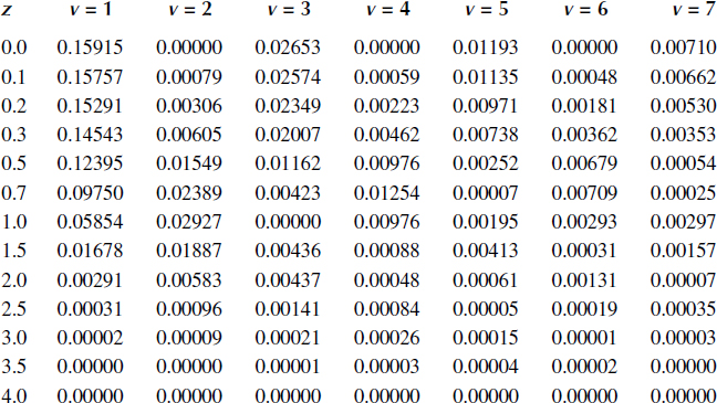
As we can see from Table 14.1, the a_v defining the variance of the probability distribution function estimate F*(x) of Gaussian stochastic process decreases with an increase in the number v. Taking into consideration that in the case of stochastic processes the factor

$c_{v} = \frac{2}{T} {\int^{}}_{0}^{T} (1 - \frac{τ}{T}) ℛ^{v} (τ) d τ (14.58)$

decreases also with an increase in the number v, in practice, we can be limited by the first 5-7 terms of series expansion.

When the observation time interval [0, T] is much more than the correlation interval of stochastic process, as earlier, the coefficients c_v can be approximated by

$c_{v} \approx \frac{2}{T} {\int^{}}_{T}^{T} ℛ^{v} (τ) d τ . (14.59)$

If, in addition to the condition T ≫ τ_cor we assume that T → ∞, then, according to (14.59) and (14.54) the variance of the probability distribution function estimate F*(x) of the Gaussian stochastic process tends to approach zero, which should be expected; i.e., the probability distribution function estimate F*(x) of the Gaussian stochastic process is consistent.

In the case when the observation time is lesser than the correlation interval of the stochastic process, i.e., T < τ_cor, we have

$Var {F^{*} (x)} \approx {\sum^{}}_{v = 1}^{\infty} a_{v} . (14.60)$

Formula (14.60) characterizes the maximal variance of the probability distribution function estimate F*(x) of Gaussian stochastic process.

As an example, consider the Gaussian stochastic process with the exponential normalized correlation function given by (12.13). Substituting (12.13) into (14.58), we obtain

$c_{v} = \frac{2}{p^{2} v^{2}} [\exp (- p v) + p v - 1], (14.61)$

where p is given by (12.140). In doing so, if p ≫ 1, then

$c_{v} \approx \frac{2}{p v} . (14.62)$

The root-mean-square deviation σ{F*(x)} of measurements of the probability distribution function of Gaussian stochastic process as a function of the normalized level z for various values of p is presented in Figure 14.3. As we can see from Figure 14.3, the maximal values of σ{F*(x)} are obtained at the zero level.

The maximal value of σ{F*(x)} as a function of the parameter p given by (12.40) is shown in Figure 14.4. As we can see from Figure 14.4 and based on (14.54) and (14.61), the variance of the probability distribution function estimate F*(x) decreases linearly as a function of p starting from p ≥ 10. This graph allows us to define the minimal required time to observe a realization of the Gaussian stochastic process when the maximal value of variance is not more than the previously given definite magnitude. For example, if we require that σ{F*(x)} ≤ 0.01, the condition p ≥ 3000 should be satisfied.

Images

FIGURE 14.3 Root-mean-square deviations σ{F*(x)} as a function of the normalized level z. Gaussian stochastic process.

Images

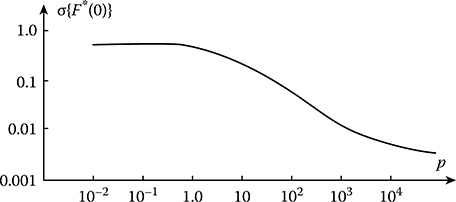
FIGURE 14.4 Maximal value of σ{F*(0)} as a function of p. Gaussian stochastic process.

When we investigate a discrete Gaussian stochastic process, the variance of the probability distribution function estimate F*(x) is defined as

$Var {F^{*} (x)} = \frac{1}{N} {1 - Q (\frac{x}{σ})} Q (\frac{x}{σ}) + {\sum^{}}_{v = 1}^{\infty} \frac{1}{v!} {1 - Q^{v} (\frac{x}{σ})}^{2} c_{v}^{'}, (14.63)$

where

$c_{v}^{'} = \frac{2}{N} {\sum^{}}^{}_{k = 1}^{N - 1} (1 - \frac{k}{N}) ℛ^{v} (k T_{p}) . (14.64)$

As applied to the exponential normalized correlation function

$ℛ^{v} (k T_{p}) = \exp {- α | k T_{p} |}, (14.65)$

(14.64) can be presented in the following form [2]:

$c_{v}^{'} = \frac{2}{N} \times \frac{\exp {- v α T_{p}} {1 - \exp {- v α T_{p}} + N^{- 1} {\exp {- v α T_{p}} - 1}}}{{1 - \exp {- v α T_{p}}}^{2}} . (14.66)$

TABLE 14.2
Normalized Correlation Function (14.68) as a Function of the Normalized Threshold Level z

Images

At N ≫ 1

$c_{v}^{'} \approx \frac{2}{N} \times \frac{\exp {- v α T_{p}}}{1 - \exp {- v α T_{p}}} . (14.67)$

In the case of uncorrelated samples, we have $c_{v}^{'} = 0$ . As a result, (14.63) coincides with (14.44).

Thus, (14.63) demonstrates that the variance of the probability distribution function estimate F*(x) of stochastic process by correlated samples increases in comparison with the variance of the probability distribution function estimate F*(x) of stochastic process by uncorrelated samples of the same sample size N.

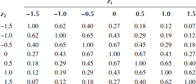
Table 14.2 represents the normalized correlation function

$ρ (x_{1}, x_{2}) = \frac{R_{F} (x_{1}, x_{2})}{\sqrt{Var {F^{*} (x_{1})} Var {F^{*} (x_{2})}}} (14.68)$

of the probability distribution function estimate F*(x) of stochastic process for various values of the threshold level z computed based on (14.43) in the case of uncorrelated samples. As we can see from Table 14.2, there is a high correlation between the probability distribution function estimations F*(x) of stochastic process.

14.3.2 RAYLEIGH STOCHASTIC PROCESS

Two-dimensional pdf of Rayleigh stochastic process ξ(t) can be presented in the following form [1]:

$p_{2} (x_{1}, x_{2}; τ) = \frac{x_{1} x_{2}}{σ^{4} [1 - ℛ^{2} (τ)]} \exp {- \frac{x_{1}^{2} + x_{2}^{2}}{2 σ^{2} [1 - ℛ^{2} (τ)]}} I_{0} {\frac{x_{1} x_{2}}{σ^{2}} \times \frac{ℛ (τ)}{1 - ℛ^{2} (τ)}}, (14.69)$

where

I₀(z) is the zero-order Bessel function of imaginary argument
σ² and ℛ(τ) are the parameters of the pdf associated with the initial second moment ξ(t) and the normalized correlation function ρ(τ) of Rayleigh stochastic process by (12.165)

Introduce new variables

$\begin{matrix} y_{1} = \frac{x_{1}^{2}}{2 σ^{2}} & and & y_{2} = \frac{x_{2}^{2}}{2 σ^{2}} \end{matrix} . (14.70)$

New top integration limits in (14.30) correspond to z₁ = y₁ and z₂ = y₂. New two-dimensional pdf can be presented by expansion in series using the orthogonal Laguerre polynomials [2]:

$p_{2} (x_{1}, x_{2}; τ) = \exp (- y_{1} - y_{2}) {\sum^{}}_{v = 0}^{\infty} \frac{L_{v} (y_{1}) L_{v} (y_{2}) ℛ^{2 v} (τ)}{{(v!)}^{2}}, (14.71)$

where L_v(y) is the Laguerre polynomial satisfying the following definition:

$L_{v} (y) = \exp {y} \frac{d^{v} [y \exp (- y)]}{d y^{v}} = {\sum^{}}_{μ = 0}^{v} {(- 1)}^{μ} C_{v}^{μ} \frac{v!}{μ!} y^{μ}, (14.72)$

where

$C_{v}^{μ} = \frac{v!}{μ! (v - μ)!}; (14.73)$

$L_{0} (y) = 1; (14.74)$

$L_{1} (y) = - y + 1. (14.75)$

Substituting (14.71) into (14.30), we obtain

$F (x_{1}, x_{2}; τ) = [1 - \exp (- z_{1})] [1 - \exp (- z_{2})] + {\sum^{}}_{v = 1}^{\infty} \frac{ℛ^{2 v} (τ)}{{(v!)}^{2}} {\int^{}}_{0}^{z_{1}} \exp (- y_{1}) L_{v} (y_{1}) d y_{1} {\int^{}}_{0}^{z_{2}} \exp (- y_{2}) L_{v} (y_{2}) d y_{2}, (14.76)$

where

${\begin{array}{l} z_{1} = \frac{x_{1}^{2}}{2 σ^{2}}; \\ z_{2} = \frac{x_{2}^{2}}{2 σ^{2}} . \end{array} (14.77)$

Based on Ref. [2], we can write

${\int^{}}_{0}^{\infty} \exp (- y) L_{v} (y) d y = 0; (14.78)$

${\int^{}}_{0}^{\infty} \exp (- y) L_{v} (y) d y = \exp (- β) [L_{v} (β) - v L_{v - 1} (β)] . (14.79)$

Taking into consideration (14.77) through (14.79), we can write

$\begin{array}{l} F (x_{1}, x_{2}; τ) = & [1 - \exp (- z_{1})] [1 - \exp (- z_{2})] \\ + {\sum^{}}_{\infty}^{\infty x} \frac{ℛ^{2 v} (τ)}{{(v!)}^{2}} \exp (- z_{1} - z_{2}) [v L_{v - 1} (z_{1}) - L_{v} (z_{1})] [v L_{v - 1} (z_{2}) - L_{v} (z_{2})] . \end{array} (14.80)$

Substituting (14.80) into (14.32) and taking into consideration that in the case of the Rayleigh stochastic process

$F (x) = 1 - \exp {- \frac{x^{2}}{2 σ^{2}}}, (14.81)$

we obtain the correlation function of the probability distribution function estimations F*(x) of Rayleigh stochastic process at various levels:

$R_{F} (x_{1}, x_{2}) = {\sum^{}}_{\infty}^{v = 1} \frac{d_{v}}{{(v!)}^{2}} \exp {- \frac{x_{1}^{2} + x_{2}^{2}}{2 σ^{2}}} {v L_{v - 1} (\frac{x_{1}^{2}}{2 σ^{2}}) - L_{v} (\frac{x_{1}^{2}}{2 σ^{2}})} {v L_{v - 1} (\frac{x_{2}^{2}}{2 σ^{2}}) - L_{v} (\frac{x_{2}^{2}}{2 σ^{2}})}, (14.82)$

where

$d_{v} = \frac{2}{T} {\int^{}}_{0}^{T} (1 - \frac{τ}{T}) ℛ^{2 v} (τ) d τ . (14.83)$

Substituting into (14.82) x₁ = x₂ = x, we obtain the variance of the probability distribution function estimations F*(x) of Rayleigh stochastic process:

$Var {F^{*} (x)} = {\sum^{}}_{v = 1}^{\infty} \frac{d_{v}}{{(v!)}^{2}} \exp {- \frac{x^{2}}{σ^{2}}} {v L_{v - 1} (\frac{x^{2}}{2 σ^{2}}) - L_{v} (\frac{x^{2}}{2 σ^{2}})}^{2} . (14.84)$

When T ≫ τ_cor, where τ_cor is the correlation interval, in the case of stochastic process with the normalized correlation function ℛ(τ), we obtain

$d_{v} \approx \frac{2}{T} {\int^{}}_{0}^{T} ℛ^{2 v} (τ) d τ . (14.85)$

If, in addition to the condition T ≫ τ_cor, we suppose that T → ∞, then based on (14.85) we can conclude that d_v → 0 and the variance of the probability distribution function estimations F*(x) of Rayleigh stochastic process tends to approach zero and is consistent for the considered case. The variance of the probability distribution function estimation F*(x) of Rayleigh stochastic process also tends to approach zero at z = 0 (x = 0) and z → ∞ (x → ∞), as in both cases the coefficients

$b_{v} = \frac{1}{{(v!)}^{2}} \exp {- \frac{x^{2}}{σ^{2}}} {v L_{v - 1} (\frac{x^{2}}{2 σ^{2}}) - L_{v} (\frac{x^{2}}{2 σ^{2}})}^{2} (14.86)$

tend to approach zero for any values of the ratio T/τ_cor.

When T ≪ τ_cor, the variance of the probability distribution function estimations F*(x) of Rayleigh stochastic process can be presented in the following form:

$Var {F^{*} (x)} = {\sum^{}}_{v = 1}^{v} b_{v} . (14.87)$

Table 14.3 represents the coefficients b_v as a function of the number v and the normalized level z. As we can see from Table 14.3, the coefficients b_v decrease slowly and nonmonotonically with an increase in the number v. In practice, we can be limited by 4–5 terms of the sum given by (14.84).

As an example, we consider the Rayleigh stochastic process with the normalized correlation function ℛ(τ) given by (12.13). In this case, we can write

$d_{v} = \frac{\exp {- 2 p v} + 2 p v - 1}{2 p^{2} v^{2}} . (14.88)$

When p = T/τ_cor ≫ 1, we have

$d_{v} \approx \frac{1}{p v} . (14.89)$

TABLE 14.3
Coefficients b_v as a function of the Number v and Normalized Level z

Images

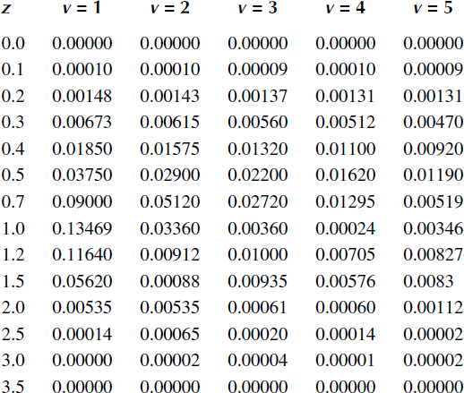
FIGURE 14.5 Maximal value of σ{F*(x)} as a function of p. Rayleigh stochastic process.

The root-mean-square deviation σ{F*(x)} of measurements of the probability distribution function of Rayleigh stochastic process as a function of the normalized level z for various values of p is presented in Figure 14.5. As we can see from Figure 14.5, the maximal value of σ{F*(x)} = 0.5 is obtained about the point z = 0.83.

The root-mean-square deviation σ{F*(x)} at z = 1 as a function of the normalized observation interval p is shown in Figure 14.6. Based on Figure 14.6 and (14.89), we can conclude that starting from p ≥ 10, in the case of Rayleigh stochastic process, the root-mean-square deviation σ{F*(x)} is inversely proportional to the ratio p = T/τ_cor. In discrete case, when the sample size is equal to N, the variance of the probability distribution function estimations F*(x) of Rayleigh stochastic process in accordance with (14.41) and (14.80) can be presented in the following form:

$Var {F^{*} (x)} = \frac{1}{N} \exp {- \frac{x^{2}}{2 σ^{2}}} {1 - \exp {- \frac{x^{2}}{2 σ^{2}}}} + {\sum^{}}_{v = 1}^{\infty} d_{v}^{'} b_{v}, (14.90)$

where

$d_{v}^{'} = \frac{2}{N} {\sum^{}}_{k = 1}^{N - 1} (1 - \frac{k}{N}) ℛ^{2 v} (k T_{p}) . (14.91)$

Applied to the Rayleigh stochastic process with uncorrelated samples, we obtain

$Var {F^{*} (x)} = \frac{1}{N} \exp {- \frac{x^{2}}{2 σ^{2}}} {1 - \exp {- \frac{x^{2}}{2 σ^{2}}}} . (14.92)$

Images

FIGURE 14.6 σ{F*(x)} as a function of the normalized observation interval p. Rayleigh stochastic process.

TABLE 14.4
Normalized Correlation Function (14.68) as a Function of the Level z

Images

Table 14.4 represents the normalized correlation function given by (14.68) in the case of probability distribution function estimation F*(x) of Rayleigh stochastic process at different values of the level z under investigations by independent samples (14.67).

14.4 Characteristics of the Probability Density Function Estimate

Determine the bias and variance of the pdf estimate of ergodic stochastic process based on an investigation of the continuous realization x(t) within the limits of the observation interval [0, T] in accordance with (14.25). Deviation of the measured pdf p*(x) from the true value p(x) can be presented in the following form:

$Δ p (x) = p^{*} (x) - p (x) = \frac{1}{T Δ x} {\int^{}}_{0}^{T} χ (t) d t - p (x), (14.93)$

where

χ(t) is given by (14.23)
Δx is the interval between the adjacent levels x_k and x_k+1

$x = \frac{x_{k} + x_{k + 1}}{2} . (14.94)$

In other words, the pdf is measured at the point corresponding to the middle of adjacent fixed levels.

The bias of the pdf estimate of ergodic stochastic process can be presented in the following form:

$b {p^{*} (x)} = \frac{1}{T Δ x} {\int^{}}_{0}^{T} 〈 χ (t) 〉 d t - p (x) . (14.95)$

The average value by realizations 〈(χt)〉 is the probability of the event that the investigated stochastic process is within the limits of the interval x ± 0.5Δx, i.e.,

$〈 χ (t) 〉 = {\int^{}}_{x - 0.5 Δ x}^{x + 0.5 Δ x} p (x) d x = F (x + 0.5 Δ x) - F (x - 0.5 Δ x) . (14.96)$

Based on (14.95) and (14.96), we are able to define the bias of the pdf estimate of ergodic stochastic process

$b {p^{*} (x)} = \frac{1}{Δ x} [F (x + 0.5 Δ x) - F (x - 0.5 Δ x)] - p (x) . (14.97)$

We can use the Taylor series expansion for the functions F(x + 0.5Δx) and F(x − 0.5Δx) about the point x:

$F (x + 0.5 Δ x) = {\sum^{}}_{μ = 0}^{\infty} \frac{d F^{μ} (x)}{d x^{μ}} \frac{1}{μ!} {(0.5 Δ x)}^{μ}; (14.98)$

$F (x - 0.5 Δ x) = {\sum^{}}_{μ = 0}^{\infty} \frac{d F^{μ} (x)}{d x^{μ}} \frac{{(- 1)}^{μ}}{μ!} {(0.5 Δ x)}^{μ} . (14.99)$

The bias of the pdf estimate of stochastic process can be presented in the following form:

$b {p^{*} (x)} = {\sum^{}}_{μ = 1}^{\infty} \frac{d^{2 μ + 1} F (x)}{d x^{2 μ + 1}} \times \frac{{(0.5 Δ x)}^{2 μ}}{(2 μ + 1)!} . (14.100)$

In practice, we can use the following approximation:

$b {p^{*} (x)} \approx \frac{Δ x^{2}}{24} \times \frac{d^{2} p (x)}{d x^{2}} + \frac{Δ x^{4}}{1920} \times \frac{d^{4} p (x)}{d x^{4}} . (14.101)$

As we can see from (14.97) through (14.101), the bias of the pdf estimate of stochastic process decreases proportionally to a decrease in the interval Δx between two adjacent fixed levels. It is clear from the physical viewpoint. In the limiting case, as Δx → 0, the bias of the pdf estimate of stochastic process tends to approach zero. In other words, as Δx → 0, the pdf estimate of stochastic process is unbiased. Actually, as Δx → 0

$\lim_{Δ x \to 0} \frac{F (x + 0.5 Δ x) - F (x - 0.5 Δ x)}{Δ x} - p (x) = \frac{d F (x)}{d x} - p (x) = 0. (14.102)$

With a decrease in the interval Δx, the variance of the pdf estimate of stochastic process increases since with a decrease in the interval Δx we observe a high deviation of total time values of stochastic process within the limits of the interval Δx from realization to realization.

Apply (14.100) to the Gaussian and Rayleigh stochastic processes. Since

$\frac{d^{v} {1 - Q (x / σ)}}{d x^{v}} = \frac{1 - Q^{v} (z)}{σ^{0.5 v}}, (14.103)$

where

$z = \frac{x}{σ}, (14.104)$

the bias of the pdf estimate of Gaussian stochastic process takes the following form:

$\begin{array}{l} = \\ \begin{array}{l} b {p^{*} (x)} & = \frac{1}{σ} {\sum^{}}_{v = 1}^{\infty} \frac{{Δ x / 2 σ}^{2 v}}{(2 v + 1)!} {1 - Q^{2 v + 1} (\frac{x}{σ})} \\ \approx \frac{1}{σ} {\frac{{Δ x / 0}^{2}}{24} {1 - Q^{3} (\frac{x}{σ})} + \frac{{Δ x / σ}^{4}}{1920} {1 - Q^{5} (\frac{x}{σ})} . \end{array} \end{array} (14.105)$

The minimal bias under the condition

$\frac{Δ x}{σ} < 1 (14.106)$

corresponds to the value z ≈ 1 at which Q³(z) ≈ 0.

Applied to the Rayleigh stochastic process, at the first approximation the bias of the pdf estimate of the Rayleigh stochastic process (the first term in (14.101)) can be presented in the following form:

$b {p^{*} (x)} \approx \frac{{(Δ x)}^{2} / σ^{2}}{24 σ} (x^{2} σ^{- 2} - 3) x σ^{- 1} \exp {- \frac{x^{2}}{2 σ^{2}}} . (14.107)$

The relative bias

$\frac{| b {p^{*} (x)} |}{p (x)} (14.108)$

of the pdf estimates of Gaussian (the solid line) and Rayleigh (the dashed line) stochastic processes as a function of the normalized interval

$Δ z = \frac{Δ x}{σ}$

at various values of the normalized level z are shown in Figure 14.7. As we can see from Figure 14.7, the relative bias of pdf estimate does not exceed the level 0.03 at Δz ≤ 0.5, which is acceptable in practice.

Images

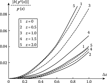
FIGURE 14.7 Relative bias of pdf estimate versus the normalized observation interval p.

Determine the variance of the pdf estimate of stochastic process. According to (14.25), we can write

$Var {p^{*} (x)} = \frac{1}{T^{2} {(Δ x)}^{2}} {\int^{}}_{0}^{T} {\int^{}}_{0}^{T} 〈 χ (t_{1}) χ (t_{2}) 〉 d t_{1} d t_{2} - {\frac{1}{T Δ x} {\int^{}}_{0 T}^{T} 〈 χ (t) 〉 d t}^{2}, (14.109)$

where

$\begin{array}{l} 〈 χ (t_{1}) χ (t_{2}) 〉 = {\int^{}}_{x - 0.5 Δ x}^{x + 0.5 Δ x} {\int^{}}_{x - 0.5 Δ x}^{x + 0.5 Δ x} f (x_{1}^{'}, x_{2}^{'}; t_{1}, t_{2}) d x_{1}^{'} d x_{2}^{'} \equiv P (x \pm 0.5 Δ x; t_{1}, t_{2}) \end{array} (14.110)$

is the probability of the event that the stochastic process ξ(t) lies within the limits of the interval x ± 0.5Δx at the instants t₁ and t₂. In the case of stationary stochastic process, the following condition is satisfied:

$P (x \pm 0.5 Δ x; τ) = P (x \pm 0.5 Δ x; - τ), (14.111)$

where τ = t₂ − t₁. By introducing new variables τ = t₂ − t₁ and t = t₁, the double integral in (14.109) is transformed into a single integral, i.e., we obtain

$Var {p^{*} (x)} = \frac{2}{T {(Δ κ)}^{2}} {\int^{}}_{0}^{T} (1 - \frac{τ}{T}) P (x \pm 0.5 Δ x) d τ - {(〈 p^{*} (x) 〉)}^{2} . (14.112)$

In practice, at the first approximation, we can suppose that the one- and two-dimensional pdfs are constant within the limits of the interval x ± 0.5Δx. Then 〈p*(x)〉 ≈ p(x) and

$P (x \pm 0.5 Δ x; τ) \approx p_{2} (x, x; τ) \times {(Δ x)}^{2} . (14.113)$

In this case, the variance of probability density function estimate of stochastic process can be presented as

$Var {p^{*} (x)} \approx \frac{2}{T} {\int^{}}_{0}^{T} (1 - \frac{τ}{T}) p_{2} (x, x; τ) d τ - p^{2} (x) . (14.114)$

In the case of Gaussian and Rayleigh stochastic processes, the two-dimensional pdfs are given by (14.50) and (14.71), respectively.

In the case of discrete stochastic process, in accordance with (14.26) the variance of the pdf estimate can be presented in the following form:

$Var {p^{*} (x)} = \frac{1}{N^{2} {(Δ x)}^{2}} {\sum^{}}_{i = 1, j = 1}^{N} 〈 χ_{i} χ_{j} 〉 - {\frac{1}{N Δ x} {\sum^{}}_{i = 1}^{N} 〈 χ_{j} 〉}^{2}, (14.115)$

where 〈χ_i χ_j〉 is given by (14.110). When the stochastic process samples are uncorrelated, we can write

$〈 χ_{i} χ_{j} 〉 = {\begin{array}{l} 〈 χ_{i} 〉 & at & i = j, \\ 〈 χ_{i} 〉 〈 χ_{j} 〉 & at & i = j . \end{array} (14.116)$

As a result, the variance of the pdf estimate of stochastic process takes the following form:

$Var {p^{*} (x)} = \frac{[F (x + 0.5 Δ x) - F (x - 0.5 Δ x)] [1 - F (x + 0.5 Δ x) + F (x - 0.5 Δ x)]}{N {(Δ x)}^{2}} . (14.117)$

Applying the Taylor series expansion for the function F(x ± 0.5Δx) about the point x and limiting by the first three terms, we obtain

$Var {p^{*} (x)} \approx \frac{p (x)}{N Δ x} [1 - Δ x p (x)] . (14.118)$

For the considered Δx, we have the following restriction p(x)Δx < 1. As we can see from (14.118), with an increase in the interval Δx the variance of the pdf estimate of stochastic process is decreased, which is confirmed by physical representation.

As applied to the Gaussian stochastic process, the variance of the pdf estimate of stochastic process defined by uncorrelated samples can be presented in the following form:

$Var {p^{*} (x)} = \frac{[Q (z - 0.5 Δ z) - Q (z + 0.5 Δ z)] {[Q (z - 0.5 Δ z) - Q (z + 0.5 Δ z)]}^{2}}{N (Δ z) σ^{2}} . (14.119)$

The dependences $\sqrt{Var {p^{*} (x)} N} / p (x)$ versus the normalized interval between the levels Δz and various values of the normalized level z under investigation of the Gaussian (the solid line) and Rayleigh (the dashed line) stochastic processes in the case of uncorrelated samples are shown in Figure 14.8.

Images

FIGURE 14.8 $\sqrt{Var {p^{*} (x)} N} / p (x)$ versus the normalized interval between the levels Δz.

Images

FIGURE 14.9 Normalized error of pdf measurement versus the normalized interval between the levels Δz.

As we can see from Figure 14.8, as opposed to the bias of the pdf estimate, the variance is decreased with an increase in the interval between levels. However, under experimental measurement of the pdf the interval between the levels Δx must be defined based on the condition of minimization of dispersion of the pdf estimate, namely,

$D {p^{*} (x)} = Var {p^{*} (x)} + b^{2} {p^{*} (x)} . (14.120)$

The normalized resulting errors of measurement of the pdf of Gaussian stochastic process $\sqrt{D {p^{*} (x)}} / p (x)$ as a function of the normalized interval between levels Δz at z = 0 and N = 10⁴ and N = 10⁵ are shown in Figure 14.9. As we can see from Figure 14.9, for the given number of samples and at z = 0, the minimal magnitude of the resulting error is decreased with a decrease in the values Δz under an increase in the number of samples.

14.5 Probability Density Function Estimate Based on Expansion in Series Coefficient Estimations

The one-dimensional stochastic process pdf can be presented in the form of series using the previously given orthogonal functions φ(x) [2]:

$p (x) = {\sum^{}}_{k = 1}^{\infty} c_{k} φ_{k} (x), (14.121)$

where the unknown coefficients are determined as

$c_{k} = \int_{- \infty}^{\infty} φ_{k} (x) p (x) d x . (14.122)$

In the case of normalized orthogonal functions, we can use the following relations:

$\int_{- \infty}^{\infty} φ_{k} (x) φ_{l} (x) d x = δ_{k l} = {\begin{array}{l} 1, & k = l; \\ 0, & k \neq l . \end{array} (14.123)$

Practically, the number of terms in expansion in series given by (14.121) is limited by some value v. Therefore, under approximation of the pdf by expansion in series, we will have forever an error

$ε (x) = p (x) - {\sum^{}}_{k = 1}^{v} c_{k} φ_{k} (x) (14.124)$

that can be reduced to the given negligible value under the corresponding choice of the orthogonal functions φ_k(x) and the number of expansions in series terms.

Further, it is convenient to characterize the approximation accuracy by the root-mean-square deviation from the true value of the pdf p(x) for all possible values of the argument x

$ε^{2} = \int_{- \infty}^{\infty} ε^{2} (x) d x = {\int_{- \infty}^{\infty} {p (x) - {\sum^{}}_{k = 1}^{v} c_{k} φ_{k} (x)}}^{2} d x . (14.125)$

Taking into consideration (14.122) and (14.123), the formula (14.125) takes the following form:

$ε^{2} = \int_{- \infty}^{\infty} p^{2} (x) d x - {\sum^{}}_{k = 1}^{v} c_{k}^{2} . (14.126)$

As we can see from the definition, the coefficients c_k of expansion in series represent, in general, the mathematical expectations of random variables subjected to the nonlinear transformation φ_k(x). As applied to ergodic stochastic process, the coefficients c_k can be defined by averaging the realization of stochastic process φ_k[x(t)] transformed in time (continuously or discretely). Taking into consideration these statements, the method to measure the pdf based on generation of orthogonal functions and estimation of coefficients of expansion in series of measured pdf was supposed in Ref. [3].

The estimate of the pdf p*(x) can be presented in the following form:

$p^{*} (x) = {\sum^{}}_{k = 1}^{v} c_{k}^{*} φ_{k} (x), (14.127)$

where the estimations of coefficients $c_{k}^{*}$ in the cases of continuous and discrete methods of investigation of the realization x(t) can be presented in the following form:

$c_{k}^{*} = \frac{1}{T} {\int^{}}_{0}^{T} φ_{k} [x (t)] d t; (14.128)$

$c_{k}^{*} = \frac{1}{N} {\sum^{}}_{i = 1}^{N} φ_{k} (x_{i}), (14.129)$

where T and N are the observation time and number of samples, respectively.

A flowchart of the considered pdf measurer functioning in real time is shown in Figure 14.10. At the measurer output, the pdf estimate is formed as a function of time

$p^{*} (t) = {\sum^{}}_{k = 1}^{v} c_{k}^{*} φ_{k} (t) . (14.130)$

Images

FIGURE 14.10 Measurer of pdf.

The measurer operates in the following way. The input realization x(t) of the stochastic process is subjected to multichannel inertialess transformation φ[x(t)] and is averaged after that by ideal integrators. As a result, the estimations of the expansion in series coefficients $c_{k}^{*}$ are formed. These coefficients $c_{k}^{*}$ come in at the mixer inputs. The orthogonal functions of time %(t) come in at the second mixer input. The estimate of the pdf p*(t) as a function of time is formed at the summator output. The orthogonal time functions φ_k(t) coming at the mixers are delayed on the time T. This time is required to obtain the estimations of coefficients $c_{k}^{*}$ .

Determine the characteristics of the pdf estimations. Sinc

$〈 φ_{k} [x (t)] 〉 = \int_{- \infty}^{\infty} φ_{k} (x) p (x) d x, (14.131)$

we can see from (14.128) and (14.129) that the estimations of coefficients $c_{k}^{*}$ are unbiased, i.e.,

$〈 c_{k}^{*} 〉 = c_{k} . (14.132)$

The resulting dispersion of the pdf estimate can be presented in the following form:

$D {p^{*}} = 〈 \int_{- \infty}^{\infty} {[p (x) - p^{*} (x)]}^{2} d x 〉 = ε^{2} + {\sum^{}}_{k = 1}^{v} [〈 c_{k}^{*^{2}} 〉 - c_{k}^{2}] . (14.133)$

The second term

$Var {p^{*}} = {\sum^{}}_{k = 1}^{v} [〈 c_{k}^{*^{2}} 〉 - c_{k}^{2}] (14.134)$

is the variance of the pdf estimate caused by random errors under estimation of the coefficients $c_{k}^{*}$ .

Determine the second initial moment of the coefficient of expansion in series applied to the continuous method given by (14.128). We obtain

$〈 c_{k}^{*^{2}} 〉 = \frac{1}{T^{2}} {\int^{}}_{0}^{T} {\int^{}}_{0}^{T} 〈 φ_{k} [x (t_{1})] φ_{k} [x (t_{2})] 〉 d t_{1} d t_{2} . (14.135)$

The mathematical expectation of the integrand can be presented in the following form:

$〈 φ_{k} [x (t_{1})] φ_{k} [x (t_{2})] 〉 〉 = \int_{- \infty}^{\infty} \int_{- \infty}^{\infty} φ_{k} (x_{1}) φ_{k} (x_{2}) p_{2} (x_{1}, x_{2}; τ) d x_{1} d x_{2} = Ψ (τ = | t_{2} - t_{1} |), (14.136)$

where p₂(x₁, x₂; τ) is the two-dimensional pdf of the investigated stochastic process. Substituting (14.136) into (14.135), introducing new variables τ = t₂ − t₁ and t = t₁, and changing the order of integration, we obtain

$〈 c_{k}^{* 2} 〉 = \frac{2}{T} {\int^{}}_{0}^{T} (1 - \frac{τ}{T}) Ψ (τ) d τ . (14.137)$

As applied to investigation of stochastic process realization at discrete instants

$〈 c_{k}^{* 2} 〉 = \frac{1}{N^{2}} {\sum^{}}_{i = 1}^{N} {\sum^{}}_{j = 1}^{N} 〈 φ_{k} (x_{i}) φ_{k} (x_{j}) 〉, (14.138)$

where 〈φ_k(x_i)φ_k(x_j)〉 is defined by analogous way as in (14.136).

Under analysis of stochastic process realizations at independent instants, the components

$Δ φ_{k} (x_{i}) = φ_{k} (x_{i}) - c_{k} (14.139)$

will be independent random variables. Therefore, the mathematical expectation of the square of the estimate of the expansion in series coefficients $〈 c_{k}^{*^{2}} 〉$ given by (14.138) can be presented in the following form:

$〈 c_{k}^{*^{2}} 〉 = c_{k}^{2} + \frac{1}{N^{2}} {\sum^{}}_{i = 1}^{N} 〈 Δ φ_{k}^{2} (x_{i}) 〉 . (14.140)$

The variance of random component Δφ_k(x_i) is defined by the well-known relationship

$Var {Δ φ_{k}} = 〈 Δ φ_{k}^{2} (x_{j}) 〉 = \int_{- \infty}^{\infty} {[φ_{k} (x) - c_{k}]}^{2} p (x) d x (14.141)$

and does not depend on the number of sample. Because of this, we can write the variance of the pdf estimate in the following form:

$Var {p^{*}} = \frac{1}{N} {\sum^{}}_{k = 1}^{v} Var {Δ φ_{k}} . (14.142)$

As we can see from (14.142), the variance of the pdf estimate is decreased with an increase in the number of independent samples and is increased with an increase in the number of expansion in series terms v. Since the approximation accuracy is also increased with increasing the number of expansion in series terms, under approximation of the measured pdf by expansion in series, the number of terms must be chosen based on the condition of minimization of estimate dispersion:

$D {p^{*}} = \int_{- \infty}^{\infty} p^{2} (x) d x - {\sum^{}}_{k = 1}^{v} c_{k}^{2} + \frac{1}{N} {\sum^{}}_{k = 1}^{v} Var {Δ φ_{k}} . (14.143)$

In practice, to design and construct the digital or analog measurer of the pdf, the non-normalized orthogonal functions of threshold type can be chosen as the functions φ_k(x), i.e.,

$φ_{k} (x) = {\begin{array}{l} 1 & if & x_{k} \leq x \leq x_{k + 1}, \\ 0 & if & x < x_{k}, x > x_{k + 1} . \end{array} (14.144)$

In this case, the coefficients of expansion in series are defined in the following form:

$c_{k} = \frac{{\int_{x_{k}}^{x_{k + 1}} φ_{k} (x) p (x) d x}^{}}{\int_{x_{k}}^{x_{k + 1}} φ_{k}^{2} (x) d x} = \frac{Δ F_{k}}{Δ x_{k}}, (14.145)$

where

$Δ F_{k} = F (x_{k + 1}) - F (x_{k}) (14.146)$

is the probability of the event that the realizations of stochastic process lie within the limits of the interval Δx_k = x_k+1 − x_k of argument x. Formula (14.145) is obtained by multiplication of the left and right parts of (14.121) on φ_k(x), integration with respect to x within the limits from x_k to x_k+1 and taking into consideration the condition of orthogonality. For the orthogonal functions given by (14.144) the coefficients c_k are the ordinates of the approximated pdf and look like the discrete curve shown in Figure 14.11. It is easy to see that the coefficient estimations are unbiased.

Images

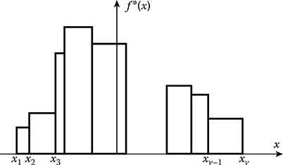
FIGURE 14.11 Histogram of distribution.

As applied to discrete sampling, in the considered case, the coefficient estimations of expansion in series can be presented in the following form:

$c_{k}^{*} = \frac{1}{Δ x_{k}} \times \frac{1}{N} {\sum^{}}_{i = 1}^{N} φ_{k} (x_{j}) . (14.147)$

In the case of an independent sample of stochastic process, the variance of estimations of stochastic components φ_k(x_i) can be presented in the following form:

$Var {Δ φ_{k}} = {\int^{}}_{x_{k}}^{x_{k + 1}} φ_{k}^{2} (x) p (x) d x - {{\int^{}}_{x_{k}}^{x_{k + 1}} φ_{k} (x) p (x) d x}^{2} = Δ F_{k} (1 - Δ F_{k}) . (14.148)$

By analogous way, the variance of the pdf estimate can be presented as

$Var {p^{*}} = \frac{1}{N} {\sum^{}}_{k = 1}^{v} \frac{Var {Δ φ_{k}}}{Δ x_{k}^{2}} = \frac{1}{N} {\sum^{}}_{k = 1}^{v} \frac{Δ F_{k} (1 - Δ F_{k})}{Δ x_{k}^{2}} . (14.149)$

If the interval between samples is constant, i.e., Δx_k = Δx = const, then

$Var {p^{*}} = \frac{1}{N Δ x^{2}} {\sum^{}}_{k = 1}^{v} Δ F_{k} (1 - Δ F_{k}) = {\sum^{}}_{k = 1}^{v} Var {p^{*} (x_{k})}, (14.150)$

where Var{p*(x_k)} coincides with (14.117) for the level x_k, as expected.

14.6 Measurers of Probability Distribution and Density Functions: Desig Nprinciples

Under practical realization of measurers of the stochastic process pdf, the multichannel amplitude analyzers are widely used. The number of channels is very high and can be more than 1024 or 4096 channels. As applied to investigation of continuous stochastic process, the input realization x(t) is transformed into a sequence of pulses, the duration of which is much less than the correlation interval of stochastic process and the pulse amplitude corresponds to instantaneous value of the input realization of stochastic process. In doing so, a range of possible values of the input realization x(t) of stochastic process should with high probability be within the limits of the interval [c, d] defined by the multichannel analyzer. As a rule, the range of possible values [c, d] is divided by v equal intervals with the width given as

$Δ x = \frac{d - c}{v} . (14.151)$

Giving the total number of pulses (samples) by N and measuring the number of pulses N_j at the jth channel, the pdf estimate can be presented by analogy with (14.26)

$p_{j}^{*} (x) = \frac{N_{j}}{N Δ x} = \frac{N_{j}}{N} \times \frac{v}{d - c} . (14.152)$

Images

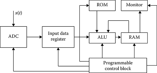
FIGURE 14.12 Measurer of pdf.

The upper bound of the jth channel can be presented in the following form:

$\begin{matrix} g_{j} = c + j Δ x, & j = 1, 2, ..., v . \end{matrix} (14.153)$

As a result, we obtain the estimations of ordinate of the stochastic process pdf at the points

$x_{j} = \frac{c + Δ x (2 j - 1)}{2} (14.154)$

corresponding to the middle between the levels g_j and g_j−1.

The principal flowchart of a pdf measurer is shown in Figure 14.12. The functioning principles are the following. The input realization x(t) of a stochastic process comes in at the ADC input. After sampling in time and amplitude, the input signal comes in at the input of input data register and, after that, at the ALU input, in which a determination of the pdf is carried out according to algorithm. The final result, i.e., the ALU output, changes information in RAM for output data, where the values of probability density function estimates for all ν channels are stored. The value of the pdf is reproduced by a monitor. Initial data required to compute the pdf estimations are stored by ROM in the form of total number of samples N, interval between the channels (or levels) Δx, and interval [c, d] of possible values of investigated stochastic process. The channel number where we can find the reading x[i] = x_i can be defined as

$j = {\frac{x [i] - c}{Δ x}} + 1, (14.155)$

where {…}.means the integer number. The algorithm to compute the pdf estimate is presented in Figure 14.13. There is a need to note that all blocks of the structural block diagram can be realized by microprocessor systems.

The previously mentioned methods to measure the pdf are based on uniform division of the range of possible stochastic process values. However, this procedure, as a rule, is not optimal, since peculiarities of measured characteristic variations are not taken into consideration, which leads finally to information excess and high errors under definition of characteristics of argument values. Additionally, there is an inverse problem—to define the argument values by the given pdf values.

Consider the method of argument definition by the given characteristic values applied to the probability distribution function estimate in the case of sampled stochastic process. Division of probability distribution function domain on discrete values F_j must be done in accordance with the applied problem. The most favorable action is a uniform division from zero to unit using the equal intervals δF. The method to define an argument of probability distribution function is the following. In the case of arbitrary argument, according to the rule given by (14.20), the probability distribution function estimate F*(x) is computed and compared with the given value F_j. As a result of comparison, we obtain the signal

Images

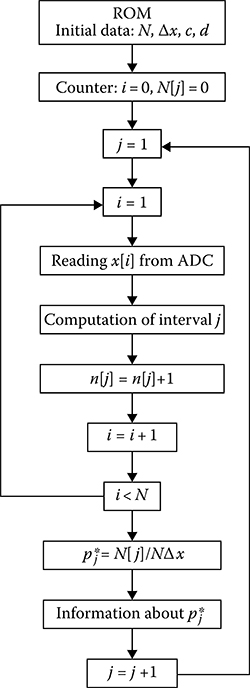
FIGURE 14.13 Algorithm of pdf computation.

$ε (x) = F_{j} - F^{*} (x), (14.156)$

based on which it is possible to measure the level x. The value $x_{j}^{*}$ at which the signal given by (14.156) is equal to zero is the estimate of probability distribution function argument. In practice, a nonzero measure is chosen as a criterion that the estimate F*(x) is very close to F_j. The simplest way to define this measure is to compare the module of the signal given by (14.165) with the previously given value ε. In this case, the level satisfying the condition

$| ε (x) | \leq ε . (14.157)$

can be considered as the estimate $x_{j}^{*}$ . The probability distribution function can be given either in the form of deterministic numbers F_j within the limits of the interval [0,1] or using the values of corresponding transformations of reference stochastic process samples with the known probability distribution function [4].

Consider the measurement method when the probability distribution function is given as a set of discrete numbers F_j. In this case, the current estimate $x_{j}^{*}$ of argument for jth value of probability distribution function can be defined using the recurrent relationship (12.342) that can be transformed and applied to the considered method of measurement in the following form:

$x_{j}^{*} [N] = x_{j}^{*} [N - 1] + γ [N] {F_{j} - F_{j}^{*} [N]} . (14.158)$

In doing so, the current estimate of the probability distribution function $F_{j}^{*} [N]$ at the nth step is defined as

$F_{j}^{*} [N] = \frac{1}{N} {\sum^{}}_{i = 1}^{N} η_{x} [i], (14.159)$

where we use the transformation by analogy with (14.19)

$η_{x} [i] = {\begin{array}{l} 1 & if & x [i] \leq x_{j}^{*} [i - 1], \\ 0 & if & x [i] > x_{j}^{*} [i - 1] . \end{array} (14.160)$

Transformation (14.160) means that the current sample of investigated stochastic process at the ith iteration step is compared with the argument estimate obtained at the previous (i − 1)th iteration step. Initial argument value $x_{j}^{*} [0] = a$ is chosen in arbitrary way from the range of possible values [c, d]. The factor γ[N] defining the next iteration step must satisfy the condition given by (12.343). As a rule, it is inversely proportional to the number of iterations, i.e., γ[N] = κN⁻¹, where κ > 0 characterizes the value of the first iteration step. The probability distribution function estimate given by (14.159), by analogous way with (12.347), can be presented in the following form:

$F_{j}^{*} [N] = F_{j}^{*} [N - 1] + N^{- 1} {η_{x} [N] - F_{j}^{*} [N - 1]} . (14.161)$

The iteration number N is defined based on the selected rule. The most widely used rule can be presented in the following form:

$| x_{j}^{*} [N] - x_{j}^{*} [N - 1] | = α [N] \leq α, (14.162)$

where α > 0 is the given number. When the condition (14.162) is satisfied, the iteration process is stopped. The structure of algorithm to compute the argument estimates for the given values of probability function distribution is shown in Figure 14.14.

Computing a ratio of the end differences of probability distribution function and its arguments, we can define the pdf estimate of the investigated stochastic process. As applied to the probability distribution function estimate by three of its values $x_{j - 1}^{*}$ , $x_{j}^{*}$ , and $x_{j + 1}^{*}$ , the pdf estimate for the argument $x_{j}^{*}$ can be presented in the following form:

$p_{j}^{*} (x) = \frac{1}{2} {\frac{F_{j} - F_{j - 1}}{x_{j}^{*} - x_{j - 1}^{*}} + \frac{F_{j + 1} - F_{j}}{x_{j + 1}^{*} - x_{j}^{*}}} . (14.163)$

Images

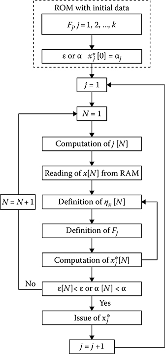
FIGURE 14.14 Algorithm of the argument estimate computation.

Under the use of reference stochastic process with the known pdf, the structure of algorithm to measure the arguments of probability distribution function is changed. Denote discrete values of realizations of investigated and reference stochastic processes as x_i and y_i, respectively. As applied to the reference stochastic process, we can theoretically define the argument value y by the given value of probability distribution function F(y) = F_j. If we apply the following transformation

$η_{y i} = {\begin{array}{l} 1 & if & y_{i} \leq y, \\ 0 & if & y_{i} > y, \end{array} (14.164)$

with respect to samples y_i of reference stochastic process, then the unbiased probability distribution function estimate F*(y) of random sample y_i is defined by (14.20). Comparing the probability distribution function estimate of reference stochastic process with the probability distribution function estimate F*(x) of the investigated stochastic process, we obtain the signal

$ε (x) = F^{*} (y) - F^{*} (x) = \frac{1}{N} {\sum^{}}_{i = 1}^{N} z_{i}, (14.165)$

where z_i = η_yi − η_xi takes the following values:

$z_{i} = {\begin{array}{l} 1 & if & x_{i} \leq x, y_{i} > y, \\ 0 & if & {\begin{matrix} x_{i} > x, y_{i} > y, \\ x_{i} \leq x, y_{i} \leq y, \end{matrix} \\ - 1 & if & x_{i} > x, y_{i} \leq y . \end{array} (14.166)$

Varying the level x at which the signal ε(x) given by (14.165) can satisfy (14.157), we obtain the argument estimate $x_{j}^{*}$ for the probability distribution function F_j. The argument estimate $x_{j}^{*}$ for the probability distribution function F_j can be found by an iteration procedure based on recurrent relationship [4]:

$x_{j}^{*} [N] = x_{j}^{*} [N - 1] + γ [N] z [N] . (14.167)$

Part of the flowchart of the digital measurer of the probability distribution function arguments employing the sensors of reference random numbers is presented in Figure 14.15. Operation of ROM and corresponding programmable blocks is identical to functions of the measurer of pdf (see Figure 14.12). ALU must define the end of iteration procedure according to (14.157) or (14.162). The algorithm to compute the argument estimations of probability distribution function is presented in Figure 14.16. This algorithm is different from the algorithm presented in Figure 14.14. The difference is that the arguments y_i, j = 1, 2,…, k corresponding to known values of the probability distribution function of reference stochastic process (RSP) are given instead of probability distribution function F_j values.

The procedure for the measurement of probability distribution function arguments allows us to define the required number N of iterations based on the given relative root-mean-square deviation of the probability distribution function estimate. The disadvantage of such a measurer is the presence of transient process under definition of argument estimate $x_{j}^{*}$ . The considered procedures and methods of measurements of probability distribution functions and pdfs are acceptable in the case of pulse stochastic processes. In this case, the software control device and ADC must be synchronized by the investigated pulse stochastic process.

Images

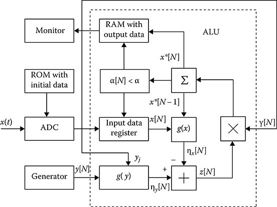
FIGURE 14.15 Measurer of probability distribution function argument.

Images

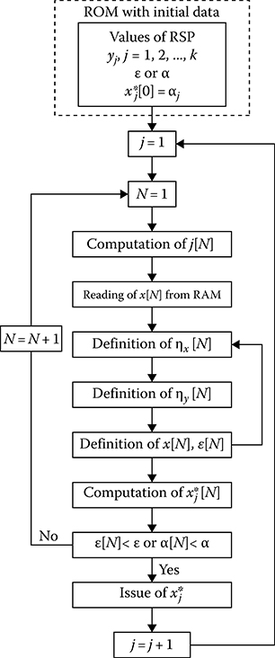
FIGURE 14.16 Algorithm of computation of the probability distribution function argument estimations.

14.7 Summary and Discussion

The pdf is defined experimentally like the average value of the pdf within the limits of the interval [x ± 0.5dx]. Because of this, from the viewpoint of approximation of the measured pdf to its true value at the level x, it is desirable to decrease the interval Δx. However, a decrease in the Δx at the fixed observation time interval leads to a decrease in time of the stochastic process within the limits of the interval Δx and, consequently, to an increase in the variance of the pdf estimate owing to decreasing the statistical data sample based on which the decision about the pdf magnitude is made. Therefore, there is an optimal value of the interval Δx, under which the dispersion of the pdf estimate takes the minimal magnitude at the fixed observation time.

There are several ways to measure the total time of a stochastic process observation below the given level or within its limits. The first way is the direct measurement of total time when a magnitude of the realization of continuous ergodic process is below the fixed level x. In this case, the realization of continuous ergodic process is transformed into the sequence of rectangular pulses (see the Figure 14.1b) with the unit amplitude and duration equal to the time when a magnitude of the realization of continuous ergodic process is below the fixed level. The second method to define and measure the probability distribution function is based on computation of the number of quantized by amplitude and duration of the sampled pulses. In this case, at first, the continuous realization of stochastic process is transformed by corresponding pulse modulator into sampled sequence and comes in at the input of the threshold device with the threshold level. Then, a ratio of the number of pulses that do not exceed the threshold to the total number of pulses corresponding to the observation time interval is equal by value to the probability distribution function estimate.

The root-mean-square deviation σ{F*(x)} of measurements of the probability distribution function of Gaussian stochastic process as a function of the normalized level for various values of p is presented in Figure 14.3. As we can see from Figure 14.3, the maximal values of σ{F*(x)} are obtained at the zero level. Formula (14.63) demonstrates that the variance of the probability distribution function estimate F*(x) of stochastic process by correlated samples increases in comparison with the variance of the probability distribution function estimate F*(x) of stochastic process by uncorrelated samples of the same sample size N.

The dependences $\sqrt{Var {f^{*} (x)} N} / p (x)$ versus the normalized interval between the levels Δz and various values of the normalized level z under investigation of the Gaussian (the solid line) and Rayleigh (the dashed line) stochastic processes in the case of uncorrelated samples are shown in Figure 14.8. As we can see from Figure 14.8, as opposed to the bias of pdf estimate, the variance of the pdf estimate is decreased with an increase in the interval between levels. However, under experimental measurement of the pdf the interval between the levels Δx must be defined based on the condition of minimization of dispersion of the pdf estimate. The normalized resulting errors of measurement of the probability density function of Gaussian stochastic process $\sqrt{D {p^{*} (x)}} / p (x)$ as a function of the normalized interval between levels Δz at z = 0 and N = 10⁴ and N = 10⁵ are shown in Figure 14.9. As we can see from Figure 14.9, for the given number of samples and at z = 0, the minimal magnitude of the resulting error is decreased with a decrease the values Δz under an increase in the number of samples.

REFERENCES

1. Haykin, S. and M. Moher. 2007. Introduction to Analog and Digital Communications. 2nd Edn. New York: John Wiley & Sons, Inc.

2. Gradshteyn, I. S. and I. M. Ryzhik. 2007. Tables of Integrals, Series and Products.7th Edn. London, U K.: Academic Press.

3. Sheddon, I. N. 1951. Fourier Transform. New York: McGraw Hill, Inc.

4. Domaratzkiy, A. N., Ivanov, L. N., and Yu. Yurlov. 1975. Multipurpose Statistical Analysis of Stochastic Signals. Novosibirsk, Russia: Nauka.

..................Content has been hidden....................

You can't read the all page of ebook, please click here login for view all page.

Table of Contents for
Chapter 14 Estimation of Probability Distribution and Density Functions of Stochastic Process

14 Estimation of Probability Distribution and Density Functions of Stochastic Process

14.1 Main Estimation Regularities

14.2 Characteristics of Probability Distribution Function Estimate

14.3 Variance of Probability Distribution Function Estimate

14.3.1 GAUSSIAN STOCHASTIC PROCESS

14.3.2 RAYLEIGH STOCHASTIC PROCESS

14.4 Characteristics of the Probability Density Function Estimate

14.5 Probability Density Function Estimate Based on Expansion in Series Coefficient Estimations

14.6 Measurers of Probability Distribution and Density Functions: Desig Nprinciples

14.7 Summary and Discussion

REFERENCES

Table of Contents for Chapter 14 Estimation of Probability Distribution and Density Functions of Stochastic Process

Create new playlist

Sign In

Sign Up

Table of Contents for
Chapter 14 Estimation of Probability Distribution and Density Functions of Stochastic Process