Chapter 5 Filtering and Extrapolation of Target Track Parameters Based on Radar Measure

Search in book...
Toggle Font Controls
Create new playlist

Name your new playlist

Playlist description (optional)
Sign In

Email address

Password

Forgot Password?

or

Continue with Facebook

Continue with Google
Sign Up

Full Name

Email address

Confirm Email Address

Password

or

Continue with Facebook

Continue with Google

A track represents the belief that a physical object or target is present and has actually been detected by the complex radar system (CRS). An automatic radar-tracking subsystem forms a track when enough radar detections are made in a believable enough pattern to indicate that a target is actually present (as opposed to a succession of false alarms) and when enough time has passed to allow accurate calculation of the target’s kinematics state—usually the target position and velocity. Thus, a goal of tracking is to transform a time-lapse detection picture, consisting of target detections, false alarms, and clutter, into a track picture, consisting of tracks on real targets, occasional false tracks, and occasional deviations of track position from true target positions.

When a track is established in a computer subsystem, it is assigned a track number (the track file). All parameters associated with a given track are referred to by this track number. Typical track parameters are the filtered and predicted position; velocity; acceleration (when applicable); time of last update; track quality; SNR; covariance matrices—the covariance contains the accuracy of all the track coordinates and all the statistical cross-correlations between them, if a Kalman-type filter is being used; and track history, that is, the last n detections. Tracks and detections can be accessed in various sectored, linked-list, and other data structures so that the association process can be performed efficiently. In addition to the track file, a clutter file is maintained. A clutter number is assigned to each stationary or slowly moving echo. All parameters associated with a clutter point are referred to by this clutter number. Again, each clutter number is assigned to a sector in azimuth for efficient association.

There are many sources of error in radar-tracking performance. Fortunately, most are insignificant except for high-precision tracking-radar applications such as range instrumentation, where the angle precision required may be on the order 0.05 mrad (mrad, or milliradian, is 1000th of a radian, or the angle subtended by 1 m cross-range at 1000 m range). Many sources of error can be avoided or reduced by radar design or modification of the tracking geometry. Cost is a major factor in providing high-precision-tracking capability. Therefore, it is important to know how much errors can be tolerated, which sources of error affect the application, and what are the most cost-effective means to satisfy the accuracy requirements.

Because tracking radar subsystems track targets not only in angle but also in range and sometimes in Doppler, the errors in each of these target parameters must be considered in most error budgets. It is important to recognize the actual CRS information output. For a mechanically moved antenna, the angle-tracking output is usually obtained from the shaft position of the elevation and azimuth antenna axes. Absolute target location relative to each coordinates will include the accuracy of the survey of the antenna pedestal site. Phased array instrumentation radar system, such as the multiobject tracking radar (MOTR), provides electronic beam movement over a limited sector of about ±45° to approximately ±60° plus mechanical movement of the antenna to move the coverage sector [1–4].

Radar target tracking is performed by the use of the echo signal reflected from a target illuminated by the radar transmit pulse. This is called skin tracking to differentiate it from beacon tracking, where a beacon or a transponder transmits its signal to the radar and usually provides a stronger point-source signal. Because most targets, such as aircraft, are complex in shape, the total echo signal is composed of the vector sum of a group of superimposed echo signals from the individual parts of the target, such as the engines, propellers, fuselage, and wing edges. The motions of a target with respect to the CRS cause the total echo signal to change with time, resulting in random fluctuations in the radar measurements of the parameters of the target. These fluctuations caused by the target only, excluding atmospheric effects and radar receiver noise contributions, are called the target noise. This discussion of target noise is based largely on aircraft, but it is generally applicable to any target, including land targets of complex shape that are large with respect to a wavelength. The major difference is in the target motion, but the discussions are sufficiently general to apply to any target situation.

The echo return from a complex target differs from that of a point source by the modulations that are produced by the change in amplitude and relative phase of the returns from the individual elements. The word modulations is used in plural form because five types of modulation of the echo signal that are caused by a complex target affect the CRS. These are amplitude modulation, phase front modulation (glint), polarization modulation, Doppler modulation, and pulse time modulation (range glint). The basic mechanism by which the modulations are produced is the motion of the target, including yaw, pitch, and roll, which causes the change in relative range of the various individual elements with respect to the radar. Although the target motions may appear small, a change in relative range of the parts of a target of only one-half wavelength (because of the two-way radar signal path) causes a full 360° change in relative phase.

5.1 Initial Conditions

The problem to define the estimation θˆ(ti) $\hat{θ} (t_{i})$ of target track parameters θ(t) by the observed coordinate sample Y(t_i), i = 0, 1,…, n,… is solved in all stages of signal reprocessing in a CRS. In the course of signal reprocessing, we can distinguish the following kinds of target track parameter estimations [5,6]:

Estimation obtained at the instant t_j = t_n: the last measurement, that is, target track parameter filtering
Estimation obtained at predicted coordinates at the point t_j > t_n—the extrapolation of target track parameters
Estimation obtained at the points lying within the limits of the interval of observation 0 ≤ t_j < t_n—the target track parameter smoothing

In this chapter, we discuss only the first and second problems of target track parameter estimation definition. The class of considered objects is mainly limited by air targets. There is a need to take into consideration that in this chapter we discuss only the main results of filtering theory and extrapolation methods with reference to signal reprocessing problems in CRSs. We use the representation form that is understandable to designers and engineers of signal processing algorithms, and computer architecture systems and other experts exploiting CRSs for various areas of application.

5.2 Process Representation in Filtering Subsystems

5.2.1 TARGET TRACK MODEL

In solving the filtering problems, a presentation procedure of variation of the filtered target parameters as a function of time takes a principal meaning. In our case, this corresponds to the choice of target track model. In the case of signal reprocessing problems in CRSs, taking into consideration sampling and discretization of target coordinate measuring and radio frequency interference, the target track model can be described by a system of linear difference equations that can be presented in the following vector form:

$θ_{n + 1} = Φ_{n} θ_{n} + Γ_{n} η_{n} = {θ^{'}}_{n + 1} + Γ_{n} η_{n}, (5.1)$

where

θ_n is the s-dimensional target track parameter vector at the nth step
Φ_n is the known s × s transfer matrix
η_n is the h-dimensional vector of target track parameter disturbance
Γ_n is the known s × h matrix
θ′_n+1 is the deterministic (undisturbed) component of the target track parameter vector at the (n + 1)th step

Under polynomial representation of independent target coordinates, a prediction of parameters of an undisturbed target track, for example, by target range coordinate r(t), is carried out in the following manner:

$\begin{array}{l} r_{n + 1} = r_{n} + {\dot{r}}_{n} τ_{n} + 0.5 {\ddot{r}}_{n} τ_{n}^{2} + \dots, \\ {\dot{r}}_{n + 1} = {\dot{r}}_{n} + {\ddot{r}}_{n} τ_{n} + \dots, \\ {\ddot{r}}_{n + 1} = {\ddot{r}}_{n} + {\overset{⃛}{r}}_{n} τ_{n} + \dots, \\ ............................ \end{array} (5.2)$

where

τ_n = t_n+1 − t_n; t_n and t_n+1 are the readings of the function r(t)
r_n, ${\dot{r}}_{n}$ , ${\ddot{r}}_{n}$ , … are the target track parameters representing the target track coordinate, velocity of target track coordinate variation, and acceleration by the target track coordinate

Using the vector-matrix representation in (5.2), we obtain

${θ^{'}}_{n + 1 (r)} = Φ_{n} θ_{n (r)}, (5.3)$

where

$\begin{matrix} θ_{n (r)} = ‖ \begin{matrix} r_{n} \\ {\dot{r}}_{n} \\ {\ddot{r}}_{n} \\ ⋮ \end{matrix} ‖ & and & Φ_{n} = ‖ \begin{matrix} 1 & τ_{n} & 0.5 τ_{n}^{2} & \dots \\ 0 & 1 & τ_{n} & \dots \\ 0 & 0 & 1 & \dots \\ \dots & \dots & \dots & \dots \end{matrix} ‖ \end{matrix} (5.4)$

Formulas for undisturbed target track parameters by other independent coordinates take an analogous form.

The second term in the target track model given by (5.1) must take into consideration, first of all, the target track parameter disturbance caused by the nonuniform environment in which the target moves, atmospheric conditions, and, also, inaccuracy and inertness of control and target parameter stabilization system in the course of target moving. We may term this target track parameter disturbance as the control noise, that is, the noise generated by the target control system. As a rule, the control noise is presented as the discrete white noise with zero mean and the correlation matrix defined as follows:

$E [η_{i} η_{j}^{T}] = σ_{n}^{2} δ_{i j}, (5.5)$

where

E is the mathematical expectation
$σ_{n}^{2}$ is the variance of control noise
δ_ij is the Kronecker symbol, that is, δ_ij = 1, if i = j and 0 if i ≠ j

In addition to the control noise, the target track model must take into consideration specific disturbances caused by unpredictable changes in target track parameters that are generated by target inflight maneuvering. We call these disturbances the target maneuver noise. In a general case, the target maneuver noise is neither the white noise nor the Gaussian noise. One possible example of the target maneuver noise is the pdf of target (aircraft) acceleration, the so-called target maneuver intensity, by one coordinate (see Figure 5.1), where P₀ is the probability of target maneuver absence and P₁ is the probability of target maneuver with the maximal acceleration $\pm g_{m_{\max}}$ . The probability of any intermediate value of the target maneuver intensity or the pdf of target acceleration is given by

$p = \frac{1 - (2 p_{1} + p_{0})}{2 g_{m_{\max}}} . (5.6)$

The equiprobability of intermediate values of the target maneuver intensity or the pdf of target acceleration can be founded, for example, by the fact that the projection of the target maneuver intensity by the target course (the most frequent target maneuver case) onto arbitrary direction takes a value within the limits $\pm g_{m_{\max}}$ . In the case of a set of the target maneuvers in time and space, we can believe that these values are equally probable.

Images

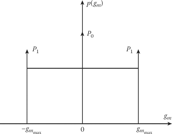
FIGURE 5.1 Example of pdf of the target maneuver intensity (acceleration).

Since performing the target maneuver requires, as a rule, so much time (in any case, more time in comparison with the time interval τ_n defined between two target coordinate measurements), the target maneuver intensity or pdf of target acceleration is correlated, at some instant of observation, with the target maneuver intensity observed previously or in succeeding instants. By this reason, we must know the autocorrelation function of the target maneuver noise to characterize it statistically. Usually, the autocorrelation function of the target maneuver intensity can be presented in exponential form as follows:

$E [g_{m} (t) g_{m} (t + τ)] = R_{m} (τ) = σ_{m}^{2} \exp (- α | τ |), (5.7)$

where

α is the value that is inversely proportional to the average duration of target maneuver T_m, that is, $α = T_{m}^{- 1}$
$σ_{m}^{2}$ is the variance of the target maneuver intensity

In the case of equivalent discrete time, the autocorrelation function of the target maneuver intensity can be presented in the following form:

$R_{m} (n) = σ_{m}^{2} \exp {- α | n T_{n e w} |} = σ_{m}^{2} ρ^{| n |} (5.8)$

where

$ρ = \exp {- α T_{n e w}}, (5.9)$

T_new is the period of getting new information about the target. Further values of the target maneuver intensity can be presented using the previous one, for example,

$g_{m_{n + 1}} = ρ g_{m_{n}} = \sqrt{σ_{m}^{2} (1 - ρ^{2})} ξ_{n}, (5.10)$

where ξ_n is the white noise with zero mean and the variance equal to unit.

In practice, in designing the CRSs, we can conditionally think that a set of targets can be divided into maneuvering and nonmaneuvering targets. The target is not considered as a maneuvering target if it moves along a straight line with the constant velocity accurate within the action of the control noise intensity. In other cases, the target is maneuvering. For example, in the case of aerodynamic objects, the nonmaneuvering target model is considered as the main model and each coordinate of this model is defined by the polynomial of the first order. However, this classification has a sense only in the case when the filtering parameters of target track are represented in the Cartesian coordinate system under signal processing in CRSs. If the filtering parameters of the target track are represented in the spherical coordinate system, then they are changed nonlinearly even when the target is moving along the straight line and uniformly. In this case, the polynomial of the second order must be applied to represent the independent target coordinates.

5.2.2 MEASURING PROCESS MODEL

In the solution of the filtering problems, in addition to the target track model there is a need to specify a function between the m-dimensional vector of measured coordinates Y_n and s-dimensional vector of estimated parameters θ_n at the instant of nth measuring. This function, as a rule, is given by a linear equation:

$Y_{n} = H_{n} θ_{n} + Δ Y_{n}, (5.11)$

where

H_n is the known m × s matrix defining a function between the observed coordinates and estimated parameters of target track
ΔY_n is the error of coordinate measuring

In the considered case, the observed coordinates are the current target coordinates in a spherical coordinate system—the target range r_n, the azimuth β_n, the elevation ε_n, or some specific coordinates for CRSs—and radar coordinates, for example, the radar range, cosine between the radar antenna array axis and direction to the target. In some CRSs, the radial velocity ${\dot{r}}_{n}$ can serve as the measured coordinate. The matrix H_n = H takes the simplest form and consists of zeros and units when the target track parameters are estimated by the observed coordinates in the spherical coordinate system. For example, if we measure the target spherical coordinates r_n, β_n, and the parameters ${\hat{r}}_{n}, \hat{\dot{r}}, β_{n}, {\hat{\dot{β}}}_{n}$ (the linear approximation) are filtered, then the matrix H_n takes the following form:

$\begin{array}{l} H_{n} = ‖ \begin{array}{l} 1 & 0 & 0 & 0 \\ 0 & 0 & 1 & 0 \end{array} ‖ \begin{matrix} \to r_{n} \\ \to β_{n} \end{matrix}) \\ \begin{matrix} \begin{matrix} \begin{array}{l} ↓ \\ {\hat{r}}_{n} \end{array} & \begin{array}{l} ↓ \\ {\hat{\dot{r}}}_{n} \end{array} & \begin{array}{l} ↓ \\ {\hat{β}}_{n} \end{array} & \begin{array}{l} ↓ \\ {\hat{\dot{β}}}_{n} \end{array} \end{matrix} \end{matrix} \end{array} (5.12)$

When the target track parameters are filtered by measured spherical coordinates in the Cartesian coordinate system, then computation of elements of the matrix H_n is carried out by differentiation of transformation formulas from the spherical coordinate system to the Cartesian one:

$\begin{array}{l} H_{n} = ‖ \begin{array}{l} \frac{d r_{n}}{d x_{n}} & 0 & \frac{d r_{n}}{d y_{n}} & 0 \\ \frac{d β_{n}}{d x_{n}} & 0 & \frac{d β}{d y_{n}} & 0 \end{array} ‖ \begin{matrix} \to r_{n} \\ \to β_{n} \end{matrix}) \\ \begin{matrix} \begin{matrix} \begin{array}{l} ↓ \\ {\hat{x}}_{n} \end{array} & \begin{array}{l} ↓ \\ {\hat{\dot{x}}}_{n} \end{array} & \begin{array}{l} ↓ \\ {\hat{y}}_{n} \end{array} & \begin{array}{l} ↓ \\ {\hat{\dot{y}}}_{n} \end{array} \end{matrix} \end{matrix} \end{array} (5.13)$

Analogously, we can define the elements of matrix H_n for other compositions of measured coordinates and filtered parameters.

Errors in coordinate measuring given by the vector ΔY_n = ΔY(t_n) in (5.11) can be considered, in a general case, as the random sequence subjected to the normal Gaussian pdf. The following initial conditions can be accepted with respect to this random sequence:

Errors in measuring the independent observed coordinate are independent. This condition allows us to solve the filtering problems by each observed coordinate individually.
In a general case, a set of errors under measurements of each coordinate at the instants t₁, t₂,…, t_n is the n-dimensional system of correlated normally distributed random variables with the n × n correlation matrix R_n:

$R_{n} = ‖ \begin{array}{l} σ_{1}^{2} & R_{12} & R_{13} & \dots & R_{1 n} \\ R_{21} & σ_{2}^{2} & R_{23} & \dots & R_{2 n} \\ \dots & \dots & \dots & \dots & \dots \\ R_{n 1} & R_{n 2} & R_{n 3} & \dots & σ_{n}^{2} \end{array} ‖ . (5.14)$

Images

FIGURE 5.2 Flowchart of the united dynamic model.

The elements of the correlation matrix R_n are symmetric relative to the diagonal and equal between each other, that is, R_ij = R_ji. It means that $R_{n}^{T} = R_{n}$ . When measurement errors are uncorrelated, all elements of the correlation matrix R_n excepting diagonal elements are equal to zero. That matrix is called the diagonal matrix.

In conclusion, we note that the target track model combined with the model of measuring process forms the model of united dynamic system representing a process subjected to filtering. The flowchart of the united dynamic model is shown in Figure 5.2, where the double arrows denote multidimensional or vectors relations.

5.3 Statistical Approach to Solution of Filtering Problems of Stochastic (Unknown) Parameters

The filtering problem of stochastic (unknown) parameters is posed in the following way. Let the sequence of measured coordinate vectors {Y}_n = {Y₁, Y₂,…,Y_n}, which is statistically related to the sequence of dynamic system state vectors {θ}_n = {θ₁, θ₂,…, θ_n} in accordance with (5.1) and (5.11), be observed. There is a need to define the current estimation ${\hat{θ}}_{n}$ of the state vector θ_n. The general approach to solve the assigned problem is given in the theory of statistical decisions. In particular, the optimal estimation of unknown vector parameter by minimal average risk criterion at the quadratic function of losses is determined from the following equation:

${\hat{θ}}_{n} = \int_{Θ} θ_{n} p (θ_{n} | {Y}_{n}) d θ_{n}, (5.15)$

where

p(θ_n|{Y}_n) is the a posteriori pdf of the current value of parameter vector θ_n by sequence of measured data {Y}_n
Θ is the space of possible values of the estimated vector parameter θ_n

If the a posteriori pdf is the unimodal function and symmetric with respect to the mode, the optimal parameter estimation is defined based on the solution of the following equation:

$\begin{matrix} {\frac{\partial p (θ_{n} | {Y}_{n})}{\partial θ_{n}} |}_{θ_{n} = {\hat{θ}}_{n}} = 0 & if \frac{\partial^{2} p (θ_{n} | {Y}_{n})}{\partial θ_{n}^{2}} < 0. \end{matrix} (5.16)$

In this case, the optimal parameter estimation is called the optimal estimation by criterion of the maximum a posteriori pdf. Thus, in the considered case and in the cases of any other criteria to define an estimation quality, a computation of the a posteriori pdf is a sufficient procedure to define the optimal estimations.

$p (θ_{n} | {Y}_{n}) = \frac{p (Y_{n} | θ_{n}) p (θ_{n} | {Y}_{n - 1})}{{\int^{}}_{Θ} p (Y_{n} | θ_{n}) p (θ_{n} | {Y}_{n - 1}) d θ_{n}}, (5.17)$

where

p(θ_n | {Y}_n−1) is the pdf of predicted value of the estimated parameter 0_n at the instant of the nth measuring by sequence data of previous (n − 1) coordinate measurements
p(Y_n | θ_n) is the likelihood function of the last nth coordinate measuring

In a general case of nonlinear target track models and measuring process models, computations by the formula (5.17) are impossible, as a rule, in closed forms. Because of this, in solving filtering problems in practice, various approximations of models and statistical characteristics of CRS noise and measuring processes are used. Methods of linear filtering are widely used in practice. Models of system state and measuring of these methods are supposedly linear, and the noise is considered as the Gaussian noise. Further, we mainly consider algorithms of linear filtering.

5.4 Algorithms of Linear Filtering and Extrapolation Under Fixed Sample Size of Measurements

Algorithms of linear filtering and target track parameter extrapolation are obtained in this section using the following initial premises:

The model of undisturbed target track by each of the independent coordinates is given in the form of polynomial function:

$X (θ, t) = \sum_{l = 0}^{s} θ_{l} \frac{t^{1}}{l!}, (5.18)$

where the power s of this polynomial function is defined by the accepted hypothesis of target moving. In (5.18) the polynomial coefficients take a sense of coordinates, coordinate change velocity, acceleration, etc., which are the parameters of target track. The set of parameters θ₁ presented in the column form forms (s + 1)-dimensional vector of the target track parameters.

$θ = ‖ θ_{0}, θ_{1}, ..., θ_{s} ‖^{T} . (5.19)$

We assume that this vector is not variable within the limits of measurement time.
Measurement results of the coordinate Y_i at discrete time instants t₁, t₂,…, t_n are linearly related to the parameter vector by the following equation:

$Y_{i} = \sum_{l = 0}^{s} θ_{l} \frac{τ_{l}^{l}}{l!} + Δ Y_{i}, τ_{i} = t_{i} - t_{0}, (5.20)$

where ΔY_i: is the measure error.
The conditional pdf of measure error under individual measurement takes the following form:

$p (Y_{i} | θ) = \frac{1}{\sqrt{2 π σ_{Y_{i}}^{2}}} \exp [- \frac{{(Y_{i} - {\sum^{}}_{l = 0}^{s} θ_{l} \frac{τ_{l}^{l}}{l!})}^{2}}{2 σ_{Y_{i}}^{2}}], (5.21)$

where $σ_{Y_{i}}^{2}$ is the measure error variance.
In a general case, a totality of coordinate measurement errors ΔY₁, ΔY₂,…, ΔY_N represents the N-dimensional system of correlated and normal distributed random variables and is characterized by N × N-dimensional correlation matrix R_N (5.14). In solving the filtering problems, this matrix must be known. The conditional pdf of N-dimensional sample of correlated normally distributed random variables can be presented in the following form:

where
- $R_{N}^{- 1}$ is the inverse correlation matrix of measurer error
- $| R_{N} |$ is the determinant of correlation matrix
A priori information about the filtered parameters is absent. This corresponds to the case of parameter evaluation at the initial part of target track, that is, at the start of the target track by a set of target pips selected in a special way. The estimations obtained in this way are used at a later time as a priori data for the next stages of filtering. When a priori information is absent, the optimal filtering problems are solved using the maximum likelihood criterion. Thus, in the present section we consider the filtering algorithms and extrapolation of polynomial target track parameters using the fixed sample of measurements, which are optimal by the maximal likelihood criterion.

5.4.1 OPTIMAL PARAMETER ESTIMATION ALGORITHM BY MAXIMAL LIKELIHOOD CRITERION FOR POLYNOMIAL TARGET TRACK: A GENERAL CASE

The likelihood function of the vector parameter θ_N estimated by sequent measurements {Y_N} takes the following form in vector–matrix representation:

$ℒ (θ_{N}) = C \exp [- 0.5 (Δ Y_{N}^{T} R_{N}^{- 1} Δ Y_{N})] . (5.25)$

This is analogous to the conditional pdf of the N-dimensional sample of the correlated normally distributed random variables. It is more convenient to use the natural logarithm of the likelihood function, that is,

$\ln ℒ (θ_{N}) = \ln C - 0.5 Δ Y_{N}^{T} R_{N}^{- 1} Δ Y_{N} . (5.26)$

To define the estimations of target track parameters in accordance with the maximal likelihood method, there is a need to differentiate (5.26) with respect to vector components of estimated results at each measure point and to equate zero at $θ_{N} = {\hat{θ}}_{N}$ . As a result, we obtain the following vector likelihood equation [7,8]:

$A_{N}^{T} R_{N}^{- 1} ‖ Y_{i} - \sum_{l = 0}^{s} {\hat{θ}}_{l} \frac{τ_{l}^{l}}{l!} ‖ = 0, (5.27)$

where

$A_{N}^{T} = ‖ \begin{matrix} \frac{d X (\overset{^,}{θ} τ_{1})}{d θ_{0}} & \frac{d X (\overset{^,}{θ} τ_{2})}{d θ_{0}} & \dots & \frac{d X (\overset{^,}{θ} τ_{N})}{d θ_{0}} \\ \frac{d X (\overset{^,}{θ} τ_{1})}{d θ_{1}} & \frac{d X (\overset{^,}{θ} τ_{2})}{d θ_{1}} & \dots & \frac{d X (\overset{^,}{θ} τ_{N})}{d θ_{1}} \\ \dots & \dots & \dots & \dots \\ \frac{d X (\overset{^,}{θ} τ_{1})}{d θ_{s}} & \frac{d X (\overset{^,}{θ} τ_{2})}{d θ_{s}} & \dots & \frac{d X (\overset{^,}{θ} τ_{N})}{d θ_{s}} \end{matrix} ‖ (5.28)$

is the (s + 1) × N matrix of differential operators.

In a general case, the final solution of likelihood equation for correlated measure errors takes the following form:

${\hat{θ}}_{N} = B_{N}^{- 1} A_{N}^{T} R_{N}^{- 1} Y_{N}, (5.29)$

where

$B_{N} = A_{N}^{T} R_{N}^{- 1} A_{N} (5.30)$

and Y_N is the N-dimensional measure vector. When the measure errors are uncorrelated, then

$R_{N}^{- 1} Y_{N} = {Y^{'}}_{N} = ‖ \begin{matrix} w_{1} Y_{1} \\ w_{2} Y_{2} \\ ⋮ \\ w_{N} Y_{N} \end{matrix} ‖, (5.31)$

where $w_{i} = σ_{Y_{i}}^{- 2}$ is the weight of the ith measurement. In this case, (5.29) and (5.30) take a form

$θ_{N} = B_{N}^{- 1} A_{N}^{T} {Y^{'}}_{N}, (5.32)$

which is matched with estimations obtained by the least-squares method.

Potential errors of target track parameters estimated by the considered procedure can be obtained using a linearization of the likelihood equation (5.27). The final form of the error correlation matrix of target track parameter estimations can be presented in the following form:

$Ψ_{N} = B_{N}^{- 1} = {(A_{N}^{T} R_{N}^{- 1} A_{N})}^{- 1} . (5.33)$

Further study in detail of (5.33) is carried out in the following for specific examples.

5.4.2 ALGORITHMS OF OPTIMAL ESTIMATION OF LINEAR TARGET TRACK PARAMETERS

Let us obtain the optimal algorithms of target track parameter estimations of the coordinate x(t), which is varied linearly using discrete readings x_i, i = 1, 2,…, N, characterized by errors $σ_{x_{i}}^{2}$ . We consider the coordinate x_N and its increment Δ₁x_N as the estimated parameters at the last observation point t_N. For simplicity, we believe that measurements are carried out with the period T_eq and the measure errors are uncorrelated from measure to measure. The coordinate is varied according to the following equation:

$\begin{matrix} x (t_{i}) = x_{i} = x_{N} - (N - i) Δ_{1} x_{N}, & i = 1, 2, \dots, N, \end{matrix} (5.34)$

where

$Δ_{1} x_{N} = T_{e q} {\dot{x}}_{N} (5.35)$

is the coordinate increment. Thus, in the considered case, the vector of estimated parameters takes the following form:

$θ_{N} = ‖ \begin{matrix} {\hat{θ}}_{0 N} \\ {\hat{θ}}_{1 N} \end{matrix} ‖ = ‖ \begin{matrix} {\hat{x}}_{N} \\ Δ_{1} {\hat{x}}_{N} \end{matrix} ‖, (5.36)$

and the transposed matrix of differential operators given by (5.28) takes a form

$A_{N}^{T} = ‖ \begin{array}{l} \frac{d \hat{x} (t_{1})}{d {\hat{x}}_{N}} & \frac{d \hat{x} (t_{2})}{d {\hat{x}}_{N}} & \dots & \frac{d \hat{x} (t_{N})}{d {\hat{x}}_{N}} \\ \dots & \dots & \dots & \dots \\ \frac{d \hat{x} (t_{1})}{d Δ_{1} {\hat{x}}_{N}} & \frac{d \hat{x} (t_{2})}{d Δ_{1} {\hat{x}}_{N}} & \dots & \frac{d \hat{x} (t_{N})}{d Δ_{1} {\hat{x}}_{N}} \end{array} ‖ = ‖ \begin{matrix} 1 & 1 & \dots & 1 \\ N - 1 & N - 2 & \dots & 0 \end{matrix} ‖ . (5.37)$

In the considered case, the error correlation matrix will be diagonal. By this reason, the inverse error correlation matrix can be presented in the following form:

$R_{N}^{- 1} = ‖ w_{i} δ_{i j} ‖, (5.38)$

where $w_{i} = σ_{x_{i}}^{- 2}$ ; δ_ij = 1 if i = j and δ_ij = 0 if i ≠ j. Substituting (5.37) and (5.38) in (5.27), we obtain the two-equation system to estimate the parameters of target linear track:

${\begin{matrix} f_{N} {\hat{x}}_{N} - g_{N} Δ_{1} {\hat{x}}_{N} = \sum_{i = 1}^{N} w_{i} x_{i} \\ g_{N} {\hat{x}}_{N} - h_{N} Δ_{1} {\hat{x}}_{N} = \sum_{i = 1}^{N} w_{i} (N - i) x_{i} \end{matrix}, (5.39)$

where we have just introduced the following notations:

${\begin{matrix} f_{N} = \sum_{i = 1}^{N} w_{i}; \\ g_{n} = \sum_{i = 1}^{N} (N - i) w_{i}; \\ h_{N} = \sum_{i = 1}^{N} {(N - i)}^{2} w_{i} . \end{matrix} (5.40)$

Solution of this equation system takes the following form:

${\begin{matrix} Δ_{1} {\hat{x}}_{N} = \frac{g_{N} \sum_{i = 1}^{N} w_{i} x_{i} - f_{N} \sum_{i = 1}^{N} w_{i} (N - i) x_{i}}{G_{N}}; \\ {\hat{x}}_{N} = \frac{h_{N} \sum_{i = 1}^{N} w_{i} x_{i} - g_{N} \sum_{i = 1}^{N} w_{i} (N - i) x_{i}}{G_{N}}; \end{matrix} (5.41)$

where

$G_{N} = f_{N} h_{N} - g_{N}^{2} . (5.42)$

Now, assume that the measured coordinates can be considered as uniformly precise within the limits of the finite observation interval, that is, w₁ = w₂ = … = w_N = w. In this case, we can write

${\begin{matrix} f_{N} = N w; \\ g_{n} = \frac{N (N - 1)}{2} w; \\ h_{N} = \frac{N (N - 1) (2 N - 1)}{6} w . \end{matrix} (5.43)$

The final formulas for estimations of linear target track parameters under uniformly precise and equally discrete readings take the following form:

${\begin{matrix} {\hat{x}}_{N} = \sum_{i = 1}^{N} η_{\hat{x}} (i) x_{i}; \\ Δ_{1} {\hat{x}}_{N} = \sum_{i = 1}^{N} η_{Δ_{1} \hat{x}} (i) x_{i}; \end{matrix} (5.44)$

where

${\begin{matrix} η_{\hat{x}} (i) = \frac{2 (3 i - N - 1)}{N (N + 1)}; \\ η_{Δ_{1} \hat{x}} (i) = \frac{6 (2 i - N - 1)}{N (N^{2} - 1)} \end{matrix} (5.45)$

are the weights of measurements under the coordinate estimation and the first increment, respectively. For example, at N = 3 we obtain the following:

$\begin{matrix} {\begin{matrix} η_{\hat{x}} (1) = - \frac{1}{6}; \\ η_{\hat{x}} (2) = \frac{2}{6}; \\ η_{\hat{x}} (3) = \frac{5}{6}; \end{matrix} & and & {\begin{matrix} η_{Δ_{1} \hat{x}} (1) = - \frac{1}{2}; \\ η_{Δ_{1} \hat{x}} (1) = 0; \\ η_{Δ_{1} \hat{x}} (1) = - \frac{1}{2} . \end{matrix} \end{matrix} (5.46)$

Consequently,

${\begin{matrix} {\hat{x}}_{3} = \frac{1}{6} (5 x_{3} + 2 x_{2} - x_{1}); \\ Δ_{1} {\hat{x}}_{3} = \frac{1}{2} (x_{3} - x_{1}) . \end{matrix} (5.47)$

Note that the following condition is satisfied forever for the weight coefficients:

${\begin{matrix} \sum_{i = 1}^{N} η_{\hat{x}} (i) = 1; \\ \sum_{i = 1}^{N} η_{Δ_{1} \hat{x}} (i) = 0. \end{matrix} (5.48)$

Parallel with the estimation of linear target track parameters, the error correlation matrix arising under the definition of linear target track parameter estimations has to be determined by (5.33). Under equally discrete but not uniformly precise readings, the error correlation matrix of linear target track parameter estimations is given by

$Ψ = \frac{1}{G_{N}} ‖ \begin{matrix} h_{N} & g_{N} \\ g_{N} & f_{N} \end{matrix} ‖ . (5.49)$

Under uniformly precise measures, the elements of this matrix depend only on the number of measurements:

$Ψ_{N} = ‖ \begin{matrix} \frac{2 (2 N - 1)}{N (N + 1)} & \frac{6}{N (N + 1)} \\ \frac{6}{N (N + 1)} & \frac{12}{N (N^{2} - 1)} \end{matrix} ‖ σ_{x}^{2} . (5.50)$

Images

FIGURE 5.3 Coefficient of accuracy in determination of the normalized elements of correlation error matrix of target linear track parameters as a function of the number of measurements.

For example, at N = 3 the error correlation matrix of parameter estimation of linear target track takes the following form:

$Ψ_{3} = ‖ \begin{matrix} \frac{5}{6} & \frac{1}{2} \\ \frac{1}{2} & \frac{1}{2} \end{matrix} ‖ σ_{x}^{2} . (5.51)$

Consequently, the variance of error of the smoothed coordinate estimation by three uniformly precise measurement is equal to 5/6 of the variance of individual measurement error. The variance of error of the coordinate increment estimation is only one half of the variance of error of individual measurement error owing to inaccurate target velocity estimation, and the correlation moment of relation between the errors of coordinate estimation and its increment is equal to one half of the variance of error of individual coordinate measurement. Figure 5.3 represents a coefficient of accuracy under determination of the normalized elements of error correlation matrix of linear target track parameter estimation versus the number of measurements. As follows from Figure 5.3, to obtain the required accuracy of estimations there is a need to carry out a minimum of 5–6 measurements.

Turning again to the algorithms of linear target track parameter estimations (5.43) and (5.44), we can easily see that these algorithms are the algorithms of nonrecursive filters and the weight coefficients $η_{\hat{x}} (i)$ and $η_{Δ_{1} \hat{x}} (i)$ form a sequence of impulse response values of these filters. To apply filtering processing using these filters, there is a need to carry out N multiplications between the measured coordinate values at each step, that is, after each coordinate measurement, and the corresponding weight coefficients and, additionally, N summations of the obtained partial products. To store in a memory device (N − 1) records of previous measurements, there is a need to use high-capacity memory. As a result, to realize such a filter, taking into account that N > 5, there is a need to use a high-capacity memory, and this realization is complex.

5.4.3 ALGORITHM OF OPTIMAL ESTIMATION OF SECOND-ORDER POLYNOMIAL TARGET TRACK PARAMETERS

When we use the second-order polynomial to represent the target track, the coordinate ${\hat{x}}_{N}$ , the first coordinate increment $Δ_{1} {\hat{x}}_{N}$ , and the second coordinate increment $Δ_{2} {\hat{x}}_{N}$ are considered as estimated parameters. As in the previous section, we believe that measurements are equally sampled with the period T_eq and measure errors are uncorrelated. In this case, the coordinate is varied according to the following law:

$\begin{matrix} x_{i} = x (t_{i}) = x_{N} - (N - i) Δ_{1} x_{N} - {(N - i)}^{2} Δ_{2} x_{N}, & i = 1, 2, \dots, N, \end{matrix} (5.52)$

where

$Δ_{1} x_{n} = T_{e q} {\dot{x}}_{N} (5.53)$

is the first increment of the coordinate x;

$Δ_{2} x_{N} = 0.5 T_{eq}^{2} {\ddot{x}}_{N} (5.54)$

is the second increment of the coordinate x; ${\dot{x}}_{N}$ is the velocity of changes of the coordinate x; ${\ddot{x}}_{N}$ is the acceleration by the coordinate x.

An order of obtaining the corresponding formulas to estimate the parameters of a second-order polynomial target track is the same as in the case of a linear target track. Omitting intermediate mathematical transformations, we can write the final formulas in the following form:

${\hat{x}}_{N} = \frac{1}{I_{N}} [α_{N} \sum_{i = 1}^{N} w_{i} x_{i} + γ_{N} \sum_{i = 1}^{N} w_{i} (N - i) x_{i} + δ_{N} \sum_{i = 1}^{N} w_{i} {(N - i)}^{2} x_{i}]; (5.55)$

$Δ_{1} {\hat{x}}_{N} = \frac{1}{I_{N}} [γ_{N} \sum_{i = 1}^{N} w_{i} x_{i} - ξ_{N} \sum_{i = 1}^{N} w_{i} (N - i) x_{i} + η_{N} \sum_{i = 1}^{N} w_{i} {(N - i)}^{2} x_{i}]; (5.56)$

$Δ_{2} {\hat{x}}_{N} = \frac{1}{I_{N}} [δ_{N} \sum_{i = 1}^{N} w_{i} x_{i} - η_{N} \sum_{i = 1}^{N} w_{i} (N - i) x_{i} + μ_{N} \sum_{i = 1}^{N} w_{i} {(N - i)}^{2} x_{i}]; (5.57)$

where

$α_{N} = h_{N} e_{N} - d_{N}^{2}; (5.58)$

$γ_{N} = g_{N} e_{N} - h_{N} d_{N}; (5.59)$

$δ_{N} = g_{N} d_{N} - h_{N}^{2}; (5.60)$

$ξ_{N} = f_{N} e_{N} - h_{N}^{2}; (5.61)$

$η_{N} = f_{N} d_{N} - g_{N} h_{N}; (5.62)$

$μ_{N} = f_{N} h_{N} - g_{N}^{2}; (5.63)$

$d_{N} = \sum_{i = 1}^{N} w_{i} {(N - i)}^{3}; (5.64)$

$e_{N} = \sum_{i = 1}^{N} w_{i} {(N - i)}^{4}; (5.65)$

$I_{N} = [e_{N} (f_{N} h_{N} - g_{N}^{2}) + d_{N} (g_{N} h_{N} - f_{N} d_{N}) + h_{N} (g_{N} d_{N} - h_{N}^{2})] . (5.66)$

The error correlation matrix of second-order polynomial target track parameter estimation takes the following form:

$Ψ_{N} = B_{N}^{- 1} = \frac{1}{I_{N}} ‖ \begin{matrix} α_{N} & - γ_{N} & δ_{N} \\ - γ_{N} & ξ_{N} & - η_{N} \\ δ_{N} & - η_{N} & - μ_{N} \end{matrix} ‖ . (5.67)$

In the case of uniformly precise measurements, at w_i = w from (5.58) through (5.65) it follows that

$d_{N} = w_{i} \sum_{i = 1}^{N} {(N - i)}^{3} = \frac{N^{2} {(N - 1)}^{2}}{4} w; (5.68)$

$e_{N} = w {\sum^{}}_{i = 1}^{N} {(N - i)}^{4} = \frac{N (N - 1) (2 N - 1) (3 N^{2} - 3 N - 1)}{30} w . (5.69)$

The required target track parameter estimations can be determined in the following form:

${\hat{x}}_{N} = {\sum^{}}_{i = 1}^{N} η_{\hat{x}} (i) x_{i}; (5.70)$

$Δ_{1} {\hat{x}}_{N} = {\sum^{}}_{i = 1}^{N} η_{Δ_{1} \hat{x}} (i) x_{i}; (5.71)$

$Δ_{2} {\hat{x}}_{N} = {\sum^{}}_{i = 1}^{N} η_{Δ_{2} \hat{x}} (i) x_{i}, (5.72)$

where $η_{\hat{x}} (i)$ , $η_{Δ_{1} \hat{x}} (i)$ and $η_{Δ_{2} \hat{x}} (i)$ are the discrete weight coefficients of measure records under the determination of estimations of the coordinate, the first coordinate increment, and the second coordinate increment, respectively:

$η_{\hat{x}} (i) = \frac{3 [(N + 1) (N + 2) - 2 i (4 N + 3) + 10 i^{2}]}{N (N + 1) (N + 2)}; (5.73)$

$η_{Δ_{1} \hat{x}} (i) = \frac{6 [(N + 1) (N + 2) (6 N - 7) - 2 i (16 N^{2} - 19) + 30 i^{2} (N - 1)]}{N (N^{2} - 1) (N^{2} - 4)}; (5.74)$

$η_{Δ_{2} \hat{x}} (i) = \frac{30 [(N + 1) (N + 2) - 6 i (N + 1) + 6 i^{2}]}{N (N^{2} - 1) (N^{2} - 4)} . (5.75)$

Formulas (5.70) through (5.75) show us that in the case of equally discrete and uniformly precise measures, the optimal estimation of the second-order polynomial target track parameters is determined by the weighted summing of measured coordinate values. The weight coefficients are the functions of the sample size N and the sequence number of sample i in the processing series. When the sample size is minimal, that is, N = 3, the target track parameters are determined by the following formulas:

${\hat{x}}_{3} = x_{3}; (5.76)$

$Δ_{1} {\hat{x}}_{3} = {\dot{x}}_{3} T_{e q} = 0.5 x_{3} - 2 x_{2} + 1.5 x_{1}; (5.77)$

$Δ_{2} {\hat{x}}_{3} = 0.5 {\ddot{x}}_{3} T_{e q}^{2} = 0.5 (x_{3} - 2 x_{2} + x_{1}) . (5.78)$

In the considered case, the error correlation matrix of target track parameter estimation is produced from the matrix given by (5.67) by substituting for I_N, α_N, γ_N, δ_N, ξ_N, η_N, and μ_N of the corresponding values f_N, g_N, h_N, d_N, e_N given by (5.42), (5.68), and (5.69). As a result, the elements of the error correlation matrix of target track parameter estimation Ψ_N can be presented in the following form:

${\begin{array}{l} Ψ_{11} = \frac{3 (3 N^{2} - 3 N + 2)}{N (N + 1) (N + 2)} σ_{x}^{2}; \\ Ψ_{12} = Ψ_{21} = - \frac{18 (2 N - 1)}{N (N + 1) (N + 2)} σ_{x}^{2}; \\ Ψ_{13} = Ψ_{31} = - \frac{30}{N (N + 1) (N + 2)} σ_{x}^{2}; \\ Ψ_{22} = \frac{12 (2 N - 1) (8 N - 11)}{N (N^{2} - 4) (N^{2} - 1)} σ_{x}^{2}; \\ Ψ_{23} = Ψ_{32} = - \frac{180}{N (N^{2} - 4) (N^{2} + 1)} σ_{x}^{2}; \\ Ψ_{33} = \frac{180}{N (N^{2} - 4) (N^{2} - 1)} σ_{x}^{2}; \end{array} (5.79)$

Images

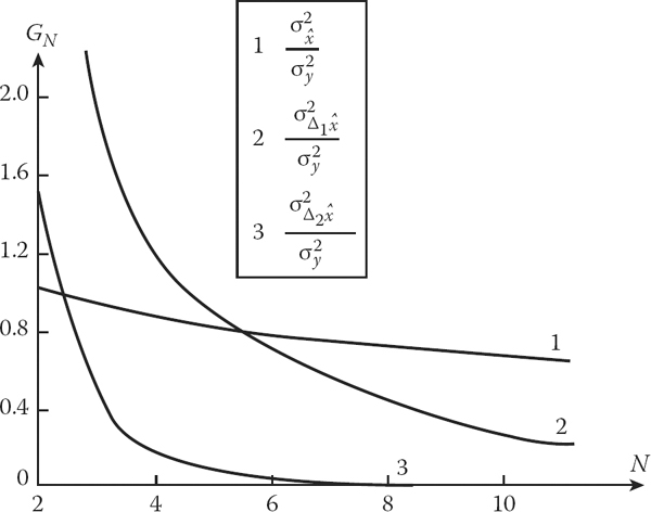
FIGURE 5.4 Coefficient of accuracy in determination of the normalized elements of error correlation matrix of second-order polynomial target track parameter estimation versus the number of measurements.

For example, at N = 3 we obtain

$Ψ_{3} = ‖ \begin{matrix} 1 & - \frac{3}{2} & \frac{1}{2} \\ - \frac{3}{2} & \frac{13}{2} & - 3 \\ \frac{1}{2} & - 3 & \frac{3}{2} \end{matrix} ‖ σ_{x}^{2} . (5.80)$

Coefficient of accuracy under determination of the normalized elements of error correlation matrix of the second-order polynomial target track parameter estimation versus the number of measurements is shown in Figure 5.4. Comparison of the diagonal elements of the matrix (5.80) that are characteristics of accuracy under estimation of the second-order polynomial target track coordinate and its first increment with analogous elements of the error correlation matrix of linear target track parameter estimation (see Figure 5.4) shows that at low values of N, the accuracy of linear target track parameter estimation is much higher than the accuracy of the second-order polynomial target track parameter estimation. Consequently, within the limits of small observation intervals, it is worth presenting the target track as using the first-order polynomial. In this case, the high quality of cancellation of random errors of target track parameter estimation by filtering is guaranteed. Dynamic errors arising owing to mismatching between the target moving hypotheses can be neglected as a consequence of the narrow approximated part of the target track.

5.4.4 ALGORITHM OF EXTRAPOLATION OF TARGET TRACK PARAMETERS

${\hat{x}}_{e x} = {\hat{x}}_{N} + {\hat{\dot{x}}}_{N} τ_{ex} + \hat{\ddot{x}} \frac{τ_{ex}^{2}}{2} + \dots + {\hat{x}}_{N}^{(s)} \frac{τ_{ex}^{(s)}}{s!}, (5.81)$

${\hat{\dot{x}}}_{e x} = {\hat{\dot{x}}}_{N} + {\hat{\ddot{x}}}_{N} τ_{ex} + \hat{\ddot{x}} \frac{τ_{ex}^{2}}{2} + \dots + {\hat{x}}_{N}^{(s)} \frac{τ_{ex}^{(s - 1)}}{(s - 1)!}, (5.82)$

${\hat{x}}_{e x}^{(s)} = {\hat{x}}_{N}^{(s)}, (5.83)$

where τ_ex = t_ex − t_N is the interval of extrapolation time. Equations 5.81 through 5.83 allow us to define the extrapolated coordinates for each specific case of target track representation. For example, in the case of linear target track at equally discrete coordinate measurement we obtain the following:

${\hat{x}}_{N + p} = \hat{x} + {\hat{\dot{x}}}_{N} + \frac{τ_{ex}}{T_{0}} T_{eq} = {\hat{x}}_{N} + Δ_{1} {\hat{x}}_{N} \frac{τ_{ex}}{T_{0}}, (5.84)$

$Δ_{1} {\hat{x}}_{N + p} = Δ_{1} {\hat{x}}_{N} . (5.85)$

Substituting in (5.84) and (5.85) the corresponding formulas for smoothed parameters, we obtain

$x_{N + p} = \frac{1}{G_{N}} [(h_{N} + \frac{τ_{e x}}{T_{0}} g_{N}) {\sum^{}}_{i = 1}^{N} w_{i} x_{i} - (g_{N} + \frac{τ_{e x}}{T_{0}} f_{N}) \sum_{i = 1}^{N} w_{i} (N - i) x_{i}] . (5.86)$

If, additionally, these measurements are uniformly precise, we obtain

${\hat{x}}_{N + p} = \sum_{i = 1}^{N} [η_{\hat{x}} (i) + \frac{τ_{e x}}{T_{e q}} η_{Δ_{1} \hat{x}} (i)] x_{i} . (5.87)$

At τ_ex = T_eq, we have

${\hat{x}}_{N + 1} = \sum_{i = 1}^{N} η_{{\hat{x}}_{N + 1}} (i) x_{i}, (5.88)$

where

$η_{{\hat{x}}_{N + 1}} (i) = \frac{2 (3 - N - 2)}{N (N - 1)} (5.89)$

is the weight function of measured coordinate magnitudes under the target track parameter extrapolation per one measurement period.

The error correlation matrix of linear target track parameter extrapolation takes the following form at equally discrete coordinate measurement:

$Ψ_{N + p} = \frac{1}{G_{N}} ‖ \begin{array}{l} h_{N} + 2 \frac{τ_{e x}}{T_{0}} g_{N} + {(\frac{τ_{e x}}{T_{0}})}^{2} & g_{N} + \frac{τ_{e x}}{T_{0}} f_{N} \\ g_{N} + \frac{τ_{e x}}{T_{0}} f_{N} & f_{N} \end{array} ‖ . (5.90)$

If, additionally, these measurements are uniformly precise, we obtain the following elements of the error correlation matrix of linear target track parameter extrapolation:

$ψ_{11} = \frac{2 [(N - 1) (2 N - 1) + 6 (τ_{e x} / T_{e q}) (N - 1) + 6 {(τ_{e x} / T_{e q})}^{2}]}{N (N^{2} - 1)} σ_{x}^{2}; (5.91)$

$ψ_{12} = ψ_{21} = \frac{6 [(N - 1) + (τ_{e x} / T_{e q})]}{N (N^{2} - 1)} σ_{x}^{2}; (5.92)$

$ψ_{22} = \frac{12}{N (N^{2} - 1)} σ_{x}^{2} . (5.93)$

If the independent target track parameter coordinate is represented by the polynomial of the second order, the target track parameter extrapolation formulas and the error correlation matrix of linear target track parameter extrapolation are obtained in an analogous way.

5.4.5 DYNAMIC ERRORS OF TARGET TRACK PARAMETER ESTIMATION USING POLAR COORDINATE SYSTEM

Sometimes we use the polynomial deterministic model of target track parameter estimation to represent changes in polar coordinate r_tg and β_tg of the target track. The polynomial representation of polar coordinates does not reflect the true law of target moving and allows us only to approximate with the previously given accuracy the target movement law within the limits of finite observation interval. In the case of a uniform and straight-line target moving with arbitrary course at the fixed altitude with respect to the stationary radar system, the law of changing the polar coordinates (see Figure 5.5) is determined by the following form:

$r_{t g} (t) = \sqrt{r_{0}^{2} + {[V_{t g} (t - t_{0})]}^{2}}; (5.94)$

$β_{t g} (t) = β_{0} + \arctan [\frac{V_{t g} (t - t_{0})}{r_{0}}], (5.95)$

Images

FIGURE 5.5 Target moving in polar coordinates.

where

r₀ and β₀ are the range and azimuth of the nearest to origin point on the target track (the point A on Figure 5.5)
t₀ is the time of target flight to the point A
V_tg is the target velocity. In the case of a target moving on circular arc within the limits of maneuver segment or mutual target moving and replacement of the CRS, we obtain the formulas that are analogous to (5.94) and (5.95) by structure but complex by essence

As follows from (5.94) and (5.95), even in the simplest cases of linear target movement and a stationary CRS, the polar coordinates are changed according to nonlinear laws. This nonlinearity becomes intensified as it is passed to complex target moving models, especially under the moving CRS. Inconsistency between the polynomial model and nonlinear character in changing the vector of estimated target track parameters leads to dynamical errors in smoothing, which can be presented in the form of differences between the true value of the vector of estimated target track parameters and the mathematical expectation of estimate of this vector, namely,

$Δ θ_{g} = [θ - E (\hat{θ})] . (5.96)$

To describe the dynamical errors of estimations of the target track parameters by algorithms that are synthesized by the maximum likelihood criterion and using the target track polynomial model, we employ the well-known theory of errors in the approximation of arbitrary continuously differentiable function f(t) within the limits of the interval t_N − t₀ by the polynomial function of the first or second order using the technique of least squares. This function takes the following form:

${\begin{matrix} \begin{array}{l} ℱ_{1} (t) = a_{0} + a_{1} (t - t_{0}), \\ ℱ_{2} (t) = a_{0} + a_{1} (t - t_{0}) + 0.5 a_{2} {(t - t_{0})}^{2} . \end{array} \end{matrix} (5.97)$

In the case of linear target track, the coefficients a₀ and a₁ are defined from the following system of equations:

${\begin{array}{l} \int_{t_{0}}^{t_{N}} [f (t) - a_{0} - a_{1} (t - t_{0})] d t = 0, \\ \int_{t_{0}}^{t_{N}} [f (t) - a_{0} - a_{1} (t - t_{0})] t d t = 0. \end{array} (5.21)$

Solution of the equation system (5.98) is found under expansion of the function f(t) by Taylor series at the point 0.5(t_N + t₀), that is, in the middle of the approximation interval, namely,

$f (t) = f [0.5 (t_{0} + t_{N})] + \sum_{k = 1}^{\infty} \frac{b_{k}}{k!} {[t - 0.5 (t_{0} + t_{N})]}^{k}; (5.99)$

$b_{k} = {\frac{d^{k} [f (t)]}{d t^{k}} |}_{t = 0.5 (t_{0} + t_{N})} . (5.100)$

The error of approximation at the point t = t_N can be determined in the following form:

$Δ f (t_{N}) = f (t_{N}) - ℱ_{1} (t_{N}) . (5.101)$

Investigations and computations made by this procedure give us the following results. Under linear approximation of polar coordinates, the maximum dynamic errors take the following form:

${\begin{array}{l} Δ r_{d}^{\max} \approx \frac{{(N - 1)}^{2} T_{e q}^{2} V_{t g}^{2}}{12 r_{\min}}, \\ Δ β_{d}^{\max} \approx \frac{\sqrt{3} {(N - 1)}^{2} T_{e q}^{2} V_{t g}^{2}}{32 r_{\min}^{2}}; \end{array} (5.102)$

${\begin{array}{l} Δ r_{d}^{\max} \approx \frac{(N - 1) T_{eq} V_{tg}^{2}}{2 r_{\min}}, \\ Δ {\dot{β}}_{d}^{\max} \approx \frac{3 \sqrt{3} (N - 1) T_{eq} V_{tg}^{2}}{16 r_{\min}^{2}}; \end{array} (5.103)$

where N is the number of coordinate readings within the limits of the observation interval t_N − t₀. In the case of quadratic approximation of the polar coordinates, the formulas for the maximum dynamic errors are more complex and we omit them.

Comparison of the dynamic errors of approximation of the polar coordinates by the polynomials of the first and second power at the same values of the target track parameters V_tg, r_min, and T_eq and the sample size (N − 1)T_eq shows that the dynamic errors under linear approximation are approximately one order higher than those under quadratic approximation. Moreover, under approximation of r_tg(t) and β_tg(t) by the polynomials of the second power, the dynamical errors are small in comparison with random errors and we can neglect them. However, as shown by simulation, if the target is in an in-flight maneuver and the CRS is moving, the dynamical errors increase essentially, because nonlinearity in changing the polar coordinates increases sharply at the same time.

5.5 Recurrent Filtering Algorithms of Undistorted Polynomial Target Track Parameters

5.5.1 OPTIMAL FILTERING ALGORITHM FORMULA FLOWCHART

Methods of estimation of the target track parameters based on the fixed sample of measured coordinates, which are discussed in the previous sections, are used, as a rule, at the beginning of the detected target trajectory. Implementation of these methods in the course of tracking is not worthwhile owing to the complexity and insufficient accuracy defined by the small magnitude of employed measures. Accordingly, there is a need to employ the recurrent algorithms ensuring a sequential, that is, after each new coordinating measurement, adjustment of target track parameters and their filtering purposes. At the recurrent filter output, we obtain the target track parameter estimations caused by the last observation. For this reason, a process of recurrent evaluation is called further the sequential filtering, and corresponding algorithms are called the algorithms of sequential filtering of target track parameters.

In a general case, the problem of synthesis of the sequential filtering algorithm for a set or vector of target track parameters is defined in the following way. Let the model of the undistorted target track be given by the following difference equation:

$θ_{n} = Φ_{n} θ_{n - 1}, (5.104)$

and the observed random sequence is given by

$Y_{n} = H_{n} θ_{n} + Δ Y_{n}, (5.105)$

where

θ_n is the (s + 1)-dimensional vector of filtered target track parameters
Y_n is the l-dimensional vector of observed coordinates
ΔY_n is the l-dimensional vector of measurement errors

The sequence of these vectors is the uncorrelated random sequence with zero mean and known correlation matrix R_n; Φ_n and H_n are the known matrices defined in Section 4.2. Further, we consider that ${\hat{θ}}_{n - 1}$ is the vector of estimations of target track parameters determined by (n − 1) coordinating measurements; Ψ_n−1 is the corresponding correlation matrix of estimation errors. There is a need to obtain the formulas for ${\hat{θ}}_{n}$ , using for this purpose the vector θ_n−1 of previous estimations and results of new measurement Y_n, and also the formula for the error correlation matrix Ψ_n based on the known matrices Ψ_n−1 and R_n.

In accordance with a general estimation theory, the optimal solution of the sequential filtering problem is reduced, first of all, to a definition of the a posteriori pdf of the filtered target track parameters, because this pdf possesses all information obtained from a priori sources and observation results. Differentiating the a posteriori pdf, we can obtain the optimal estimation of target track parameters, which are interesting for us, by the maximum a posteriori probability criterion. Henceforth, we consider the optimal sequential filtering, namely, in this sense.

Thus, let the estimation vector ${\hat{θ}}_{n - 1}$ of the target track parameter vector θ_n obtained by observations of the previous (n − 1) coordinating measurement be given. We assume that pdf of the vector ${\hat{θ}}_{n - 1}$ is the normal Gaussian with the mathematical expectation θ_n−1 and correlation matrix Ψ_n−1. The vector ${\hat{θ}}_{n - 1}$ is extrapolated during the next nth measurement in accordance with the equation

${\hat{ϑ}}_{n | n - 1} = θ_{{ex}_{n}} = Φ_{n} θ_{n - 1} . (5.106)$

The specific form of the extrapolation matrix Φ_n is defined by the target track model. For example, in the case of the only coordinate x_n that can be presented by the polynomial of the second order

$θ_{n - 1} = {‖ \begin{matrix} {\hat{x}}_{n - 1} & {\hat{\dot{x}}}_{n - 1} & {\hat{\ddot{x}}}_{n - 1} \end{matrix} ‖}^{T}, (5.107)$

we have

$Φ_{n} = ‖ \begin{matrix} 1 & τ_{ex} & 0.5 τ_{ex}^{2} \\ 0 & 1 & τ_{ex} \\ 0 & 0 & 1 \end{matrix} ‖ (5.108)$

and (5.107) can be presented in the following form:

${\hat{θ}}_{{ex}_{n}} = ‖ \begin{matrix} {\hat{x}}_{{ex}_{n}} \\ {\hat{\dot{x}}}_{{ex}_{n}} \\ {\hat{\ddot{x}}}_{{ex}_{n}} \end{matrix} ‖ = ‖ \begin{matrix} 1 & τ_{ex} & 0.5 τ_{ex}^{2} \\ 0 & 1 & τ_{ex} \\ 0 & 0 & 1 \end{matrix} ‖ ‖ \begin{matrix} {\hat{x}}_{n - 1} \\ {\hat{\dot{x}}}_{n - 1} \\ {\hat{\ddot{x}}}_{n - 1} \end{matrix} ‖, (5.109)$

where η_ex = t_n − t_n−1. The correlation matrix Ψ_n−1 is also extrapolated at the instant t_n by the following formula:

$Ψ_{n | n - 1} = Ψ_{{ex}_{n}} = Φ_{n} Ψ_{n - 1} Φ_{n}^{T} . (5.110)$

Taking into consideration a linearity property of the extrapolation operator Φ_n, the pdf of the vector of extrapolated target track parameters will also be normal Gaussian:

$p ({\hat{θ}}_{e x_{n}}) = C_{1} \exp [- 0.5 {({\hat{θ}}_{e x_{n}} - θ_{n})}^{T} Ψ_{e x_{n}}^{- 1} ({\hat{θ}}_{e x_{n}} - θ_{n})], (5.111)$

where

θ_n is the vector of true values of target track parameters at the instant t_n
C is the normalizing factor

The pdf given by (5.111) is the a priori pdf of the vector of estimated target track parameters before the next nth measurement. At the instant t_n, the regular measurement of target coordinates is carried out. In a general case of a 3-D CRS we obtain

$Y_{n} = {‖ \begin{matrix} r_{n} & β_{n} & ε_{n} \end{matrix} ‖}^{T} . (5.112)$

It is assumed that the errors under coordinating measurements are subjected to the normal Gaussian distribution and uncorrelated between each other for neighbor radar antenna scanning. Consequently,

$p (Y_{n} | θ_{n}) = C_{2} \exp [- 0.5 {(Y_{n} - H_{n} θ_{n})}^{T} R_{n}^{- 1} (Y_{n} - H_{n} θ_{n})], (5.113)$

where $R_{n}^{- 1}$ is the inverse correlation matrix of measure errors.

Under the assumption that there is no correlation between the measurement errors in the case of the neighbor radar antenna scanning, the a posteriori pdf for the target track parameter θ_n after n measurements is defined using the Bayes formula

$p ({\hat{θ}}_{n} | Y_{n}) = C_{3} p ({\hat{θ}}_{{ex}_{n}}) p (Y_{n} | θ_{n}), (5.114)$

and owing to the fact that pdfs of components are the normal Gaussian, the a posteriori pdf (5.115) will also be the normal Gaussian:

$p ({\hat{θ}}_{n} | Y_{n}) = C_{4} \exp [- 0.5 {({\hat{θ}}_{n} - θ_{n})}^{T} Ψ_{n}^{- 1} ({\hat{θ}}_{n} - θ_{n})], (5.115)$

where

${\hat{θ}}_{n}$ is the vector of estimated target track parameters by n measurements
Ψ_n is the error correlation matrix of estimated target track parameters

In the case of the normal Gaussian distribution, $\max p ({\hat{θ}}_{n} | Y_{n})$ corresponds to the mathematical expectation of the vector of estimated target track parameters. Consequently, the problem of target track parameter estimation by a posteriori probability maximum is reduced, in our case, to definition of the parameters ${\hat{θ}}_{n}$ and Ψ_n in (5.115). Using (5.111) through (5.114) for pdfs included in (5.115), we obtain after the logarithmic transformations the following formula:

${({\hat{θ}}_{n} - θ_{n})}^{T} Ψ_{n}^{- 1} ({\hat{θ}}_{n} - θ_{n}) = {({\hat{θ}}_{e x_{n}} - θ_{n})}^{T} Ψ_{e x_{n}}^{- 1} ({\hat{θ}}_{e x_{n}} - θ_{n}) + {(Y_{n} - H_{n} θ_{n})}^{T} R_{n}^{- 1} (Y_{n} - H_{n} θ_{n}) + const . (5.116)$

From this equation, we can find that

${\begin{array}{l} Ψ_{n}^{- 1} = Ψ_{e x_{n}}^{- 1} + H_{n}^{T} R_{n}^{- 1} H_{n}; \\ {\hat{θ}}_{n} = {\hat{θ}}_{e x_{n}} + Ψ_{n} H_{n}^{T} R_{n}^{- 1} (Y_{n} - H_{n} {\hat{θ}}_{e x_{n}}) . \end{array} (5.117)$

Taking into consideration (5.106) and (5.110) for ${\hat{θ}}_{e x_{n}}$ and $Ψ_{{ex}_{n}}$ , the main relationships of the optimal sequential filtering algorithm can be presented in the following form:

${\begin{array}{l} {\hat{θ}}_{{ex}_{n}} = Φ_{n} {\hat{θ}}_{n - 1}; \\ Ψ_{{ex}_{n}} = Φ_{n} Ψ_{n - 1} Φ_{n}^{T}; \\ Ψ_{n}^{- 1} = Ψ_{{ex}_{n}}^{- 1} + H_{n}^{T} R_{n}^{- 1} H_{n}; \\ G_{n} = Ψ_{n} H_{n}^{T} R_{n}^{- 1}; \\ {\hat{θ}}_{n} = {\hat{θ}}_{{ex}_{n}} + G_{n} (Y_{n} - H_{n} {\hat{θ}}_{{ex}_{n}}) . \end{array} (5.118)$

The system of equation (5.118) represents the optimal recurrent linear filtering algorithm and is called the Kalman filtering equations [9–16]. These equations can be transformed into a more convenient form for realization:

${\begin{array}{l} {\hat{θ}}_{{ex}_{n}} = Φ_{n} {\hat{θ}}_{n - 1}; \\ Ψ_{{ex}_{n}} = Φ_{n} Ψ_{n - 1} Φ_{n}^{T}; \\ G_{n} = Ψ_{{ex}_{n}} H_{n}^{T} {(H_{n} Ψ_{{ex}_{n}} H_{n}^{T} + R_{n})}^{- 1}; \\ {\hat{θ}}_{n} = {\hat{θ}}_{{ex}_{n}} + G_{n} (Y_{n} - H_{n} {\hat{θ}}_{{ex}_{n}}); \\ Ψ_{n} = Ψ_{{ex}_{n}} - G_{n} H_{n} Ψ_{{ex}_{n}} . \end{array} (5.119)$

A general filter flowchart realizing (5.119) is shown in Figure 5.6. A discrete optimal recurrent filter possesses the following properties:

Filtering equations have recurrence relations and can be realized well by a computer system.
Filtering equations represent simultaneously a description of procedure to realize this filter; in doing so, a part of the filter is similar to the model of target track (compare Figures 5.2 and 5.6).
The correlation matrix of errors of target track parameter estimation Ψ_n is computed independently of measuring Y_n; consequently, if statistical characteristics of measuring errors are given, then the correlation matrix Ψ_n can be computed in advance and stored in a memory device; this essentially reduces the time of realization of target track parameter filtering.

Images

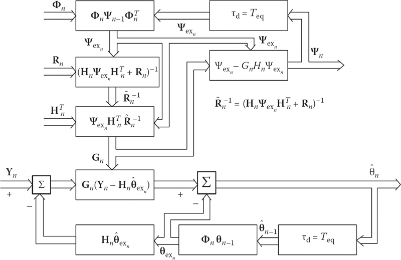
FIGURE 5.6 General Kalman filter flowchart.

5.5.2 FILTERING OF LINEAR TARGET TRACK PARAMETERS

Formulas of the sequential filtering algorithm of linear target track parameters are obtained directly from (5.119). The target track coordinate and velocity of its changes at the instant of last nth measuring are considered as the filtered parameters. We assume that all measurements are equally discrete with the period T_eq.

Assume the vector of filtered target track parameters

${\hat{θ}}_{n - 1} = ‖ \begin{matrix} {\hat{x}}_{n - 1} \\ {\hat{\dot{x}}}_{n - 1} \end{matrix} ‖ (5.120)$

and the error correlation matrix of target track parameter estimations

$Ψ_{n - 1} = \frac{1}{γ_{n - 1}} ‖ \begin{matrix} h_{n - 1} & \frac{g_{n - 1}}{T_{eq}} \\ \frac{g_{n - 1}}{T_{eq}} & \frac{f_{n - 1}}{T_{eq}^{2}} \end{matrix} ‖ (5.121)$

are obtained by the (n − 1) previous measurements of the coordinate x.
In accordance with the adopted target track model, an extrapolation of the target track coordinates at the instant of next measuring is carried out by the formula

${\hat{θ}}_{{ex}_{n}} = ‖ \begin{matrix} {\hat{x}}_{{ex}_{n}} \\ {\hat{\dot{x}}}_{{ex}_{n}} \end{matrix} ‖ = ‖ \begin{matrix} {\hat{x}}_{n - 1} + {\hat{\dot{x}}}_{n - 1} T_{eq} \\ {\hat{\dot{x}}}_{n - 1} \end{matrix} ‖ . (5.122)$
The correlation matrix of extrapolation errors is computed by the following formula:

$Ψ_{e x_{n}} = Φ_{n} Ψ_{n - 1} Φ_{n}^{T} . (5.123)$

The final version after elementary mathematical transformations takes the following form:

$Ψ_{e x_{n}} = \frac{1}{γ_{n - 1}} ‖ \begin{matrix} h_{n - 1} + 2 g_{n - 1} + f_{n - 1} & \frac{g_{n - 1} + f_{n - 1}}{T_{eq}} \\ \frac{g_{n - 1} + f_{n - 1}}{T_{eq}} & \frac{f_{n - 1}}{T_{eq}^{2}} \end{matrix} ‖ . (5.124)$
After nth measuring of the coordinate x with the variance of measuring error $σ_{x_{m}}^{2}$ , we can compute the error correlation matrix of target track parameter filtering:

$Ψ_{n} = \frac{1}{γ_{n}} ‖ \begin{matrix} h_{n} & \frac{g_{n}}{T_{eq}} \\ \frac{g_{n}}{T_{eq}} & \frac{f_{n}}{T_{eq}^{2}} \end{matrix} ‖, (5.125)$

where

${\begin{array}{l} h_{n} = h_{n - 1} + 2 g_{n - 1} + f_{n - 1}; \\ g_{n} = g_{n - 1} + f_{n}; \\ f_{n} = f_{n - 1} + v_{n}; \\ γ_{n} = γ_{n - 1} + v_{n} h_{n}; \end{array} (5.126)$

and $v_{n} = σ_{x_{m}}^{- 2}$ is the weight of the last measuring. Formulas in (5.126) allow us to form the elements of the matrix Ψ_n directly from the elements of the matrix Ψ_n−1 taking into consideration the weight of the last measuring.
The matrix coefficient of filter amplification defined as

$G_{n} = Ψ_{n} H_{n}^{T} R_{n}^{- 1} (5.127)$

in the considered case takes the following form:

$G_{n} = ‖ \begin{matrix} A_{n} \\ \frac{B_{n}}{T_{eq}} \end{matrix} ‖, (5.128)$

where

${\begin{matrix} A_{n} = \frac{h_{n} v_{n}}{γ_{n}}; \\ B_{n} = \frac{g_{n} v_{n}}{γ_{n}} . \end{matrix} (5.129)$
Taking into consideration the relations obtained, we are able to compute the estimations of linear target track parameters in the following form:

${\hat{x}}_{n} = {\hat{x}}_{e x_{n}} + A_{n} (x_{n_{m}} - {\hat{x}}_{e x_{n}}), (5.130)$

${\hat{\dot{x}}}_{n} = {\hat{\dot{x}}}_{n - 1} + \frac{B_{n}}{T_{e q}} (x_{n_{m}} - {\hat{x}}_{e x_{n}}) . (5.131)$
Under equally discrete and uniformly precise measurements of the target track coordinates, we obtain

${\begin{array}{l} f_{n} = n v; \\ g_{n} = \frac{n (n - 1)}{2} v; \\ h_{n} = \frac{n (n - 1) (2 n - 1)}{6} v; \\ γ_{n} = \frac{n^{2} (n^{2} - 1)}{12} v^{2} . \end{array} (5.132)$

Substituting (5.132) into (5.128) and (5.129), we obtain finally

${\begin{matrix} A_{n} = \frac{2 (2 n - 1)}{n (n + 1)}; \\ B_{n} = \frac{6}{n (n + 1)} . \end{matrix} (5.133)$

Dependences of the coefficients A_n and B_n versus the number of observations n are presented in Figure 5.7. As we can see from Figure 5.7, with an increase in n the filter gains on the coordinate and velocity are approximated asymptotically to zero. Consequently, with an increase in n the results of last measurements at filtering the coordinate and velocity are taken into consideration with the less weight, and the filtering algorithm ceases to respond to changes in the input signal. Moreover, essential problems in the realization of the filter arise in computer systems with limited capacity of number representation. At high n, the computational errors are accumulated and are commensurable with a value of the lower order of the computer system, which leads to losses in conditionality and positive determinacy of the correlation matrices of extrapolation errors and filtering of the target track parameters. The “filter divergence” phenomenon appears when the filtering errors increase sharply and the filter stops operating. Thus, if we do not take specific measures in correction, the optimal linear recurrent filter cannot be employed in complex automatic radar systems. Overcoming this problem is a great advance in automation of CRSs.

Images

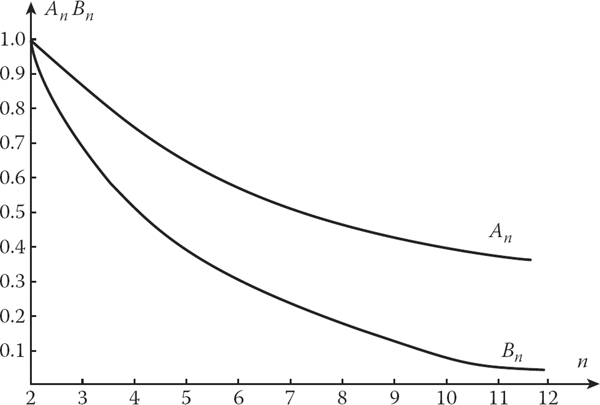
FIGURE 5.7 Coefficients A_n and B_n versus the number of observations n.

5.5.3 STABILIZATION METHODS FOR LINEAR RECURRENT FILTERS

${R^{'}}_{n} = R_{n} + α I . (5.134)$

In doing so, the regularization parameter α must satisfy the following condition:

$\frac{δ}{ε (δ)} \leq α \leq α_{0} (δ), (5.135)$

where

δ is the accuracy of matrix R_n assignment
ε(δ) and α₀(δ) are the arbitrary decreasing functions tending to approach zero as δ → 0

Thus, in the given case, a general approach to obtain the stable solutions by the regularization or smoothing method is the artificial rough rounding of measuring results. However, the employment of this method in a pure form is impossible since a way to choose the regularization parameter α is generally unknown. In practice, a cancellation of divergence of the recurrent filter can be ensured by effective limitation of memory device capacity including in the recurrent filter. Consider various ways to limit a memory device capacity in the recurrent filter.

5.5.3.1 Introduction of Additional Term into Correlation Matrix of Extrapolation Errors

In this case, we obtain

${Ψ^{'}}_{{ex}_{n}} = Φ_{n} (Ψ_{n - 1} + Ψ_{0}) Φ_{n}^{T}, (5.136)$

where Ψ₀ is the arbitrary positive definite matrix. Under separate filtering of the polynomial target track parameters using the results of equally discrete and uniformly precise coordinating measurements, we obtain

$Ψ_{0} = ‖ \begin{array}{l} c_{0} & 0 & \dots & 0 \\ 0 & c_{1} & \dots & 0 \\ \dots & \dots & \dots & \dots \\ 0 & 0 & \dots & c_{s} \end{array} ‖ σ_{x_{m}}^{2}, (5.137)$

where

$σ_{x_{m}}^{2}$ is the variance of coordinating measuring errors
c_i is the constant coefficients, i = 0,…, s

In order for the recurrent filter to have a limited memory capacity, there is a need that the components of the vector G_n should be converged to the constant values 0 < γ₀ < 1,…,0 < γ_s < 1 and be in the safe operating area of the recurrent filter.

Using filtering equations, we are able to establish a relation for each specific case between the gains γ_1n,…, γ_sn and the values c₀, c₁,…,c_s. Passing to limit as n → ∞, we are able to obtain a function between the steady-state values of the recurrent filter gain $γ_{0} = \lim_{n \to \infty} γ_{0 n}, \dots, γ_{s} = \lim_{n \to \infty} γ_{s n}$ and the values c₀, c₁,…, c_s. In the case of linear target track [18], we have

$\begin{array}{l} c_{0} = \frac{12}{(n_{ef}^{2} - 1)}; \\ c_{1} = \frac{144}{(n_{ef}^{2} - 1) (n_{ef}^{2} - 4)}, \end{array} (5.138)$

where n_ef is the fixed effective finite memory capacity of the recurrent filter. At the same time, the variances of random errors of target track parameter estimations in steady filtering coincide with analogous parameters for nonrecursive filters, namely,

$σ_{\hat{x}}^{2} = \frac{2 (2 n_{ef} - 1)}{n_{ef} (n_{ef} + 1)} σ_{x_{m}}^{2}; (5.139)$

$σ_{\hat{\dot{x}}}^{2} = \frac{12 σ_{x_{m}}^{2}}{T_{eq}^{2} n_{ef} (n_{ef} - 1)} . (5.140)$

Thus, the recurrent filter with additional term introduced into the error correlation matrix of extrapolation approximates the filter with finite memory capacity at the corresponding choice of the coefficients c₀, c₁,…, c_s.

5.5.3.2 Introduction of Artificial Aging of Measuring Errors

This operation is equivalent to a replacement of the correlation matrix R_n-i of measuring errors at the instant t_n-i by the matrix

$\begin{matrix} R_{n - 1}^{*} = \exp [c (t_{n} - t_{n - i})] R_{n - i}, & c > 0. \end{matrix} (5.141)$

Under equally discrete measurements, we have

${\begin{array}{l} t_{n} - t_{n - i} = i T_{0}; \\ \exp [c (t_{n} - t_{n - i})] = \exp [c i T_{0}] = s^{i}, \end{array} (5.142)$

where s = exp(cT₀) > 1. At the same time, the correlation matrix of extrapolation errors is determined in the following form:

${Ψ^{'}}_{{ex}_{n}} = Φ_{n} [s Ψ_{n - 1}] Φ_{n}^{T,} (5.143)$

In this case, under the equally discrete and uniformly precise coordinating measurements, the smoothing filter coefficients are converged to positive constants in the filter safe operating area. However, it is impossible to find the parameter s for this filter so that the variance and dynamic errors of these filters and the filter with finite memory capacity are matched.

5.5.3.3 Gain Lower Bound

In the simplest case of the equally discrete and uniformly precise coordinating measurements, the gain bound is defined directly by the formulas for G_n at the given effective memory capacity of the filter. Computation and simulation show that the last procedure is the best way by the criterion of realization cost and rate to define the variances of errors under the equally discrete and uniformly precise coordinating measurements from the considered procedures to limit the recurrent filter memory capacity. The first procedure, that is, the introduction of an additional term into the correlation matrix of extrapolation errors, is a little worse. The second procedure, that is, an introduction of the multiplicative term into the correlation matrix of extrapolation errors, is worse in comparison with the first and third ones by realization costs and rate of convergence of the error variance to the constant magnitude.

5.6 Adaptive Filtering Algorithms of Maneuvering Target Track Parameters

5.6.1 PRINCIPLES OF DESIGNING THE FILTERING ALGORITHMS OF MANEUVERING TARGET TRACK PARAMETERS

Until now, in considering filtering methods and algorithms of target track parameters we assume that a model equation of target track corresponds to the true target moving. In practice, this correspondence is absent, as a rule, owing to target maneuvering. One of the requirements of successful solution of problems concerning the real target track parameter filtering is to take into consideration a possible target maneuver.

The state equation of maneuvering target takes the following form:

$θ_{n} = Φ_{n} θ_{n - 1} + Γ_{n} g_{m_{n}} + K_{n} η_{n}, (5.144)$

where

Φ_nθ_n−1 is the equation of undisturbed target track, that is, the polynomial of the first order
$g_{m_{n}}$ is the l-dimensional vector of the disturbed target track parameters caused by the willful target maneuver
η_n is the p-dimensional vector of disturbances caused by stimulus of environment and uncertainty in control (control noise)
Γ_n and K_n are the known matrices

According to precision of CRS characteristics and estimated target maneuver, three approaches are possible to design the filtering algorithm of real target track parameters.

5.6.1.1 First Approach

We assume that the target has limited possibilities for maneuver; for example, there are only random unpremeditated disturbances in the target track. In this case, the second term in (5.145) is equal to zero and sampled values of the vector η_n are the sequence subjected to the normal Gaussian distribution with zero mean and the correlation matrix:

$Ψ_{η} = ‖ \begin{matrix} σ_{η r}^{2} & 0 & 0 \\ 0 & σ_{η β}^{2} & 0 \\ 0 & 0 & σ_{η ε}^{2} \end{matrix} ‖ . (5.145)$

Nonzero elements of this matrix represent a set of a priori data about an intensity of target maneuver by each coordinate (r, β, ε). In this case, a record of target track disturbance in the filtering algorithm is reduced to filter bandwidth increase. For this purpose, a computation of the error correlation matrix of target track parameter estimations into an extrapolated point is carried out by the formula

$Ψ_{{ex}_{n}} = Φ_{n} Ψ_{n - 1} Φ_{n}^{T} + K_{n} Ψ_{η} K_{n}^{T}, (5.146)$

where the s × l matrix K_n can be presented in the following form:

$K_{n} = ‖ \begin{array}{l} 0.5 τ_{{ex}_{n}}^{2} & 0 & 0 \\ τ_{{ex}_{n}} & 0 & 0 \\ 0 & 0.5 τ_{{ex}_{n}}^{2} & 0 \\ 0 & τ_{{ex}_{n}} & 0 \\ 0 & 0 & 0.5 τ_{{ex}_{n}}^{2} \\ 0 & 0 & τ_{{ex}_{n}} \end{array} ‖, (5.147)$

$τ_{{ex}_{n}} = t_{n} - t_{n - 1}$ is the interval of target track parameter extrapolation. Other formulas of the recurrent filtering algorithm are the same as in the case of a nonmaneuvering target.

There is a need to note that the methods discussed in the previous section to limit the memory capacity of the recurrent filter by their sense and consequences are equivalent to the considered method to record the target maneuver since a limitation in memory capacity of the recurrent filter, increasing a stability, can simultaneously decrease the sensitivity of the filter to short target maneuvering.

5.6.1.2 Second Approach

We assume that the target performs only a single premeditated maneuver of high intensity within the observation time interval. In this case, the target track can be divided into three parts: before the start of, in the course of, and after finishing the target maneuver. In accordance with this target track division, the intensity vector of a premeditated target maneuver can be presented in the following form:

$g_{m} (t_{i}) = {\begin{array}{l} 0 & at & t_{i} < t_{start}; \\ g_{m_{i}} & at & t_{start} \leq t_{i} \leq t_{finish}; \\ 0 & at & t_{i} > t_{finish}; \end{array} (5.148)$

where t_start and t_finish are the instants to start and finish the target maneuver. In this case, the intensity vector of target maneuver as well as the instants to start and finish the target maneuvering are subjected to statistical estimation by totality of input signals (measuring coordinates). Consequently, in the given case, the filtering problem is reduced to designing a switching filtering algorithm or switching filter with switching control based on the analysis of input signals. This algorithm concerns the class of simplest adaptive algorithms with a self-training system.

5.6.1.3 Third Approach

It is assumed that the targets subjected to tracking have good maneuvering abilities and are able to perform a set of maneuvers within the limits of observation time. These maneuvers are related to air miss relative to other targets or flight in the space given earlier. In this case, to design the formula flowchart of filtering algorithms of target track parameters, there is a need to have data about the mathematical expectation $E (g_{m_{n}})$ and the variance $σ_{g}^{2}$ of target maneuver intensity for each target and within the limits of each interval of information updating. These data (estimations) can be obtained only based on an input information analysis, and the filtering is realized by the adaptive recurrent filter.

Henceforth, we consider the principles of designing the adaptive recurrent filter based on the Bayes approach to define the target maneuver probability [19].

5.6.2 IMPLEMENTATION OF MIXED COORDINATE SYSTEMS UNDER ADAPTIVE FILTERING

To solve the problem of target maneuver detection and based on other considerations, it is worthwhile to carry out filtering of the target track parameters using the Cartesian coordinate system, the origin of which is matched with the CRS location. This coordinate system is called the local Cartesian coordinate system. The formulas of coordinate transformation from the spherical coordinate system to the local Cartesian one are given by (see Figure 5.8)

${\begin{array}{l} x = r \cos ε cos β; \\ y = r \cos ε sin β; \\ z = r \sin ε . \end{array} (5.149)$

Images

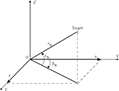
FIGURE 5.8 Transformation from the spherical coordinate system into the local Cartesian coordinate system.

Transformation to the local Cartesian coordinate system leads to an appearance of nonuniform precision and correlation between the coordinates at the filter input, which in turn leads to complexity of filter structure and additional computer cost in realization. Also, there is a need to take into consideration that other operations of signal reprocessing by a CRS, for example, target pip gating, target pip identification and so on, are realized in the simplest form in the spherical coordinate system. For this reason, the filtered target track parameters must be transformed from the local Cartesian coordinate system to the spherical one during each step of target information update.

Thus, to solve the problem of adaptive filtering of the track parameters of maneuvering targets, it is worthwhile to employ the recurrent filters, where the filtered target track parameters are represented in the Cartesian coordinate system and comparison between the measured and extrapolated coordinates is carried out in the spherical coordinate system. In this case, a detection of target maneuver or definition of the probability performance of target maneuver can be organized based on the analysis of deviation of the target track parameter estimations from magnitudes corresponding to the hypotheses of straight-line and uniform target moving.

Consider the main relationships of the recurrent filter, in which the filtered target track parameters are represented in the local Cartesian coordinate system and a comparison between the extrapolated and measured target track parameters coordinates is carried out in the spherical coordinate system. Naturally, the linear filter is considered as the basic filter, and equations defining the operation abilities of the considered linear filter are represented by the equation system given by (5.119). For simplicity, we can be restricted by the case of a two-dimensional radar measured CRS that defines the target range r_tg and azimuth β_tg. In this case, the transposed vector of target track moving parameters at the previous (n − 1) step takes the following form:

$θ_{n - 1}^{T} = ‖ \begin{matrix} {\hat{x}}_{n - 1} & {\hat{\dot{x}}}_{n - 1} & {\hat{y}}_{n - 1} & {\hat{\dot{y}}}_{n - 1} \end{matrix} ‖, (5.150)$

and the error correlation matrix of the target track parameter estimations contains 4 × 4 nonzero elements:

$Ψ_{n - 1} = ‖ \begin{matrix} Ψ_{11 (n - 1)} & Ψ_{12 (n - 1)} & Ψ_{13 (n - 1)} & Ψ_{14 (n - 1)} \\ Ψ_{21 (n - 1)} & Ψ_{22 (n - 1)} & Ψ_{23 (n - 1)} & Ψ_{24 (n - 1)} \\ Ψ_{31 (n - 1)} & Ψ_{32 (n - 1)} & Ψ_{33 (n - 1)} & Ψ_{34 (n - 1)} \\ Ψ_{41 (n - 1)} & Ψ_{42 (n - 1)} & Ψ_{43 (n - 1)} & Ψ_{44 (n - 1)} \end{matrix} ‖ . (5.151)$

Extrapolation of target track parameters is carried out in accordance with the hypothesis about the target straight-line movement, and the correlation matrix is extrapolated by the following rule:

$Ψ_{{ex}_{n}} = Φ_{n} Ψ_{n - 1} Φ_{n}^{T}, (5.152)$

where

$Φ_{n} = Φ = ‖ \begin{array}{l} 1 & T_{0} & 0 & 0 \\ 0 & 1 & 0 & 0 \\ 0 & 0 & 1 & T_{0} \\ 0 & 0 & 0 & 1 \end{array} ‖ . (5.153)$

Extrapolated polar coordinates are determined from the Cartesian coordinates by the following formulas:

${\hat{r}}_{{ex}_{n}} = \sqrt{{\hat{x}}_{e x_{n}}^{2} + {\hat{y}}_{{ex}_{n}}^{2}}, (5.154)$

$β_{{ex}_{n}} = {\begin{array}{l} A = \arctan | \frac{{\hat{y}}_{{ex}_{n}}}{{\hat{x}}_{{ex}_{n}}} |, & {\hat{x}}_{{ex}_{n}} > 0, & {\hat{y}}_{{ex}_{n}} > 0, \\ π - A, & {\hat{x}}_{{ex}_{n}} < 0, & {\hat{y}}_{{ex}_{n}} > 0, \\ π - A, & {\hat{x}}_{{ex}_{n}} < 0, & {\hat{y}}_{{ex}_{n}} < 0, \\ 2π - A, & {\hat{x}}_{{ex}_{n}} > 0, & {\hat{y}}_{{ex}_{n}} < 0. \end{array} (5.155)$

The vector of measured target track parameter coordinates and the error correlation matrix take the following form:

$Y_{n} = ‖ \begin{matrix} r_{n} \\ β_{n} \end{matrix} ‖ (5.156)$

and

$R_{n} = ‖ \begin{matrix} σ_{r_{n}}^{2} & 0 \\ 0 & σ_{r_{n}}^{2} \end{matrix} ‖ . (5.151)$

To establish a relationship between the measured coordinates and estimated target track parameters, we use the linearized operator:

$P = {‖ \begin{array}{l} \frac{\partial r}{\partial x} & 0 & \frac{\partial r}{\partial y} & 0 \\ \frac{\partial β}{\partial x} & 0 & \frac{\partial β}{\partial y} & 0 \end{array} ‖}_{x = {\hat{x}}_{{ex}_{n}}, y = {\hat{y}}_{{ex}_{n}}} . (5.158)$

This operator can be presented in the following form:

$P = ‖ \begin{matrix} P_{r}^{T} \\ P_{β}^{T} \end{matrix} ‖, (5.159)$

where

$\begin{matrix} P_{U}^{T} = ‖ \begin{matrix} \frac{\partial U}{\partial x} & 0 & \frac{\partial U}{\partial y} & 0 \end{matrix} ‖ & and & U = {r, β} \end{matrix} . (5.160)$

Henceforward, the error correlation matrix Ψ_n of the target track parameter estimations is determined by n measurements. The matrix filter gain is determined in the following way:

$G_{n} = Ψ_{n} P^{T} R_{n}^{- 1} = Ψ_{n} ‖ \begin{matrix} P_{r} & P_{β} \end{matrix} ‖ ‖ \begin{matrix} w_{r_{n}} & 0 \\ 0 & w_{β_{n}} \end{matrix} ‖ . (5.161)$

By this reason, the vector of target track parameter estimations is determined by the following formula:

${\hat{θ}}_{n} = {\hat{θ}}_{{ex}_{n}} + Ψ_{n} ‖ \begin{matrix} P_{r} & P_{β} \end{matrix} ‖ ‖ \begin{matrix} w_{r_{n}} & 0 \\ 0 & w_{β_{n}} \end{matrix} ‖ ‖ \begin{matrix} r_{n} - {\hat{r}}_{{ex}_{n}} \\ β_{n} - {\hat{β}}_{{ex}_{n}} \end{matrix} ‖ . (5.162)$

From this formula it is easy to obtain the final expression for components of the vector θ_n. Thus, in the case of ${\hat{x}}_{n}$ we obtain

${\hat{x}}_{n} = {\hat{x}}_{e x_{n}} + α_{r} w_{r_{n}} (r_{n} - {\hat{r}}_{e x_{n}}) + α_{β} w_{β_{n}} (β_{n} - {\hat{β}}_{e x_{n}}), (5.163)$

where

$α_{r} = Ψ_{11 (n)} \frac{\partial r}{\partial x} + Ψ_{13 (n)} \frac{\partial r}{\partial y}; (5.164)$

$α_{β} = Ψ_{11 (n)} \frac{\partial β}{\partial x} + Ψ_{13 (n)} \frac{\partial β}{\partial y} . (5.165)$

Other components are determined by analogous formulas.

From the earlier discussion and the relationships obtained, it follows that there is a statistical dependence between estimations of target track parameters by all coordinates in the considered filter. This fact poses difficulties in obtaining the target track parameter estimations and leads to tightened requirements for computer subsystems of a CRS. We can decrease the computer cost by refraining from optimal filtering of target track parameters that makes the filter simple. In particular, a primitive simplification is a rejection of joint filtering of target track parameters and passage to individual filtering of Cartesian coordinates with subsequent transformation of obtained target track parameter estimation coordinates to the polar coordinate system. The procedure of simplified filtering follows.

Each pair of measured coordinates r_n and β_n is transformed to the Cartesian coordinate system before filtering using the following formulas:

$\begin{matrix} x_{n} = r_{n} \cos β_{n} & and & y_{n} = r_{n} \sin β_{n} . \end{matrix} (5.166)$

The obtained values x_n and y_n are considered as independent measured coordinates with the variances of measurement errors:

$σ_{x_{n}}^{2} = \cos^{2} β_{n} σ_{r_{n}}^{2} + r_{n}^{2} \sin^{2} β_{n} σ_{β_{n}}^{2}, (5.167)$

$σ_{y_{n}}^{2} = \sin^{2} β_{n} σ_{r_{n}}^{2} + r_{n}^{2} \cos^{2} β_{n} σ_{β_{n}}^{2} . (5.168)$
Each Cartesian coordinate is filtered independently in accordance with the adopted hypothesis of Cartesian coordinate changing. The problems of detection or definition of statistical parameters of target maneuver by each coordinate are solved simultaneously.
Extrapolated values of Cartesian coordinates are transformed into the polar coordinate system by the formulas (5.154) and (5.155).

Comparison of accuracy characteristics of optimal and simple filtering procedures with double transformation of coordinates is carried out by simulation. For example, the dependences of root-mean-square error magnitudes of target track azimuth coordinate versus the number of measurements (the target track is indicated in the right top corner) for optimal (curve 1) and simple (curve 2) filtering algorithms at r_min = 10 and 20 km are shown in Figure 5.9. From Figure 5.9, we see that in the case of a simple filter, accuracy deteriorates from 5–15% against the target range, course, speed, and the number of observers. At r_min < 10 km, this deterioration in accuracy is for about 30%. However, the computer cost is decreased approximately by one order.

Images

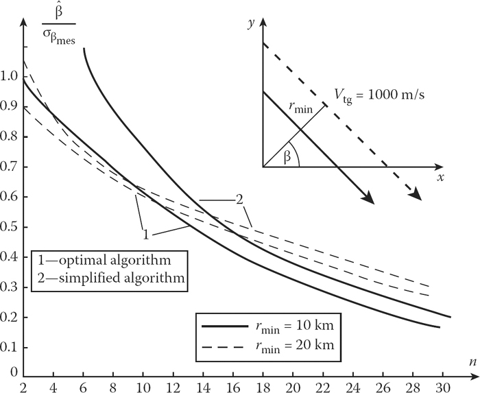
FIGURE 5.9 Root-mean-square errors of azimuth target track coordinate versus the number of measurements. Curve 1—τ_min = 10 km; curve 2—τ_min = 20 km.

5.6.3 ADAPTIVE FILTERING ALGORITHM VERSION BASED ON BAYESIAN APPROACH IN MANEUVERING TARGET

Under adaptive filtering, the linear dynamic system described by the state equation given by (5.144) is considered as the target track model. Target track distortions caused by a deliberate target maneuver are represented as a random process, the mean $E (g_{m_{n}})$ of which is changed step-wise taking a set of fixed magnitudes (states) within the limits of range $[- g_{m_{\max}}, + g_{m_{\max}}]$ . Transitions of a step-wise process from the state i to the state j are carried out with the probability P_ij ≥ 0 defined by a priori data about the target maneuver. The time when the process is in the state i before transition into the state j is the random variable with arbitrary pdf p(t_i). The mathematical model of this process is the semi-Markov random process. Distortions of the target track caused by a deliberate target maneuver and errors of intensity estimations of deliberate target maneuver are characterized by the random component η_n in an adaptive filtering algorithm. The matrices Φ_n, Γ_n, and K_n are considered as the known matrices.

Initially, we consider the Bayesian approach to design the adaptive filtering algorithm for the case of continuous distortion action $g_{m_{n}}$ . As is well known, an optimal estimation of the parametric vector θ_n at the quadratic loss can be defined from the following relationship:

${\hat{θ}}_{n} = \int_{(Θ)} θ_{n} p (θ_{n} | {Y}_{n}) d θ_{n}, (5.169)$

where

(Θ) is the space of possible values of estimated target track parameter
p(θ_n | {Y}_n) is the a posteriori pdf of the vector θ_n by data of n-dimensional sequence of measurements {Y}_n

Under the presence of the distortion parameter g_m, the a posteriori pdf of the vector θ_n can be written in the following form:

$p (θ_{n} | {Y}_{n}) = \int_{(g_{m})} p (θ_{n} | g_{m_{n}}, {Y}_{n}) p (g_{m_{n}} | {Y}_{n}) d g_{m_{n}}, (5.170)$

where (g_m) is the range of possible values of the parameter of distortions. Consequently,

${\hat{θ}}_{n} = \int_{(Θ)} θ_{n} \int_{(g_{m})} p (θ_{n} | g_{m_{n}}, {Y}_{n}) p (g_{m_{n}} | {Y}_{n}) d g_{m_{n}} d θ_{n} = \int_{(g_{m})} {\hat{θ}}_{n} (g_{m_{n}}) p ({\hat{θ}}_{n} | g_{m_{n}}, {Y}_{n}) d g_{m_{n}} . (5.171)$

Thus, the problem of estimating the vector ${\hat{θ}}_{n}$ is reduced to weight averaging the estimations ${\hat{θ}}_{n} (g_{m_{n}})$ , which are the solution of the filtering problem at the fixed magnitudes of $g_{m_{n}}$ . The estimations ${\hat{θ}}_{n} (g_{m_{n}})$ can be obtained in any way that minimizes the MMSE criterion including the recurrent linear filter or Kalman filter. The problem of optimal adaptive filtering will be solved when the a posteriori pdf $p (g_{m_{n}} | {Y}_{n})$ is determined at each step. Determination of this pdf by sample of measurements {Y}_n and its employment with the purpose of obtaining the weight estimations is the main peculiarity of the adaptive filtering method considered.

In the case considered here, when the parametric disturbance takes only the fixed magnitudes $g_{m_{j}}$ , j = −0.5m,…, −1,0,1,…,0.5m, m is even, we obtain the following formula instead of (5.171):

${\hat{θ}}_{m_{n}} = \sum_{j = - 0.5 m}^{0.5 m} θ_{n} (g_{m_{j n}}) P (g_{m_{j n}} | {Y}_{n}), (5.172)$

where $P (g_{m_{j n}} | {Y}_{n})$ is the a posteriori probability of the event $g_{m_{j n}} = g_{m_{j}}$ by data of n measurements {Y}_n. To determine the a posteriori probability $P (g_{m_{j n}} | {Y}_{n})$ , we use the Bayes rule, in accordance with which (5.17) we can write

$P (g_{m_{^{j n}}} | {Y}_{n}) = P_{n_{j}} = \frac{P (g_{m_{j n}} | {Y}_{n - 1}) p (Y_{n} | g_{m_{\dot{j}, n - 1}})}{{\sum^{}}_{j = - 0.5 m}^{0.5 m} P (g_{m_{\dot{j} n}} | {Y}_{n - 1}) p (Y_{n} | g_{m_{\dot{j}, n - 1}})} . (5.173)$

In this formula, $P (g_{m_{\dot{j} n}} | {Y}_{n - 1})$ is the a priori probability of the parameter $g_{m_{j}}$ at the nth step obtained by (n − 1) measurements and computed by the formula

$P (g_{m_{\dot{j} n}} | {Y}_{n - 1}) = \sum_{i = - 0.5 m}^{0.5 m} P_{i j} P (g_{m_{j n - 1}} | {Y}_{n - 1}), (5.174)$

where

$P_{i j} = P (g_{m_{n}} = g_{m_{j}} | g_{m_{n - 1}} = g_{m_{i}}) (5.175)$

is the conditional probability of the transition of disturbance process from the state i at the (n − 1)th step to the state j at the nth step; $p (Y_{n} | g_{m_{j, n - 1}})$ is the conditional pdf of observed magnitude of the coordinate Y_n when the parametric disturbance at the previous (n − 1)th step takes the magnitude $g_{m_{j}}$ . This pdf can be approximated by the normal Gaussian distribution with the mean determined by

$Y_{{ex}_{n, j}} = H_{n} [Φ_{n - 1} + Γ_{n - 1} g_{m_{j}}] (5.176)$

and the variance given by

$σ_{n}^{2} = H_{n} Ψ_{{ex}_{n}} H_{n}^{T} + σ_{Y_{n}}^{2} . (5.177)$

Taking into consideration (5.177) and (5.178), we obtain the a posteriori probability in the following form:

$P_{n j} = \frac{\sum_{i = - 0.5 m}^{0.5 m} P_{i j} P (g_{m_{i, n - 1}} | {Y}_{n - 1}) \exp [- {({\hat{Y}}_{n} - {\hat{Y}}_{e x_{n, \dot{j}}})}^{2} / 2 σ_{n}^{2}]}{\sum_{j = - 0.5 m}^{0.5} \sum_{i = - 0.5 m}^{0.5} P_{i j} P (g_{m_{i, n - 1}} | {Y}_{n - 1}) \exp [- {(Y_{n} - Y_{e x_{n, \dot{j}}})}^{2} / 2 σ_{n}^{2}]} . (5.178)$

The magnitudes P_nj for each j are the weight coefficients at averaging of estimations of filtered target track parameters.

Henceforth, we assume that the target track parameters are filtered individually by each Cartesian coordinate of the target. Measured values of spherical coordinates are transformed into Cartesian coordinates outside the filter. Correlation of measure errors of the Cartesian coordinates is not taken into consideration. The Cartesian coordinates fixing the intensity $g_{m_{x}}$ , $g_{m_{y}}$ , and $g_{m_{z}}$ of deliberate target maneuver are also considered as independent between each other and $g_{m_{x}} = {\ddot{x}}_{m}$ , $g_{m_{y}} = {\ddot{y}}_{m}$ , and $g_{m_{y}} = {\ddot{z}}_{m}$ . In the following, the equations of adaptive filtering algorithm applying to the Cartesian coordinate x are written in detailed form.

Step 1: Let at the (n − 1)th step be obtained ${\hat{x}}_{n - 1}$ and ${\hat{\dot{x}}}_{n - 1}$ —the estimations of target track parameters; the error correlation matrix of the target track parameter estimations takes the following form:

$Ψ_{n - 1} = ‖ \begin{matrix} ψ_{11, (n - 1)} & ψ_{12, (n - 1)} \\ ψ_{21, (n - 1)} & ψ_{22, (n - 1)} \end{matrix} ‖; (5.179)$

$P ({\ddot{\ddot{x}}}_{m_{j, n - 1}} | {x}_{n - 1})$ —the a posteriori probabilities of magnitudes of the disturbance parameter j = −0.5m,…, −1, 0, +1,…,0.5m; $σ_{{\ddot{x}}_{n - 1}}^{2}$ —the variance of random component disturbed the target track.
Step 2: Extrapolation of target track parameters for each possible magnitude of ${\ddot{x}}_{m j}$ is carried out in accordance with the following formulas:

${\begin{array}{l} {\hat{x}}_{{ex}_{n j}} = {\hat{x}}_{n - 1} + τ_{ex} {\hat{\dot{x}}}_{n - 1} + 0.5 τ_{ex}^{2} {\ddot{x}}_{m_{j}}; \\ {\hat{\dot{x}}}_{{ex}_{n j}} = {\hat{\dot{x}}}_{n - 1} + τ_{ex} {\ddot{x}}_{m_{j}} . \end{array} (5.180)$
Step 3: Elements of the error correlation matrix of extrapolation are defined by the following formulas:

${\begin{array}{l} ψ_{11_{{ex}_{n}}} = ψ_{11, n - 1} + 2 τ_{ex} ψ_{12, n - 1} + τ_{ex}^{2} ψ_{22, n - 1} + 0.25 τ_{ex}^{4} σ_{{\ddot{x}}_{n - 1}}^{2}; \\ ψ_{12_{{ex}_{n}}} = ψ_{21_{{ex}_{n}}} = ψ_{12, n - 1} + τ_{ex} ψ_{22, n - 1} + 0.5 τ_{ex}^{3} σ_{{\ddot{x}}_{n - 1}}^{2}; \\ ψ_{22, n} = ψ_{22, n - 1} + 0.5 τ_{ex}^{3} σ_{{\ddot{x}}_{n - 1}}^{2}; \end{array} (5.181)$
Step 4: Components of the filter gain vector at the nth step are defined in the following form:

${\begin{matrix} G_{1 n} = \frac{ψ_{11, e x_{n}}}{ψ_{11, e x_{n}} + σ_{x_{n}}^{2}} = ψ_{11, e x_{n}} z_{n}^{- 1} \\ G_{2 n} = \frac{ψ_{21, e x_{n}}}{ψ_{11, e x_{n}} + σ_{x_{n}}^{2}} = ψ_{21, e x_{n}} z_{n}^{- 1} \end{matrix}; (5.182)$
where

$z_{n}^{- 1} = \frac{1}{ψ_{11, e x_{n}} + σ_{x_{n}}^{2}}, (5.183)$
$σ_{x_{n}}^{2}$ is the variance of errors under measuring the coordinate x at the nth step.
Step 5: Elements of correlation matrix of errors of target track parameter estimation at the nth step are defined by the following formulas:

${\begin{array}{l} ψ_{11, n} = ψ_{11, {ex}_{n}} z_{n}^{- 1} σ_{x_{n}}^{2}; \\ ψ_{12, n} = ψ_{21, n} = ψ_{11, {ex}_{n}} σ_{x_{n}}^{2}; \\ ψ_{22, n} = ψ_{22, {ex}_{n}} = - ψ_{12}^{2}_{{,ex}_{n}} z_{n}^{- 1} . \end{array} (5.184)$
Step 6: Estimations of filtered target track parameters for each discrete value of parametric disturbance are defined in the following form:

${\begin{array}{l} {\hat{x}}_{n j} = {\hat{x}}_{{ex}_{n j}} + γ_{1 n} (x_{n} - {\hat{x}}_{{ex}_{n j}}); \\ {\hat{\dot{x}}}_{n j} = {\hat{\dot{x}}}_{{ex}_{n j}} + γ_{2 n} (x_{n} - {\hat{x}}_{{ex}_{n j}}), \end{array} (5.185)$
where x_n is the result of measuring the coordinate x at the nth step.
Step 7: The weight of discrete values of disturbance is defined as

$P ({\ddot{x}}_{m_{\dot{j} n}} | {Y}_{n}) = \frac{\sum_{i = - 0.5 m}^{0.5 m} P_{i j} P ({\ddot{x}}_{m_{i, n - 1}} | {Y}_{n - 1}) \exp [- 0.5 {(x_{n} - {\hat{x}}_{e x_{n j}})}^{2} z_{n}^{- 1}]}{\sum_{j = - 0.5 m}^{0.5 m} \sum_{i = - 0.5 m}^{0.5 m} P_{i j} P ({\ddot{x}}_{m_{i, n - 1}} | {Y}_{n - 1}) \exp [- 0.5 {(x_{n} - {\hat{x}}_{e x_{n j}})}^{2} z_{n}^{- 1}]} . (5.186)$
Step 8: The weight values of target track parameter estimations are defined as

${\begin{array}{l} {\hat{x}}_{n} = \sum_{j = - 0.5 m}^{0.5 m} {\hat{x}}_{n_{j}} P ({\ddot{x}}_{m_{j n}} | {Y}_{n}); \\ {\hat{\dot{x}}}_{n} = \sum_{j = - 0.5 m}^{0.5 m} {\hat{\dot{x}}}_{n_{j}} P ({\ddot{x}}_{m_{j n}} | {Y}_{n}) . \end{array} (5.187)$
Step 9: The weight value of discrete parametric disturbance at the nth step is defined as

${\hat{\ddot{x}}}_{m_{n}} = \sum_{j} {\ddot{x}}_{m_{j}} P ({\ddot{x}}_{m_{j n}} | {Y}_{n}) . (5.173)$
Step 10: The weight variance of continuous disturbance at the nth step is defined as

$σ_{m_{n}}^{2} = \sum_{j} {({\ddot{x}}_{m_{j}} - {\hat{\ddot{x}}}_{m_{n}})}^{2} P ({\ddot{x}}_{m_{j n}} | {Y}_{n}) = σ_{i n}^{2}, (5.189)$
where $σ_{i n}^{2}$ is the variance of inner fluctuation noise of the control subsystem.

A flowchart of the adaptive filter realizing the described system of equations is shown in Figure 5.10. The adaptive filter consists of (m + 1) Kalman filters connected in parallel, and each of them is tuned on one of possible discrete values of parametric disturbance. The resulting estimation of filtered target track parameters is defined as the weight summation of conditional estimations at the outputs of these elementary filters. The weight coefficients $P ({\ddot{x}}_{m_{j n}} | {Y}_{n})$ are made more exact at each step, that is, after each measurement of the coordinate x using the recurrent formula (5.187). Blocks for computation of the correlation matrix Ψ_n of errors of target track parameter estimation and filter gain G_n are shared for all elementary filters. For this reason, a complexity of realization of the considered adaptive filter takes place owing to (m + 1) multiple computations of extrapolated and smoothed magnitudes of filtered target track parameters and computation of the weights $P ({\ddot{x}}_{m_{j n}} | {Y}_{n})$ at each step of updating the target information.

The adaptive filter designed based on the principle of weight of partial estimations can be simplified to carrying out the weight of extrapolated values only of filtered target track parameters, and using this weight, to compute the filtered target track parameters by the usual (undivided) filter instead of weighting the output estimations of filtered target track parameters. The equation system of the simplified adaptive filter is different from the previous one by the fact that the extrapolated values of filtered target track parameters determined by (5.180) are averaged with the following weights:

${\begin{matrix} {\hat{x}}_{{ex}_{n}} = \sum_{j} {\hat{x}}_{{ex}_{n j}} P ({\ddot{x}}_{m_{j n}} | {Y}_{n}); \\ {\hat{\dot{x}}}_{{ex}_{n j}} = \sum_{j} {\hat{\dot{x}}}_{{ex}_{n j}} P ({\ddot{x}}_{m_{j n}} | {Y}_{n}) . \end{matrix} (5.190)$

Images

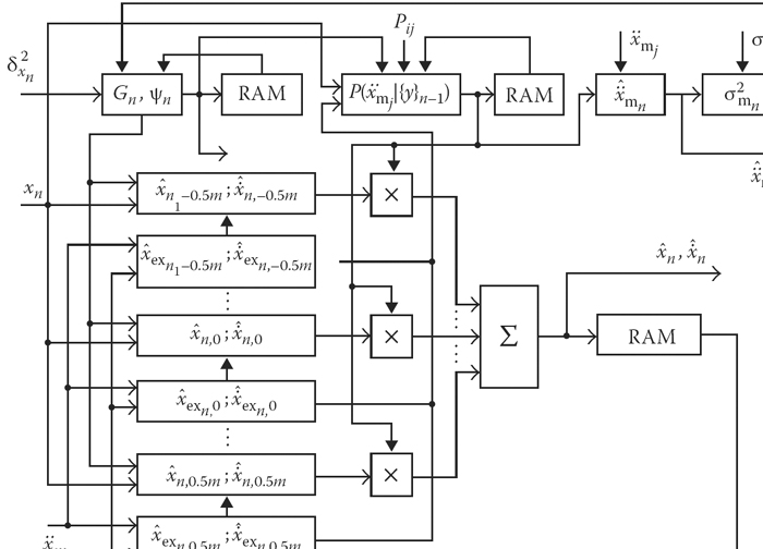
FIGURE 5.10 Adaptive filter flowchart: general case.

After that, we can define more exactly the estimations of filtered target track parameters taking into consideration the nth coordinating measure using the well-known formulas for the Kalman filter. A flowchart of the simplified adaptive filter is shown in Figure 5.11. It consists of blocks for computation of the correlation matrix of errors Ψ_n, the filter gain G_n, and the probabilities $P ({\ddot{x}}_{m_{j n}} | {Y}_{n})$ that are shared by the filter as a whole; the block to compute the estimations ${\hat{x}}_{n}$ and ${\hat{\dot{x}}}_{n}$ of target track parameters; (m + 1)th blocks of target track parameter extrapolation for each fixed magnitude of acceleration ${\ddot{x}}_{m_{j n}};$ the weight device to compute averaged extrapolated coordinates. From Figure 5.11, it is easy to understand the interaction of all blocks. Employment of adaptive filters allows us to decrease essentially the dynamic error of filtering the target track parameters within the limits of the target maneuver range. In doing so, when there is no target maneuver, the root-mean-square magnitude of random filtering error is slightly increased, on average 10%–15%.

The relative dynamic errors of filtering on the coordinate x by the adaptive filter (solid lines) and nonadaptive filter (dashed lines) with $σ_{\ddot{x}}^{2} = 0.5 g$ for the target track shown in the right top are presented in Figure 5.12. The target makes a maneuver with accelerations d₁ = 4g and d₁ = 6g, where g is the gravitational acceleration, moving with the constant velocity V_tg = 300 m/s. Maneuver is observed within the limits of six scanning periods of the radar antenna. In the case of the adaptive filter, ${\ddot{x}}_{1} = - 8 g$ , ${\ddot{x}}_{2} = 0$ , and ${\ddot{x}}_{3} = 8 g$ are considered as the discrete magnitudes of acceleration. As follows from Figure 5.12, the adaptive filter allows us to decrease the dynamic error of filtering twice in comparison with the nonadaptive filter even in the case of low-accuracy fragmentation of the possible acceleration range. In the case considered in Figure 5.12, these errors do not exceed the variance of errors under the coordinating measurement. There is a need to take into consideration that the labor intensiveness of the considered adaptive filter realization by the number of arithmetic operations is twice higher in comparison with the labor intensiveness of the nonadaptive filter realization. With an increase in the number m of discrete values of maneuver acceleration (fragmentation with high accuracy) within the limits of the range $(- {\ddot{x}}_{\max} \dots {\ddot{x}}_{\max})$ , the labor intensiveness of the considered adaptive filter realization is essentially increased.

Images

FIGURE 5.11 Flowchart of simplified adaptive filter.

Images

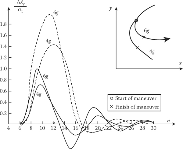
FIGURE 5.12 Dynamic errors of filtering: the adaptive filter (solid line) and nonadaptive filter (dashed line).

5.7 Logical Flowchart of Complex Radar Signal Reprocessing Algorithm

We discussed all the main operations of the radar signal reprocessing algorithms in Chapters 4 and 5. Now we consider a problem of discussed algorithm union in the unified complex algorithm of radar signal reprocessing assigned to solve the target detection problems, target tracking and filtering of target track parameters for multiple targets, and information about the contents in radar target pips coming in from the radar signal preprocessing processor output. Under consideration of the unified complex algorithm, we assume that this algorithm is assigned for radar signal reprocessing by the CRS with omnidirectional and uniform rotation radar antenna scanning. In addition, we assume that overlapping of gate signal is absent owing to target and noise environment. We assume that the realization of the unified complex algorithm is carried out by a specific computer subsystem. Random access memory (RAM) of this computer subsystem has specific data array area to store: target tracking trajectory (the data array $D_{tg}^{track}$ ); detected target tracks, that is, beginnings of target trajectories with respect to which the final decision about target tracking or cancellation is not made yet (the data array $D_{tg}^{decision}$ ); and initial points of new target tracks (the data array $D_{tg}^{intial}$ ). Each data array, in turn, has two equal zones: the first zone is to store information used within the limits of the current radar antenna scanning period and the second zone is to store information accumulated to process it within the limits of the next radar antenna scanning. Information recording for each zone is carried out in an arbitrary way.

Images

FIGURE 5.13 Logical flowchart of possible version of the united complex algorithms of radar signal reprocessing.

At first, an accessory of a new target pip to the trajectory of tracking target is checked (block 3). If this target pip belongs to a future gate of one of the tracking target trajectories, then it is considered as belonging to this trajectory and registered for this target track. Further, taking into consideration the coordinates of the new target pip, we make more exact the parameters of target track (block 4). For this purpose, one of the algorithms discussed in the this chapter is used. As a rule, this is the algorithm ensuring a filtering of maneuvering target track parameters, since the output information is used in the interests of the user (block 5). After completing the operations carried out by block 5, the processing of the next target pip is finished and the algorithm goes to choose a new target pip from the buffer.
If a new target pip does not fall into the gate of any trajectory of a tracking target, in this case, this target pip is checked for a target track belonging to any detected trajectory (block 6). For this purpose, the target pip belonging to future gates formed by results of beginnings of new target tracks is checked. If the target pip belongs to the periodical gate selected from the data array $D_{tg}^{decision}$ of detected trajectories, then this target pip is considered as an extension of this target track. Taking into consideration the coordinates of the new target pip, we make more exact the parameters of the detected tracking target trajectory (block 7). After that, we check a detection criterion and the target track is recorded into the target track array and the algorithm goes to process the next target pip.
If a new target pip belongs to no one gates of detected trajectories of tracking targets, then this target pip is checked to belong to the gates of initial lock-in formed around the individual target pips considered at the previous stages as beginnings of possible new trajectories of tracking targets (block 9). If a new target pip belongs to a regular initial lock-in gate from the data array $D_{tg}^{initial}$ , then we compute initial values of target track parameters by two target pips, that is, the algorithm of beginning a new trajectory of tracking target is realized (block 10). This beginning is transferred to the data array $D_{tg}^{decision}$ , and the algorithm starts to process the next target pip.
If a new target pip does not belong to any initial lock-in gates, then it is recorded into the data array $D_{tg}^{initial}$ as a possible beginning of a new tracking target trajectory.

Thus, under an adopted structure to process new target pips (to form beginnings of tracking target trajectory) a cycle of single realization of the considered algorithm is the random variable, statistical characteristics of which are discussed in the next chapters. In conclusion, we note that the discussed flowchart of the unified complex radar signal reprocessing algorithm is not typical, that is, acceptable for all practical situations. This is only an example allowing us to make some calculations during further analysis.

5.8 Summary and Discussion

There are many sources of error in radar-tracking performance. Fortunately, most are insignificant except for very high-precision tracking-radar applications such as range instrumentation, where the angle precision required may be on the order 0.05 mrad (mrad, or milliradian, is one thousandth of a radian, or the angle subtended by 1-m cross range at 1000-m range). Many sources of error can be avoided or reduced by radar design or modification of the tracking geometry. Cost is a major factor in providing high-precision tracking capability. Therefore, it is important to know how much error can be tolerated, which sources of error affect the application, and what are the most cost-effective means to satisfy the accuracy requirements. Because tracking radar subsystems track targets not only by angle but also in range and sometimes in Doppler, the errors in each of these target parameters must be considered in most error budgets. It is important to recognize the actual CRS information output. For a mechanically moved antenna, the angle-tracking output is usually obtained from the shaft position of the elevation and azimuth antenna axes. Absolute target location relative to their coordinates will include the accuracy of the survey of the antenna pedestal site.

The motions of a target with respect to the CRS causes the total echo signal to change with time, resulting in random fluctuations in the radar measurements of the parameters of the target. These fluctuations caused by the target only, excluding atmospheric effects and radar receiver noise contributions, are called the “target noise.” This discussion of target noise is based largely on aircraft, but it is generally applicable to any target, including land targets of complex shape that are large with respect to a wavelength. The major difference is in the target motion, but the discussions are sufficiently general to apply to any target situation. The target track model given by (5.1) must take into consideration, first of all, the target track parameter disturbance caused by a nonuniform environment, in which the target moves, atmospheric conditions, and, also, inaccuracy and inertness of control and target parameter stabilization system in the course of target moving. We may term this target track parameter disturbance as the control noise, that is, the noise generated by the target control system. As a rule, the control noise is presented as the discrete white noise with zero mean and the variance $σ_{n}^{2}$ . In addition to the control noise, the target track model must take into consideration specific disturbances caused by unpredictable changes in target track parameters that are generated by target in-flight maneuvering. We call these disturbances the target maneuver noise. In a general case, the target maneuver noise is neither white noise nor Gaussian noise.

In the solution of the filtering problems, additionally to the target track model there is a need to specify a function between the m-dimensional vector of measured coordinates Y_n and s-dimensional vector of estimated parameters θ_n at the instant of nth measuring. This function, as a rule, is given by a linear equation. In the considered case, the observed coordinates are the current target coordinates in a spherical coordinate system, the target range r_n, the azimuth β_n, and the elevation ε_n, or some specific coordinates for the CRS and radar coordinates, for example, the radar range, cosine between the radar antenna array axis and direction to the target. In some CRSs, the radial velocity ${\dot{r}}_{n}$ can serve as the measured coordinate. We note that the target track model jointly with the model of measuring process forms the model of united dynamic system representing a process subjected to filtering.

In accordance with developed procedures and methods to carry out statistical tests in mathematical statistics, the following approaches are possible to calculate the a posteriori pdf and, consequently, to estimate the parameters: the batch method when the fixed samples are used and the recurrent algorithm consisting in sequent accurate definition of the a posteriori pdf after each new measuring. Using the first approach, the a priori pdf of the estimated parameter must be given. Under the use of the second approach, the predicted pdf based on data obtained at the previous step is used as the a priori pdf on the next step. Recurrent computation of the a posteriori pdf of estimated parameter, when a correlation between the model noise and measuring errors is absent, is carried out by the formula (5.17). In a general case of nonlinear target track models and measuring process models, computations by the formula (5.17) are impossible, as a rule, in closed forms. Because of this, under solution of filtering problems in practice, various approximations of models and statistical characteristics of CRS noise and measuring processes are used. Methods of linear filtering are widely used in practice. Models of system state and measuring of these methods are supposedly linear, and the noise is considered as the Gaussian noise.

In the course of discussion of linear filtering algorithms and extrapolation under the fixed sample size of measurements, we consider several types of target track, namely, (a) the linear target track, (b) the polynomial target track, and (c) the second-order polynomial target track. Additionally, we consider the algorithm of extrapolation of target track parameters and dynamic errors of target track parameter estimation. The likelihood function of the vector parameter θ_N estimated by sequent measurements {Y_N} is given by (5.25). The vector likelihood equation is presented by (5.27). In a general case, the final solution of likelihood equation for correlated measure errors is defined by (5.29). Potential errors of target track parameters estimated by the polynomial target track model can be obtained using a linearization of the likelihood equation (5.27). The final form of the correlation matrix of errors of target track parameter estimations can be presented by (5.33). The variance of error of the smoothed coordinate estimation using three uniformly precise measurements is equal to 5/6 of the variance of individual measurement error. The variance of error of the coordinate increment estimation is only one half of the variance of error of individual measurement error owing to inaccurate target velocity estimation, and the correlation moment of relation between the errors of coordinate estimation and its increment is equal to one half of the variance of error of individual coordinate measurement. Figure 5.3 represents a coefficient of accuracy under determination of the normalized elements of correlation error matrix of linear target track parameter estimation versus the number of measurements. As follows from Figure 5.3, to obtain the required accuracy of estimations there is a need to carry out a minimum of 5–6 measurements. Turning to the algorithms of linear target track parameter estimations (5.43) and (5.44), we can easily see that these algorithms are the algorithms of nonrecursive filters and the weight coefficients $η_{\hat{x}} (i)$ and $η_{Δ_{1} \hat{x}} (i)$ form a sequence of impulse response values of these filters. To apply filter processing using these filters, there is a need to carry out N multiplications between the measured coordinate values at each step, that is, after each coordinate measurement, and the corresponding weight coefficients and, additionally, N summations of the obtained partial products. To store in memory device (N − 1) records of previous measurements, there is a need to use high-capacity memory. As a result, to realize such a filter, taking into account that N > 5, there is a need to use high-capacity memory and this realization is complex. Formulas (5.70) through (5.75) show that in the case of equally discrete and uniformly precise measurements, the optimal estimation of target second-order polynomial track parameters is determined by the weighted summing of measured coordinate values. The weight coefficients are the functions of the sample size N and the sequence number of sample i in the processing series. The coefficient of accuracy under determination of the normalized elements of correlation error matrix of target second-order polynomial track parameter estimation versus the number of measurements is shown in Figure 5.4. Comparison of diagonal elements of the matrix (5.80) that are characteristics of accuracy under estimation of the second-order polynomial target track coordinate and the first increment with analogous elements of the correlation error matrix of target linear track parameter estimation (see Figure 5.3) shows that at low values of N the accuracy of target linear track parameter estimation is much higher in comparison with the accuracy of target second-order polynomial track parameter estimation. Consequently, within the limits of small observation intervals it is worthwhile to present the target track as using the first-order polynomial. In this case, a high quality of cancellation of random errors of target track parameter estimation by filtering is guaranteed. Dynamical errors arising owing to mismatching of target movement hypotheses can be neglected as a consequence of the narrow approximated part of the target track.

The extrapolation problem of target track parameters is to define the target track parameter estimations at the point that is outside the observation interval using the magnitudes of target track parameters determined during the last observation or using a set of observed coordinate values. Under polynomial representation of an independent coordinate, the target track parameters extrapolated using the time τ_ex are defined by (5.81) through (5.83), which allow us to define the extrapolated coordinates for each specific case of target track representation. The error correlation matrix of target linear track parameter extrapolation at equally discrete coordinate measurement is given by (5.90). If the independent target track parameter coordinate is represented by the polynomial of the second order, the target track parameter extrapolation formulas and the error correlation matrix of target linear track parameter extrapolation are obtained in an analogous method.

Inconsistency between the polynomial model and nonlinear character in changing the vector of estimated target track parameters leads to dynamic errors in smoothing that can be presented in the form of differences between the true value of the vector of estimated target track parameters and the mathematical expectation of the vector estimate. To describe the dynamic errors of estimations of the target track parameters by algorithms that are synthesized by the maximum likelihood criterion and using the target track polynomial model, we employ the well-known theory of errors at approximation of arbitrary continuously differentiable function f(t) within the limits of the interval t_N − t₀ by the polynomial function of the first or second order using the technique of least squares. Comparison of the dynamical errors of approximation of the polar coordinates by the polynomials of the first and second power at the same values of target track parameters V_tg, r_min, T_eq and the sample size (N − 1)T_eq shows us that the dynamic errors under linear approximation are approximately one order higher than under quadratic approximation. Moreover, under approximation of r_tg(t) and β_tg(t) by the polynomials of the second power, the dynamic errors are small in comparison with random errors and we can neglect them. However, as shown by simulation, if the target is in an in-flight maneuver and the CRS is moving, the dynamic errors are essentially increased, because nonlinearity in changing the polar coordinates is increased sharply at the same time.

Methods of estimation of the target track parameters based on the fixed sample of measured coordinate, which are discussed in the previous sections, are used, as a rule, at the beginning of the detected target trajectory. Implementation of these methods in the course of tracking is not worthwhile owing to complexity and insufficient accuracy defined by the small magnitude of employed measures. Accordingly, there is a need to employ the recurrent algorithms ensuring a sequential, that is, after each new coordinating measurement, adjustment of target track parameters with their filtering purposes. At the recurrent filter output, we obtain the target track parameter estimations caused by the last observation. By this reason, a process of recurrent evaluation is further called sequential filtering, and corresponding algorithms are called the algorithms of sequential filtering of target track parameters.

In a discussion of the recurrent filtering algorithms, we obtain that the optimal recurrent linear filtering algorithm is defined by the Kalman filtering equations. A discrete optimal recurrent filter possesses the following properties: (a) filtering equations have recurrence relations and can be realized well by the computer system; (b) filtering equations simultaneously represent a description of procedure to realize this filter, and in doing so, a part of the filter is similar to the model of target track (compare Figures 5.2 and 5.6); (c) the error correlation matrix of target track parameter estimation Ψ_n is computed independently of measuring Y_n; consequently, if statistical characteristics of measuring errors are given then the correlation matrix Ψ_n can be computed in advance and stored in a memory device; this essentially reduces the time of realization of target track parameter filtering.

As we can see from Figure 5.7, with an increase in n the filter gains in the coordinate and velocity are approximated asymptotically to zero. Consequently, with an increase in n the results of last measurements at filtering the coordinate and velocity are taken into consideration with less weight, and the filtering algorithm ceases to respond to changes in the input signal. Moreover, essential problems under realization of the filter arise in computer systems with a limited capacity of number representation. At high n, the computational errors are accumulated and commensurable with a value of the lower order of computer system that leads to losses in conditionality and positive determinacy of the correlation matrices of extrapolation errors and filtering of the target track parameters. The “filter divergence” phenomenon, when the filtering errors are increased sharply and the filter stops to operate, appears. Thus, if we do not take specific measures in correction, the optimal linear recurrent filter cannot be employed in complex automatic radar systems. To overcome this problem is a great advance in automation of CRSs.

In a general form, the problem of recurrent filter stabilization is the problem of ill-conditioned problem solution, namely, the problem in which small deviations in initial data cause arbitrarily large but finite deviations in solution. The method of stable (approximated) solution was designed for ill-conditioned problems. This method is called the regularization or smoothing method. In accordance with this method, there is a need to add the matrix αI to the matrix of measuring errors R_n given by (5.127), where I is the identity matrix, under the synthesis of a regularizing algorithm of optimal filtering of the unperturbed dynamic system parameters (5.134). A general approach to obtain the stable solutions by the regularization or smoothing method is the artificial rough rounding of measuring results. However, the employment of this method in a pure form is impossible since a way to choose the regularization parameter a, is generally unknown. In practice, a cancellation of divergence of the recurrent filter can be ensured by effective limitation of memory device capacity including in the recurrent filter. In line with this, we consider several cases. For example, in the case of introduction of an additional term into the correlation matrix of extrapolation errors we obtain that the recurrent filter with an additional term approximates the filter with finite memory capacity at the corresponding choice of the coefficients c₀, c₁…, c_s. Under introduction of artificial aging of measuring errors and equally discrete and uniformly precise coordinating measurements, the smoothing coefficients of the filter are converged to positive constants in the filter safe operating area. However, it is impossible to find the parameter s for this filter so that the variance and dynamic errors of these filters and the filter with finite memory capacity are matched. In the case of gain lower bound for the simplest case of the equally discrete and uniformly precise coordinating measurements, the gain bound is defined directly by the formulas for G_n at the given effective memory capacity of the filter. Computation and simulation show that the last procedure is the best way by criterion of realization cost and rate to define the variances of errors under the equally discrete and uniformly precise coordinating measurements from considered procedures to limit the recurrent filter memory capacity. The first procedure, that is, the introduction of an additional term into the correlation matrix of extrapolation errors, is a little worse. The second procedure, that is, an introduction of the multiplicative term into the correlation matrix of extrapolation errors, is worse in comparison with the first and third ones by realization costs and rate of convergence of the error variance to the constant magnitude.

In the consideration of filtering methods and algorithms of target track parameters, we assume that the model equation of target track corresponds to the true target moving. In practice, this correspondence is absent, as a rule, owing to the target maneuvering. One requirement of successful solution of problems concerning the real target track parameter filtering is to take into consideration a possible target maneuver. The state equation of maneuvering target is given by (5.144). According to precision of CRS characteristics and estimated target maneuver, three approaches are possible for designing the filtering algorithm of real target track parameters: (a) the target has limited possibilities for maneuver, for example, there are only random unpremeditated disturbances in the target track (there is a need to note that the methods discussed in the previous section to limit a memory capacity of the recurrent filter by their sense and consequences are equivalent to the considered method to record the target maneuver since a limitation in memory capacity of the recurrent filter, increasing a stability, can simultaneously decrease the sensitivity of the filter to short target maneuvering); (b) we assume that the target performs only a single premeditated maneuver of high intensity within the observation time interval; in this case, the target track can be divided into three parts: before starting, in the course of, and after finishing the target maneuver, as the intensity vector of target maneuver at the instants of start and finish of target maneuvering are subjected to statistical estimation in this case by totality of input signals (measuring coordinates); consequently, in the given case, the filtering problem is reduced to designing a switching filtering algorithm or switching filter with switching control based on analysis of input signals; this algorithm concerns a class of simple adaptive algorithms with a self-training system; (c) it is assumed that the targets subjected to tracking have good maneuvering abilities and are able to perform a set of maneuvers within the limits of observation time; these maneuvers are related to air miss relative to other targets or flight in the given space; in this case, to design the formula flowchart of filtering algorithms of target track parameters there is a need to have data about the mathematical expectation $E (g_{m_{n}})$ and the variance $σ_{g}^{2}$ of target maneuver intensity for each target and within the limits of each interval of information updating; these data (estimations) can be obtained only based on an input information analysis, and the filtering is realized by the adaptive recurrent filter.

The problems of target maneuver detection or definition of the probability to perform a maneuver by target are solved in one form or another by adaptive filtering algorithms. Detection of target maneuver is possible by deviation of target track from a straight-line trajectory by each filtered target track coordinate. However, in a spherical coordinate system, when the coordinates are measured by a CRS, the trajectory of any target, even in the event that the target is moving uniformly and in straight line, is defined by nonlinear functions. For this reason, a detection and definition of target maneuver characteristics under filtering of target track parameters using the spherical coordinate system are impossible. To solve the problem of target maneuver detection and based on other considerations, it is worthwhile to carry out a filtering of the target track parameters using the Cartesian coordinate system with the origin in the CRS location. This coordinate system is called the local Cartesian coordinate system. The formulas of coordinate transformation from the spherical coordinate system to the local Cartesian one are given by (5.149). Transformation to the local Cartesian coordinate system leads to an appearance of nonuniformly precise correlation between the coordinates at the filter input, which, in turn, leads to the complexity of filter structure and additional computer cost under realization. Also, there is a need to take into consideration that other operations of signal reprocessing by a CRS, for example, target pip gating, target pip identification, and so on, are realized in the simplest form in the spherical coordinate system. Therefore, the filtered target track parameters must be transformed from the local Cartesian coordinate system to the spherical one during each step of target information update. Thus, to solve the problem of adaptive filtering of the track parameters of maneuvering targets it is worth employing the recurrent filters, where the filtered target track parameters are represented in the Cartesian coordinate system and comparison between the measured and extrapolated coordinates is carried out in the spherical coordinate system. In this case, the detection of target maneuver or definition of the probability performance of target maneuver can be organized based on analysis of deviation of the target track parameter estimations from magnitudes corresponding to the hypotheses of straight-line and uniform target moving.

There is a statistical dependence between estimations of target track parameters by all coordinates in the considered recurrent filter. This fact poses difficulties in obtaining the target track parameter estimations and leads to tightened requirements for CRS computer subsystems. We can decrease the computer cost refusing from optimal filtering of target track parameters, making the filter simple. In particular, a primitive simplification is a rejection of joint filtering of target track parameters and passage to individual filtering of Cartesian coordinates with subsequent transformation of obtained target track parameter estimation coordinates to the polar coordinate system. The procedure of simplified filtering version is discussed. Comparison of accuracy characteristics of optimal and simple filtering procedures with double transformation of coordinates is carried out by simulation. For example, the dependences of root-mean-square error magnitudes of target track azimuth coordinate versus the number of measurements (the target track is indicated in the right top corner) for optimal (curve 1) and simple (curve 2) filtering algorithms at r_min = 10 and 20 km are shown in Figure 5.9. In Figure 5.9, we see that in the case of a simple filter, accuracy deteriorates from 5–15% against target range, course, speed, and the number of observers. At r_min < 10 km, this deterioration in accuracy is about 30%. However, the computer cost is decreased approximately one order.

Under adaptive filtering, the linear dynamic system described by the state equation given by (5.144) is considered as the target track model. Target track distortions caused by a deliberate target maneuver are represented as a random process, the mean $E (g_{m_{n}})$ of which is changed step-wise taking a set of fixed magnitudes (states) within the limits of range $[- g_{m_{\max}}, + g_{m_{\max}}]$ . Transitions of step-wise process from the state i to the state j are carried out with the probability P_ij ≥ 0 defined by a priori data about the target maneuver. The time when the process is in the state i before transition into the state j is the random variable with arbitrary pdf p(t_i). The mathematical model is the semi-Markov random process. Distortions of the target track caused by a deliberate target maneuver and errors of intensity estimations of deliberate target maneuver are characterized by the random component η_n in adaptive filtering algorithm. The matrices Φ_n, Γ_n, and K_n are considered as known. Initially, we consider the Bayesian approach to design the adaptive filtering algorithm for the case of continuous distortion action $g_{m_{n}}$ .

As is well known, an optimal estimation of the parametric vector θ_n at the quadratic loss can be defined from (5.170). The problem to estimate the vector ${\hat{θ}}_{n}$ is reduced to weight averaging the estimations ${\hat{θ}}_{n} (g_{m_{n}})$ that are the solution of filtering problem at the fixed magnitudes of $g_{m_{n}}$ . The estimations ${\hat{θ}}_{n} (g_{m_{n}})$ can be obtained by any way that minimizes the MMSE criterion including the recurrent linear filter or Kalman filter. The problem of optimal adaptive filtering will be solved when the a posteriori pdf $p (g_{m_{n}} | {Y}_{n})$ is determined at each step. Determination of this pdf by a sample of measurements {Y}_n and its employment with the purpose to obtain the weight estimations is the main peculiarity of the considered adaptive filtering method.

A flowchart of the adaptive filter realizing the described system of equations is shown in Figure 5.10. The adaptive filter consists of (m + 1) Kalman filters connected in parallel and each of them is tuned on one of possible discrete values of parametric disturbance. The resulting estimation of filtered target track parameters is defined as the weight summation of conditional estimations at the outputs of these elementary filters. The weight coefficients $P ({\ddot{x}}_{m_{j n}} | {Y}_{n})$ are made more exact at each step, that is, after each measurement of the coordinate x using the recurrent formula (5.186). Blocks for computation of the correlation matrix Ψ_n of errors of target track parameter estimation and filter gain G_n are shared for all elementary filters. Therefore, the complexity of realization of the considered adaptive filter takes place owing to (m + 1) multiple computations of extrapolated and smoothed magnitudes of filtered target track parameters and computation of the weights $P ({\ddot{x}}_{m_{j n}} | {Y}_{n})$ at each step of updating the target information.

The adaptive filter design based on the principle of weight of partial estimations can be simplified carrying out the weight of extrapolated values only of filtered target track parameters, and using this weight, to compute the filtered target track parameters by the usual (undivided) filter instead of weighting the output estimations of filtered target track parameters. The equation system of the simplified adaptive filter differs from the previous one by the fact that the extrapolated values of filtered target track parameters determined by (5.180) are averaged with the definite weights. After that we can define more exactly the estimations of filtered target track parameters taking into consideration the nth coordinate measure using the well-known formulas for the Kalman filter.

As follows from Figure 5.12, the adaptive filter allows us to decrease the dynamic error of filtering twice in comparison with the nonadaptive filter even in the case of low-accuracy fragmentation of possible acceleration range. In the case considered in Figure 5.12, these errors do not exceed the variance of errors under coordinating measurement. There is a need to take into consideration that the labor intensiveness of the considered adaptive filter realization by the number of arithmetic operations is twice higher in comparison with the labor intensiveness of the nonadaptive filter realization. With an increase in the number m of discrete values of maneuver acceleration (fragmentation with high accuracy) within the limits of the range $(- {\ddot{x}}_{\max} \dots {\ddot{x}}_{\max})$ , the labor intensiveness of the considered adaptive filter realization is essentially increased.

A logical flowchart of a possible version of the unified complex radar signal reprocessing algorithm is shown in Figure 5.13. In accordance with this block diagram, each new target pip selected from the buffer after coordinate transformation into the Cartesian coordinate system is subjected to the definite stages of signal processing discussed in this chapter. Under an adopted structure to process new target pips (to form beginnings of tracking target trajectories), a cycle of a single realization of the considered algorithm is the random variable, statistical characteristics of which will be discussed in the next chapters. In conclusion, we note that the discussed flowchart of the unified complex radar signal reprocessing algorithm is not typical, that is, acceptable for all practical situations. This is only an example allowing us to make some calculations during further analysis.

References

1. Milway, W. B. 1985. Multiple targets instrumentation radars for military test and evaluation, in Proceedings International Telemetry Council, October 28–31, Las Vegas, Nevada, Vol. XXI, pp. 625–631.

2. Stegall, R.L. 1987. Multiple object tracking radar: System engineering considerations, in Proceedings International Telemetry Council, October 26–29, San Diego, California, Vol. XXIII, pp. 537–544.

3. Noblit, R. S. 1967. Reliability without redundancy from a radar monopulse receiver. Microwave, 12: 56–60.

4. Sakamoto, H. and P. Z. Peeblez. 1978. Monopulse radar. IEEE Transactions on Aerospace and Electronic Systems, 14(1): 199–208.

3. Stark, H. and J. W. Woods. 2002. Probability and Random Processes with Applications to Signal Processing. 3rd Edn. Upper Saddle River, NJ: Prentice-Hall, Inc.

6. Thomas, M. C. and J. A. Thomas. 2006. Elements of Information Theory. 2nd Edn. New York: John Wiley & Sons, Inc.

7. Rappaport, T. S. 2002. Wireless Communications Principles and Practice. Upper Saddle River, NJ: Prentice Hall, Inc.

8. Kay, S. 2006. Intuitive Probability and Random Processes Using Matlab. New York: Springer, Inc.

9. Castella, F. R. 1974. Analytical results for the x, y Kalman tracking filter. IEEE Transactions on Aerospace and Electronic Systems, 10(11): 891–894.

10. Kalman, R. E. 1960. A new approach to linear filtering and prediction problem. Journal of Basic Engineering (ASME Transactions, Ser. D), 82: 35–45.

11. Kalman, R.E. and R. S. Bucy. 1961. New results in linear filtering and prediction theory. Journal of Basic Engineering (ASME Transactions, Ser. D), 83: 95–107

12. Sorenson, H. 1970. Least-squares estimation: From Gauss to Kalman. IEEE Spectrum, 7: 63–68.

13. Stewart, R.W. and R. Chapman. 1990. Fast stable Kalman filter algorithm utilizing the square root, in Proceedings International Conference on Acoustics, Speech and Signal Processing, April 3–6, Albuquerque, New Mexico, pp. 1815–1818.

14. Lin, D.W. 1984. On the digital implementation of the fast Kalman algorithm. IEEE Transactions on Acoustics, Speech and Signal Processing, 32: 998–1005.

15. Bozic, S. M. 1994. Digital and Kalman Filtering. 2nd Edn. New York: Halsted Press, Inc.

16. Bellini, S. 1977. Numerical comparison of Kalman filter algorithms: Orbit determination case study. Automatica, 13: 23–35.

17. Tikhonov, A.N. and V.Ya. Arsenin. 1979. Methods of Solution for Ill-Conditioned Problems. Moscow, Russia: Science, Inc.

18. Rybova-Oreshkova, A. P. 1974. Investigations of recurrent filters with limited memory capacity. News of Academy of Sciences of the USSR Series. Engineering Cybernetics, 5: 173–187.

19. Sayed, A. 2003. Fundamentals of Adaptive Filtering. New York: Wiley Interscience/IEEE Press, Inc.

..................Content has been hidden....................

You can't read the all page of ebook, please click here login for view all page.

Table of Contents for Chapter 5 Filtering and Extrapolation of Target Track Parameters Based on Radar Measure

Create new playlist

Sign In

Sign Up

Table of Contents for
Chapter 5 Filtering and Extrapolation of Target Track Parameters Based on Radar Measure