
Chapter 4
Black Box Testing
In this chapter—
4.1 WHAT IS BLACK BOX TESTING?
Black box testing involves looking at the specifications and does not require examining the code of a program. Black box testing is done from the customer's viewpoint. The test engineer engaged in black box testing only knows the set of inputs and expected outputs and is unaware of how those inputs are transformed into outputs by the software.
Black box testing is done without the knowledge of the internals of the system under test.
Black box tests are convenient to administer because they use the complete finished product and do not require any knowledge of its construction. Independent test laboratories can administer black box tests to ensure functionality and compatibility.
Let us take a lock and key. We do not know how the levers in the lock work, but we only know the set of inputs (the number of keys, specific sequence of using the keys and the direction of turn of each key) and the expected outcome (locking and unlocking). For example, if a key is turned clockwise it should unlock and if turned anticlockwise it should lock. To use the lock one need not understand how the levers inside the lock are constructed or how they work. However, it is essential to know the external functionality of the lock and key system. Some of the functionality that you need to know to use the lock are given below.
With the above knowledge, you have meaningful ways to test a lock and key before you buy it, without the need to be an expert in the mechanics of how locks, keys, and levers work together. This concept is extended in black box testing for testing software.

| Functionality | What you need to know to use |
|---|---|
| Features of a lock | It is made of metal, has a hole provision to lock, has a facility to insert the key, and the keyhole ability to turn clockwise or anticlockwise. |
| Features of a key | It is made of metal and created to fit into a particular lock's keyhole. |
| Actions performed | Key inserted and turned clockwise to lock Key inserted and turned anticlockwise to unlock |
States
Inputs Expected outcome |
Locked Unlocked Key turned clockwise or anticlockwise Expected outcome Locking Unlocking |
Black box testing thus requires a functional knowledge of the product to be tested. It does not mandate the knowledge of the internal logic of the system nor does it mandate the knowledge of the programming language used to build the product. Our tests in the above example were focused towards testing the features of the product (lock and key), the different states, we already knew the expected outcome. You may check if the lock works with some other key (other than its own). You may also want to check with a hairpin or any thin piece of wire if the lock works. We shall see in further sections, in detail, about the different kinds of tests that can be performed in a given product.
4.2 WHY BLACK BOX TESTING
Black box testing helps in the overall functionality verification of the system under test.
Black box testing is done based on requirements It helps in identifying any incomplete, inconsistent requirement as well as any issues involved when the system is tested as a complete entity.
Black box testing addresses the stated requirements as well as implied requirements Not all the requirements are stated explicitly, but are deemed implicit. For example, inclusion of dates, page header, and footer may not be explicitly stated in the report generation requirements specification. However, these would need to be included while providing the product to the customer to enable better readability and usability.
Black box testing encompasses the end user perspectives Since we want to test the behavior of a product from an external perspective, end-user perspectives are an integral part of black box testing.
Black box testing handles valid and invalid inputs It is natural for users to make errors while using a product. Hence, it is not sufficient for black box testing to simply handle valid inputs. Testing from the end-user perspective includes testing for these error or invalid conditions. This ensures that the product behaves as expected in a valid situation and does not hang or crash when provided with an invalid input. These are called positive and negative test cases.
The tester may or may not know the technology or the internal logic of the product. However, knowing the technology and the system internals helps in constructing test cases specific to the error-prone areas.
Test scenarios can be generated as soon as the specifications are ready. Since requirements specifications are the major inputs for black box testing, test design can be started early in the cycle.
4.3 WHEN TO DO BLACK BOX TESTING?
Black box testing activities require involvement of the testing team from the beginning of the software project life cycle, regardless of the software development life cycle model chosen for the project.
Testers can get involved right from the requirements gathering and analysis phase for the system under test. Test scenarios and test data are prepared during the test construction phase of the test life cycle, when the software is in the design phase.
Once the code is ready and delivered for testing, test execution can be done. All the test scenarios developed during the construction phase are executed. Usually, a subset of these test scenarios is selected for regression testing.
4.4 HOW TO DO BLACK BOX TESTING?
As we saw in Chapter 1, it is not possible to exhaustively test a product, however simple the product is. Since we are testing external functionality in black box testing, we need to arrive at a judicious set of tests that test as much of the external functionality as possible, uncovering as many defects as possible, in as short a time as possible. While this may look like a utopian wish list, the techniques we will discuss in this section facilitates this goal. This section deals with the various techniques to be used to generate test scenarios for effective black box testing.
Black box testing exploits specifications to generate test cases in a methodical way to avoid redundancy and to provide better coverage.
The various techniques we will discuss are as follows.
- Requirements based testing
- Positive and negative testing
- Boundary value analysis
- Decision tables
- Equivalence partitioning
- State based testing
- Compatibility testing
- User documentation testing
- Domain testing
4.4.1 Requirements Based Testing
Requirements testing deals with validating the requirements given in the Software Requirements Specification (SRS) of the software system.
As mentioned in earlier chapters, not all requirements are explicitly stated; some of the requirements are implied or implicit. Explicit requirements are stated and documented as part of the requirements specification. Implied or implicit requirements are those that are nor documented but assumed to be incorporated in the system.
The precondition for requirements testing is a detailed review of the requirements specification. Requirements review ensures that they are consistent, correct, complete, and testable. This process ensures that some implied requirements are converted and documented as explicit requirements, thereby bringing better clarity to requirements and making requirements based testing more effective.
Some organizations follow a variant of this method to bring more details into requirements. All explicit requirements (from the Systems Requirements Specifications) and implied requirements (inferred by the test team) are collected and documented as “Test Requirements Specification” (TRS). Requirements based testing can also be conducted based on such a TRS, as it captures the testers’ perspective as well. However, for simplicity, we will consider SRS and TRS to be one and the same.
A requirements specification for the lock and key example explained earlier can be documented as given in Table 4.1.

Requirements (like the ones given above) are tracked by a Requirements Traceability Matrix (RTM). An RTM traces all the requirements from their genesis through design, development, and testing. This matrix evolves through the life cycle of the project. To start with, each requirement is given a unique id along with a brief description. The requirement identifier and description can be taken from the Requirements Specification (above table) or any other available document that lists the requirements to be tested for the product. In the above table, the naming convention uses a prefix “BR” followed by a two-digit number. BR indicates the type of testing—"Black box-requirements testing.” The two-digit numerals count the number of requirements. In systems that are more complex, an identifier representing a module and a running serial number within the module (for example, INV-01, AP-02, and so on) can identify a requirement. Each requirement is assigned a requirement priority, classified as high, medium or low. This not only enables prioritizing the resources for development of features but is also used to sequence and run tests. Tests for higher priority requirements will get precedence over tests for lower priority requirements. This ensures that the functionality that has the highest risk is tested earlier in the cycle. Defects reported by such testing can then be fixed as early as possible.
As we move further down in the life cycle of the product, and testing phases, the cross-reference between requirements and the subsequent phases is recorded in the RTM. In the example given here, we only list the mapping between requirements and testing; in a more complete RTM, there will be columns to reflect the mapping of requirements to design and code.
The “test conditions” column lists the different ways of testing the requirement. Test conditions can be arrived at using the techniques given in this chapter. Identification of all the test conditions gives a comfort feeling that we have not missed any scenario that could produce a defect in the end-user environment. These conditions can be grouped together to form a single test case. Alternatively, each test condition can be mapped to one test case.
The “test case IDs” column can be used to complete the mapping between test cases and the requirement. Test case IDs should follow naming conventions so as to enhance their usability. For example, in Table 4.2, test cases are serially numbered and prefixed with the name of the product. In a more complex product made up of multiple modules, a test case ID may be identified by a module code and a serial number.
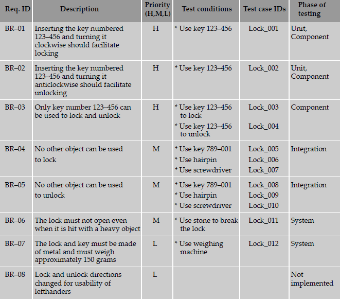
Once the test case creation is completed, the RTM helps in identifying the relationship between the requirements and test cases. The following combinations are possible.
- One to one—For each requirement there is one test case (for example, BR-01)
- One to many—For each requirement there are many test cases (for example, BR-03)
- Many to one—A set of requirements can be tested by one test case (not represented in Table 4.2)
- Many to many—Many requirements can be tested by many test cases (these kind of test cases are normal with integration and system testing; however, an RTM is not meant for this purpose)
- One to none—The set of requirements can have no test cases. The test team can take a decision not to test a requirement due to non-implementation or the requirement being low priority (for example, BR-08)
A requirement is subjected to multiple phases of testing—unit, component, integration, and system testing. This reference to the phase of testing can be provided in a column in the Requirements Traceability Matrix. This column indicates when a requirement will be tested and at what phase of testing it needs to be considered for testing.
An RTM plays a valuable role in requirements based testing.
- Regardless of the number of requirements, ideally each of the requirements has to be tested. When there are a large numbers of requirements, it would not be possible for someone to manually keep a track of the testing status of each requirement. The RTM provides a tool to track the testing status of each requirement, without missing any (key) requirements.
- By prioritizing the requirements, the RTM enables testers to prioritize the test cases execution to catch defects in the high-priority area as early as possible. It is also used to find out whether there are adequate test cases for high-priority requirements and to reduce the number of test cases for low-priority requirements. In addition, if there is a crunch for time for testing, the prioritization enables selecting the right features to test.
- Test conditions can be grouped to create test cases or can be represented as unique test cases. The list of test case(s) that address a particular requirement can be viewed from the RTM.
- Test conditions/cases can be used as inputs to arrive at a size / effort / schedule estimation of tests.
The Requirements Traceability Matrix provides a wealth of information on various test metrics. Some of the metrics that can be collected or inferred from this matrix are as follows.
- Requirements addressed prioritywise—This metric helps in knowing the test coverage based on the requirements. Number of tests that is covered for high-priority requirement versus tests created for low-priority requirement.
- Number of test cases requirementwise—For each requirement, the total number of test cases created.
- Total number of test cases prepared—Total of all the test cases prepared for all requirements.
Once the test cases are executed, the test results can be used to collect metrics such as
- Total number of test cases (or requirements) passed—Once test execution is completed, the total passed test cases and what percent of requirements they correspond.
- Total number of test cases (or requirements) failed—Once test execution is completed, the total number of failed test cases and what percent of requirements they correspond.
- Total number of defects in requirements—List of defects reported for each requirement (defect density for requirements). This helps in doing an impact analysis of what requirements have more defects and how they will impact customers. A comparatively high-defect density in low-priority requirements is acceptable for a release. A high-defect density in high-priority requirement is considered a high-risk area, and may prevent a product release.
- Number of requirements completed—Total number of requirements successfully completed without any defects. A more detailed coverage of what metrics to collect, how to plot and analyze them, etc are given in Chapter 17.
- Number of requirements pending—Number of requirements that are pending due to defects.
Requirements based testing tests the product's compliance to the requirements specifications.
A more detailed coverage of what metrics to collect, how to plot and analyze them etc are given in Chapter 17.
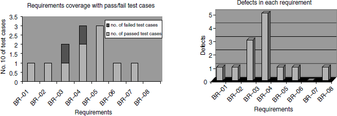
To illustrate the metrics analysis, let us assume the test execution data as given in Table 4.3.

From the above table, the following observations can be made with respect to the requirements.
- 83 percent passed test cases correspond to 71 percent of requirements being met (five out of seven requirements met; one requirement not implemented). Similarly, from the failed test cases, outstanding defects affect 29 percent (= 100 - 71) of the requirements.
- There is a high-priority requirement, BR-03, which has failed. There are three corresponding defects that need to be looked into and some of them to be fixed and test case Lock_04 need to be executed again for meeting this requirement. Please note that not all the three defects may need to be fixed, as some of them could be cosmetic or low-impact defects.
- There is a medium-priority requirement, BR-04, has failed. Test case Lock_06 has to be re-executed after the defects (five of them) corresponding to this requirement are fixed.
- The requirement BR-08 is not met; however, this can be ignored for the release, even though there is a defect outstanding on this requirement, due to the low-priority nature of this requirement.
The metrics discussed can be expressed graphically. Such graphic representations convey a wealth of information in an intuitive way. For example, from the graphs given in Figure 4.1, (coloured figure available on Illustrations) it becomes obvious that the requirements BR-03 and BR-04 have test cases that have failed and hence need fixing.
4.4.2 Positive and Negative Testing
Positive testing tries to prove that a given product does what it is supposed to do. When a test case verifies the requirements of the product with a set of expected output, it is called positive test case. The purpose of positive testing is to prove that the product works as per specification and expectations. A product delivering an error when it is expected to give an error, is also a part of positive testing.
Positive testing can thus be said to check the product's behavior for positive and negative conditions as stated in the requirement.
For the lock and key example, a set of positive test cases are given below. (Please refer to Table 4.2 for requirements specifications.)
Let us take the first row in the below table. When the lock is in an unlocked state and you use key 123—156 and turn it clockwise, the expected outcome is to get it locked. During test execution, if the test results in locking, then the test is passed. This is an example of “positive test condition” for positive testing.
In the fifth row of the table, the lock is in locked state. Using a hairpin and turning it clockwise should not cause a change in state or cause any damage to the lock. On test execution, if there are no changes, then this positive test case is passed. This is an example of a “negative test condition” for positive testing.
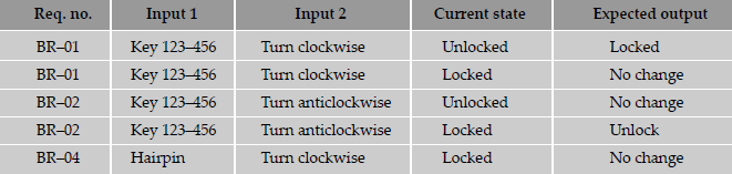
Positive testing is done to verify the known test conditions and negative testing is done to break the product with unknowns.
Negative testing is done to show that the product does not fail when an unexpected input is given. The purpose of negative testing is to try and break the system. Negative testing covers scenarios for which the product is not designed and coded. In other words, the input values may not have been represented in the specification of the product. These test conditions can be termed as unknown conditions for the product as far as the specifications are concerned. But, at the end-user level, there are multiple scenarios that are encountered and that need to be taken care of by the product. It becomes even more important for the tester to know the negative situations that may occur at the end-user level so that the application can be tested and made foolproof. A negative test would be a product not delivering an error when it should or delivering an error when it should not.
Table 4.5 gives some of the negative test cases for the lock and key example.

In the above table, unlike what we have seen in positive testing, there are no requirement numbers. This is because negative testing focuses on test conditions that lie outside the specification. Since all the test conditions are outside the specification, they cannot be categorized as positive and negative test conditions. Some people consider all of them as negative test conditions, which is technically correct.
The difference between positive testing and negative testing is in their coverage. For positive testing if all documented requirements and test conditions are covered, then coverage can be considered to be 100 percent. If the specifications are very clear, then coverage can be achieved. In contrast there is no end to negative testing, and 100 percent coverage in negative testing is impractical. Negative testing requires a high degree of creativity among the testers to cover as many “unknowns” as possible to avoid failure at a customer site.
4.4.3 Boundary Value Analysis
As mentioned in the last section, conditions and boundaries are two major sources of defects in a software product. We will go into details of conditions in this section. Most of the defects in software products hover around conditions and boundaries. By conditions, we mean situations wherein, based on the values of various variables, certain actions would have to be taken. By boundaries, we mean “limits” of values of the various variables.
We will now explore boundary value analysis (BVA), a method useful for arriving at tests that are effective in catching defects that happen at boundaries. Boundary value analysis believes and extends the concept that the density of defect is more towards the boundaries.
To illustrate the concept of errors that happen at boundaries, let us consider a billing system that offers volume discounts to customers.
Most of us would be familiar with the concept of volume discounts when we buy goods —buy one packet of chips for $1.59 but three for $4. It becomes economical for the buyer to buy in bulk. From the seller's point of view also, it is economical to sell in bulk because the seller incurs less of storage and inventory costs and has a better cash flow. Let us consider a hypothetical store that sells certain commodities and offers different pricing for people buying in different quantities—that is, priced in different “slabs.”
From the above table, it is clear that if we buy 5 units, we pay 5*5 = $25. If we buy 11 units, we pay 5*10 = $50 for the first ten units and $4.75 for the eleventh item. Similarly, if we buy 15 units, we will pay 10*5 + 5*4.75 = $73.75.

| Number of units bought | Price per unit |
|---|---|
| First ten units (that is, from 1 to 10 units) | $5.00 |
| Next ten units (that is, from units 11 to 20 units) | $4.75 |
| Next ten units (that is, from units 21 to 30 units) | $4.50 |
| More than 30 units | $4.00 |
The question from a testing perspective for the above problem is what test data is likely to reveal the most number of defects in the program? Generally it has been found that most defects in situations such as this happen around the boundaries—for example, when buying 9, 10, 11, 19, 20, 21, 29, 30, 31, and similar number of items. While the reasons for this phenomenon is not entirely clear, some possible reasons are as follows.
- Programmers’ tentativeness in using the right comparison operator, for example, whether to use the < = operator or < operator when trying to make comparisons.
- Confusion caused by the availability of multiple ways to implement loops and condition checking. For example, in a programming language like C, we have for loops, while loops and repeat loops. Each of these have different terminating conditions for the loop and this could cause some confusion in deciding which operator to use, thus skewing the defects around the boundary conditions.
- The requirements themselves may not be clearly understood, especially around the boundaries, thus causing even the correctly coded program to not perform the correct way.
In the above case, the tests that should be performed and the expected values of the output variable (the cost of the units ordered) are given in Table 4.6 below. This table only includes the positive test cases. Negative test cases like a non-numeric are not included here. The circled rows are the boundary values, which are more likely to uncover the defects than the rows that are not circled.

Boundary value analysis is useful to generate test cases when the input (or output) data is made up of clearly identifiable boundaries or ranges.
Another instance where boundary value testing is extremely useful in uncovering defects is when there are internal limits placed on certain resources, variables, or data structures. Consider a database management system (or a file system) which caches the recently used data blocks in a shared memory area. Usually such a cached area is limited by a parameter that the user specifies at the time of starting up the system. Assume that the database is brought up specifying that the most recent 50 database buffers have to be cached. When these buffers are full and a 51st block needs to be cached, the least recently used buffer—the first buffer—needs to be released, after storing it in secondary memory. As you can observe, both the operations—inserting the new buffer as well as freeing up the first buffer—happen at the “boundaries.”
As shown in Figure 4.2 below, there are four possible cases to be tested—first, when the buffers are completely empty (this may look like an oxymoron statement!); second, when inserting buffers, with buffers still free; third, inserting the last buffer, and finally, trying to insert when all buffers are full. It is likely that more defects are to be expected in the last two cases than the first two cases.

To summarize boundary value testing.
- Look for any kind of gradation or discontinuity in data values which affect computation—the discontinuities are the boundary values, which require thorough testing.
- Look for any internal limits such as limits on resources (as in the example of buffers given above). The behavior of the product at these limits should also be the subject of boundary value testing.
- Also include in the list of boundary values, documented limits on hardware resources. For example, if it is documented that a product will run with minimum 4MB of RAM, make sure you include test cases for the minimum RAM (4MB in this case).
- The examples given above discuss boundary conditions for input data—the same analysis needs to be done for output variables also.
Boundary value analysis discussed here in context of black box testing applies to white box testing also. Internal data structures like arrays, stacks, and queues need to be checked for boundary or limit conditions; when there are linked lists used as internal structures, the behavior of the list at the beginning and end have to be tested thoroughly.
Boundary values and decision tables help identify the test cases that are most likely to uncover defects. A generalization of both these concepts is the concept of equivalence classes, discussed later in this chapter.
4.4.4 Decision Tables
To illustrate the use of conditions (and decision tables) in testing, let us take a simple example of calculation of standard deduction on taxable income. The example is meant to illustrate the use of decision tables and not to be construed as tax advice or a realistic tax scenario in any specific country.
Most taxpayers have a choice of either taking a standard deduction or itemizing their deductions. The standard deduction is a dollar amount that reduces the amount of income on which you are taxed. It is a benefit that eliminates the need for many taxpayers to itemize actual deductions, such as medical expenses, charitable contributions, and taxes. The standard deduction is higher for taxpayers who are 65 or older or blind. If you have a choice, you should use the method that gives you the lower tax.
The first factor that determines the standard deduction is the filing status. The basic standard deduction for the various filing status are:
Single
$4, 750
Married, filing a joint return
$9, 500
Married, filing a separate return
$7, 000
If a married couple is filing separate returns and one spouse is is not taking standard deduction, the other spouse also is not eligible for standard deduction.
An additional $1000 is allowed as standard deduction if either the filer is 65 years or older or the spouse is 65 years or older (the latter case applicable when the filing status is “Married” and filing “Joint”).
An additional $1000 is allowed as standard deduction if either the filer is blind or the spouse is blind (the latter case applicable when the filing status is “Married” and filing “Joint”).
From the above description, it is clear that the calculation of standard deduction depends on the following three factors.
- Status of filing of the filer
- Age of the filer
- Whether the filer is blind or not
In addition, in certain cases, the following additional factors also come into play in calculating standard deduction.
- Whether spouse has claimed standard deduction
- Whether spouse is blind
- Whether the spouse is more than 65 years old
A decision table lists the various decision variables, the conditions (or values) assumed by each of the decision variables, and the actions to take in each combination of conditions. The variables that contribute to the decision are listed as the columns of the table. The last column of the table is the action to be taken for the combination of values of the decision variables. In cases when the number of decision variables is many (say, more than five or six) and the number of distinct combinations of variables is few (say, four or five), the decision variables can be listed as rows (instead of columns) of the table. The decision table for the calculation of standard deduction is given in Table 4.7.
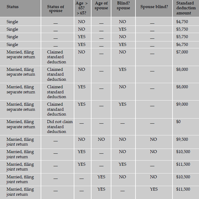
Note: Strictly speaking, the columns of a decision table should all be Boolean variables. So, we should have named the first column as “Spouse Claimed Standard Deduction?” We have used the heading “Status of Spouse” for better clarity.
The reader would have noticed that there are a number of entries marked “—” in the decision table. The values of the appropriate decision variables in these cases do not affect the outcome of the decision. For example, the status of the spouse is relevant only when the filing status is “Married, filing separate return.” Similarly, the age of spouse and whether spouse is blind or not comes into play only when the status is “Married, filing joint return.” Such entries are called don’t cares (sometimes represented by the Greek character phi, Φ). These don't cares significantly reduce the number of tests to be performed. For example, in case there were no don't cares, there would be eight cases for the status of “Single”: four with status of spouse as claimed standard deduction and four with spouse status being not claiming standard deduction. Other than this one difference, there is no material change in the status of expected result of the standard deduction amount. We leave it as an exercise for the reader to enumerate the number of rows in the decision table, should we not allow don't cares and have to explicitly specify each case. There are formal tools like Karnaugh Maps which can be used to arrive at a minimal Boolean expression that represents the various Boolean conditions in a decision table. The references given at the end of this chapter discuss these tools and techniques.
Thus, decision tables act as invaluable tools for designing black box tests to examine the behavior of the product under various logical conditions of input variables. The steps in forming a decision table are as follows.
- Identify the decision variables.
- Identify the possible values of each of the decision variables.
- Enumerate the combinations of the allowed values of each of the variables.
- Identify the cases when values assumed by a variable (or by sets of variables) are immaterial for a given combination of other input variables. Represent such variables by the don't care symbol.
- For each combination of values of decision variables (appropriately minimized with the don't care scenarios), list out the action or expected result.
- Form a table, listing in each but the last column a decision variable. In the last column, list the action item for the combination of variables in that row (including don't cares, as appropriate).
A decision table is useful when input and output data can be expressed as Boolean conditions (TRUE, FALSE, and DON't CARE).
Once a decision table is formed, each row of the table acts as the specification for one test case. Identification of the decision variables makes these test cases extensive, if not exhaustive. Pruning the table by using don't cares minimizes the number of test cases. Thus, decision tables are usually effective in arriving at test cases in scenarios which depend on the values of the decision variables.
4.4.5 Equivalence Partitioning
Equivalence partitioning is a software testing technique that involves identifying a small set of representative input values that produce as many different output conditions as possible. This reduces the number of permutations and combinations of input, output values used for testing, thereby increasing the coverage and reducing the effort involved in testing.
The set of input values that generate one single expected output is called a partition. When the behavior of the software is the same for a set of values, then the set is termed as an equivalance class or a partition. In this case, one representative sample from each partition (also called the member of the equivalance class) is picked up for testing. One sample from the partition is enough for testing as the result of picking up some more values from the set will be the same and will not yield any additional defects. Since all the values produce equal and same output they are termed as equivalance partition.
Testing by this technique involves (a) identifying all partitions for the complete set of input, output values for a product and (b) picking up one member value from each partition for testing to maximize complete coverage.
From the results obtained for a member of an equivalence class or partition, this technique extrapolates the expected results for all the values in that partition. The advantage of using this technique is that we gain good coverage with a small number of test cases. For example, if there is a defect in one value in a partition, then it can be extrapolated to all the values of that particular partition. By using this technique, redundancy of tests is minimized by not repeating the same tests for multiple values in the same partition.
Let us consider the example below, of an insurance company that has the following premium rates based on the age group.
Life Insurance Premium Rates
A life insurance company has base premium of $0.50 for all ages. Based on the age group, an additional monthly premium has to be paid that is as listed in the table below. For example, a person aged 34 has to pay a premium=base premium + additional premium=$0.50 + $1.65=$2.15.
| Age group | Additional premium |
|---|---|
| Under 35 | $1.65 |
| 35-59 | $2.87 |
| 60+ | $6.00 |
Based on the equivalence partitioning technique, the equivalence partitions that are based on age are given below:
- Below 35 years of age (valid input)
- Between 35 and 59 years of age (valid input)
- Above 60 years of age (valid input)
- Negative age (invalid input)
- Age as 0 (invalid input)
- Age as any three-digit number (valid input)
We need to pick up representative values from each of the above partitions. You may have observed that even though we have only a small table of valid values, the equivalence classes should also include samples of invalid inputs. This is required so that these invalid values do not cause unforeseen errors. You can see that the above cases include both positive and negative test input values.
The test cases for the example based on the equivalence partitions are given in Table 4.8. The equivalence partitions table has as columns:
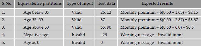
- Partition definition
- Type of input (valid / invalid)
- Representative test data for that partition
- Expected results
Each row is taken as a single test case and is executed. For example, when a person's age is 48, row number 2 test case is applied and the expected result is a monthly premium of $3.37. Similarly, in case a person's age is given as a negative value, a warning message is displayed, informing the user about the invalid input.
The above example derived the equivalence classes using ranges of values. There are a few other ways to identify equivalence classes. For example, consider the set of real numbers. One way to divide this set is by
- Prime numbers
- Composite numbers
- Numbers with decimal point
These three classes divide the set of numbers into three valid classes. In addition, to account for any input a user may give, we will have to add an invalid class—strings with alphanumeric characters. As in the previous case, we can construct an equivalence partitions table for this example as shown in Table 4.9.

Thus, like in the first example on life insurance premium, here also we have reduced a potentially infinite input data space to a finite one, without losing the effectiveness of testing. This is the power of using equivalence classes: choosing a minimal set of input values that are truly representative of the entire spectrum and uncovering a higher number of defects.
The steps to prepare an equivalence partitions table are as follows.
- Choose criteria for doing the equivalence partitioning (range, list of values, and so on)
- Identify the valid equivalence classes based on the above criteria (number of ranges allowed values, and so on)
- Select a sample data from that partition
- Write the expected result based on the requirements given
- Identify special values, if any, and include them in the table
- Check to have expected results for all the cases prepared
- If the expected result is not clear for any particular test case, mark appropriately and escalate for corrective actions. If you cannot answer a question, or find an inappropriate answer, consider whether you want to record this issue on your log and clarify with the team that arbitrates/dictates the requirements.
Equivalence partitioning is useful to minimize the numberof test cases when the input data can be divided into distinctsets, where the behavior or outcome of the product within each member of the set is the same.
4.4.6 State Based or Graph Based Testing
State or graph based testing is very useful in situations where
- The product under test is a language processor (for example, a compiler), wherein the syntax of the language automatically lends itself to a state machine or a context free grammar represented by a railroad diagram.
- Workflow modeling where, depending on the current state and appropriate combinations of input variables, specific workflows are carried out, resulting in new output and new state.
- Dataflow modeling, where the system is modeled as a set of dataflow, leading from one state to another.
In the above (2) and (3) are somewhat similar. We will give one example for (1) and one example for (2).
Consider an application that is required to validate a number according to the following simple rules.
- A number can start with an optional sign.
- The optional sign can be followed by any number of digits.
- The digits can be optionally followed by a decimal point, represented by a period.
- If there is a decimal point, then there should be two digits after the decimal.
- Any number—whether or not it has a decimal point, should be terminated by a blank.
The above rules can be represented in a state transition diagram as shown in Figure 4.3.

The state transition diagram can be converted to a state transition table (Table 4.10), which lists the current state, the inputs allowed in the current state, and for each such input, the next state.
Table 4.10 State transition table for Figure 4.3.
| Current state | Input | Next state |
|---|---|---|
1 |
Digit | 2 |
1 |
+ | 2 |
1 |
- | 2 |
2 |
Digit | 2 |
2 |
Blank | 6 |
2 |
Decimal point | 3 |
3 |
Digit | 4 |
4 |
Digit | 5 |
5 |
Blank | 6 |
The above state transition table can be used to derive test cases to test valid and invalid numbers. Valid test cases can be generated by:
- Start from the Start State (State #1 in the example).
- Choose a path that leads to the next state (for example, +/-/digit to go from State 1 to State 2).
- If you encounter an invalid input in a given state (for example, encountering an alphabetic character in State 2), generate an error condition test case.
- Repeat the process till you reach the final state (State 6 in this example).
Graph based testing methods are applicable to generate test cases for state machines such as language translators, workflows, transaction flows, and data flows.
A general outline for using state based testing methods with respect to language processors is:
- Identify the grammar for the scenario. In the above example, we have represented the diagram as a state machine. In some cases, the scenario can be a context-free grammar, which may require a more sophisticated representation of a “state diagram.”
- Design test cases corresponding to each valid state-input combination.
- Design test cases corresponding to the most common invalid combinations of state-input.
A second situation where graph based testing is useful is to represent a transaction or workflows. Consider a simple example of a leave application by an employee. A typical leave application process can be visualized as being made up of the following steps.
- The employee fills up a leave application, giving his or her employee ID, and start date and end date of leave required.
- This information then goes to an automated system which validates that the employee is eligible for the requisite number of days of leave. If not, the application is rejected; if the eligibility exists, then the control flow passes on to the next step below.
- This information goes to the employee's manager who validates that it is okay for the employee to go on leave during that time (for example, there are no critical deadlines coming up during the period of the requested leave).
- Having satisfied himself/herself with the feasibility of leave, the manager gives the final approval or rejection of the leave application.
The above flow of transactions can again be visualized as a simple state based graph as given in Figure 4.4.

In the above case, each of the states (represented by circles) is an event or a decision point while the arrows or lines between the states represent data inputs. Like in the previous example, one can start from the start state and follow the graph through various state transitions till a “final” state (represented by a unshaded circle) is reached.
A graph like the one above can also be converted to a state transititon table using the same notation and method illustrated in the previous example. Graph based testing such as in this example will be applicable when
- The application can be characterized by a set of states.
- The data values (screens, mouse clicks, and so on) that cause the transition from one state to another is well understood.
- The methods of processing within each state to process the input received is also well understood.
4.4.7 Compatibility Testing
In the above sections, we looked at several techniques to test product features and requirements. It was also mentioned that the test case result are compared with expected results to conclude whether the test is successful or not. The test case results not only depend on the product for proper functioning; they depend equally on the infrastructure for delivering functionality. When infrastructure parameters are changed, the product is expected to still behave correctly and produce the desired or expected results. The infrastructure parameters could be of hardware, software, or other components. These parameters are different for different customers. A black box testing, not considering the effects of these parameters on the test case results, will necessarily be incomplete and ineffective, as it may not truly reflect the behavior at a customer site. Hence, there is a need for compatibility testing. This testing ensures the working of the product with different infrastructure components. The techniques used for compatibility testing are explained in this section.
Testing done to ensure that the product features work consistently with different infrastructure components is called compatibility testing.
The parameters that generally affect the compatibility of the product are
- Processor (CPU) (Pentium III, Pentium IV, Xeon, SPARC, and so on) and the number of processors in the machine
- Architecture and characterstics of the machine (32 bit, 64 bit, and so on)
- Resource availability on the machine (RAM, disk space, network card)
- Equipment that the product is expected to work with (printers, modems, routers, and so on)
- Operating system (Windows, Linux, and so on and their variants) and operating system services (DNS, NIS, FTP, and so on)
- Middle-tier infrastructure components such as web server, application server, network server
- Backend components such database servers (Oracle, Sybase, and so on)
- Services that require special hardware-cum-software solutions (cluster machines, load balancing, RAID array, and so on)
- Any software used to generate product binaries (compiler, linker, and so on and their appropriate versions)
- Various technological components used to generate components (SDK, JDK, and so on and their appropriate different versions)
The above are just a few of the parameters. There are many more parameters that can affect the behavior of the product features. In the above example, we have described ten parameters. If each of the parameters can take four values, then there are forty different values to be tested. But that is not all. Not only can the individual values of the parameters affect the features, but also the permutation and combination of the parameters. Taking these combinations into consideration, the number of times a particular feature to be tested for those combinations may go to thousands or even millions. In the above assumption of ten parameters and each parameter taking on four values, the total number of combinations to be tested is 410, which is a large number and impossible to test exhaustively.
In order to arrive at practical combinations of the parameters to be tested, a compatibility matrix is created. A compatibility matrix has as its columns various parameters the combinations of which have to be tested. Each row represents a unique combination of a specific set of values of the parameters. A sample compatibility matrix for a mail application is given in Table 4.11.

The below table is only an example. It does not cover all parameters and their combinations. Some of the common techniques that are used for performing compatibility testing, using a compatibility table are
- Horizontal combination All values of parameters that can coexist with the product for executing the set test cases are grouped together as a row in the compatibility matrix. The values of parameters that can coexist generally belong to different layers/types of infrastructure pieces such as operating system, web server, and so on. Machines or environments are set up for each row and the set of product features are tested using each of these environments.
- Intelligent sampling In the horizontal combination method, each feature of the product has to be tested with each row in the compatibility matrix. This involves huge effort and time. To solve this problem, combinations of infrastructure parameters are combined with the set of features intelligently and tested. When there are problems due to any of the combinations then the test cases are executed, exploring the various permutations and combinations. The selection of intelligent samples is based on information collected on the set of dependencies of the product with the parameters. If the product results are less dependent on a set of parameters, then they are removed from the list of intelligent samples. All other parameters are combined and tested. This method significantly reduces the number of permutations and combinations for test cases.
Compatibility testing not only includes parameters that are outside the product, but also includes some parameters that are a part of the product. For example, two versions of a given version of a database may depend on a set of APIs that are part of the same database. These parameters are also an added part of the compatibility matrix and tested. The compatibility testing of a product involving parts of itself can be further classified into two types.
- Backward compatibility testing There are many versions of the same product that are available with the customers. It is important for the customers that the objects, object properties, schema, rules, reports, and so on, that are created with an older version of the product continue to work with the current version of the same product. The testing that ensures the current version of the product continues to work with the older versions of the same product is called backwad compatibility testing. The product parameters required for the backward compatibility testing are added to the compatibility matrix and are tested.
- Forward compatibility testing There are some provisions for the product to work with later versions of the product and other infrastructure components, keeping future requirements in mind. For example, IP network protocol version 6 uses 128 bit addressing scheme (IP version 4, uses only 32 bits). The data structures can now be defined to accommodate 128 bit addresses, and be tested with prototype implementation of Ipv6 protocol stack that is yet to become a completely implemented product. The features that are part of Ipv6 may not be still available to end users but this kind of implementation and testing for the future helps in avoiding drastic changes at a later point of time. Such requirements are tested as part of forward compatibily testing. Testing the product with a beta version of the operating system, early access version of the developers’ kit, and so on are examples of forward compatibility. This type of testing ensures that the risk involved in product for future requirements is minimized.
For compatibility testing and to use the techniques mentioned above, an in-depth internal knowledge of the product may not be required. Compatibility testing begins after validating the product in the basic environment. It is a type of testing that involves high degree of effort, as there are a large number of parameter combinations. Following some of the techniques mentioned above may help in performing compatibility testing more effectively.
4.4.8 User Documentation Testing
User documentation covers all the manuals, user guides, installation guides, setup guides, read me file, software release notes, and online help that are provided along with the software to help the end user to understand the software system.
User documentation testing should have two objectives.
- To check if what is stated in the document is available in the product.
- To check if what is there in the product is explained correctly in the document.
When a product is upgraded, the corresponding product documentation should also get updated as necessary to reflect any changes that may affect a user. However, this does not necessarily happen all the time. One of the factors contributing to this may be lack of sufficient coordination between the documentation group and the testing/development groups. Over a period of time, product documentation diverges from the actual behavior of the product. User documentation testing focuses on ensuring what is in the document exactly matches the product behavior, by sitting in front of the system and verifying screen by screen, transaction by transaction and report by report. In addition, user documentation testing also checks for the language aspects of the document like spell check and grammar.
User documentation is done to ensure the documentation matches the product and vice-versa.
Testing these documents attain importance due to the fact that the users will have to refer to these manuals, installation, and setup guides when they start using the software at their locations. Most often the users are not aware of the software and need hand holding until they feel comfortable. Since these documents are the first interactions the users have with the product, they tend to create lasting impressions. A badly written installation document can put off a user and bias him or her against the product, even if the product offers rich functionality.
Some of the benefits that ensue from user documentation testing are:
- User documentation testing aids in highlighting problems over looked during reviews.
- High quality user documentation ensures consistency of documentation and product, thus minimizing possible defects reported by customers. It also reduces the time taken for each support call—sometimes the best way to handle a call is to alert the customer to the relevant section of the manual. Thus the overall support cost is minimized.
- Results in less difficult support calls. When a customer faithfully follows the instructions given in a document but is unable to achieve the desired (or promised) results, it is frustrating and often this frustration shows up on the support staff. Ensuring that a product is tested to work as per the document and that it works correctly contributes to better customer satisfaction and better morale of support staff.
- New programmers and testers who join a project group can use the documentation to learn the external functionality of the product.
- Customers need less training and can proceed more quickly to advanced training and product usage if the documentation is of high quality and is consistent with the product. Thus high-quality user documentation can result in a reduction of overall training costs for user organizations.
Defects found in user documentation need to be tracked to closure like any regular software defect. In order to enable an author to close a documentation defect information about the defect/comment description, paragraph/page number reference, document version number reference, name of reviewer, name of author, reviewer's contact number, priority, and severity of the comment need to be passed to the author.
Since good user documentation aids in reducing customer support calls, it is a major contibutor to the bottomline of the organization. The effort and money spent on this effort would form a valuable investment in the long run for the organization.
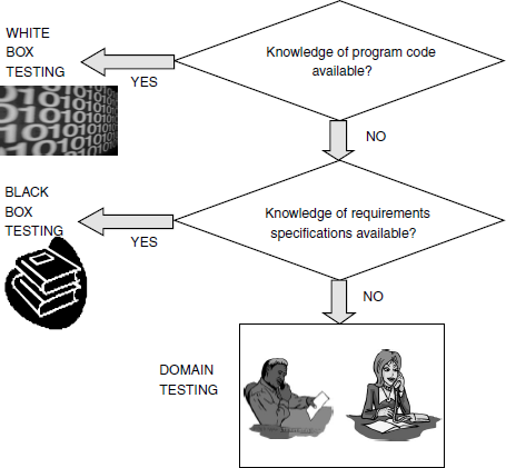
4.4.9 Domain Testing
White box testing required looking at the program code. Black box testing performed testing without looking at the program code but looking at the specifications. Domain testing can be considered as the next level of testing in which we do not look even at the specifications of a software product but are testing the product, purely based on domain knowledge and expertise in the domain of application. This testing approach requires critical understanding of the day-to-day business activities for which the software is written. This type of testing requires business domain knowledge rather than the knowledge of what the software specification contains or how the software is written. Thus domain testing can be considered as an extension of black box testing. As we move from white box testing through black box testing to domain testing (as shown in Figure 4.5) we know less and less about the details of the software product and focus more on its external behavior.
The test engineers performing this type of testing are selected because they have in-depth knowledge of the business domain. Since the depth in business domain is a prerequisite for this type of testing, sometimes it is easier to hire testers from the domain area (such as banking, insurance, and so on) and train them in software, rather than take software professionals and train them in the business domain. This reduces the effort and time required for training the testers in domain testing and also increases the effectivenes of domain testing.
For example, consider banking software. Knowing the account opening process in a bank enables a tester to test that functionality better. In this case, the bank official who deals with account opening knows the attributes of the people opening the account, the common problems faced, and the solutions in practice. To take this example further, the bank official might have encountered cases where the person opening the account might not have come with the required supporting documents or might be unable to fill up the required forms correctly. In such cases, the bank official may have to engage in a different set of activities to open the account. Though most of these may be stated in the business requirements explicitly, there will be cases that the bank official would have observed while testing the software that are not captured in the requirement specifications explicitly. Hence, when he or she tests the software, the test cases are likely to be more thorough and realistic.
Domain testing is the ability to design and execute test cases that relate to the people who will buy and use the software. It helps in understanding the problems they are trying to solve and the ways in which they are using the software to solve them. It is also characterized by how well an individual test engineer understands the operation of the system and the business processes that system is supposed to support. If a tester does not understand the system or the business processes, it would be very difficult for him or her to use, let alone test, the application without the aid of test scripts and cases.
Domain testing exploits the tester's domain knowledge to test the suitability of the product to what the users do on a typical day.
Domain testing involves testing the product, not by going through the logic built into the product. The business flow determines the steps, not the software under test. This is also called “business vertical testing.” Test cases are written based on what the users of the software do on a typical day.
Let us further understand this testing using an example of cash withdrawal functionality in an ATM, extending the earlier example on banking software. The user performs the following actions.
Step 2: Put ATM card inside.
Step 3: Enter correct PIN.
Step 4: Choose cash withdrawal.
Step 5: Enter amount.
Step 6: Take the cash.
Step 7: Exit and retrieve the card.
In the above example, a domain tester is not concerned about testing everything in the design; rather, he or she is interested in testing everything in the business flow. There are several steps in the design logic that are not necessarily tested by the above flow. For example, if you were doing other forms of black box testing, there may be tests for making sure the right denominations of currency are used. A typical black box testing approach for testing the denominations would be to ensure that the required denominations are available and that the requested amount can be dispensed with the existing denominations. However, when you are testing as an end user in domain testing, all you are concerned with is whether you got the right amount or not. (After all, no ATM gives you the flexibility of choosing the denominations.) When the test case is written for domain testing, you would find those intermediate steps missing. Just because those steps are missing does not mean they are not important. These “missing steps” (such as checking the denominations) are expected to be working before the start of domain testing.
Black box testing advocates testing those areas which matter more for a particular type or phase of testing. Techniques like equivalence partitioning and decision tables are useful in the earlier phases of black box testing and they catch certain types of defects or test conditions. Generally, domain testing is done after all components are integrated and after the product has been tested using other black box approaches (such as equivalence partitioning and boundary value analysis). Hence the focus of domain testing has to be more on the business domain to ensure that the software is written with the intelligence needed for the domain. To test the software for a particular “domain intelligence,” the tester is expected to have the intelligence and knowledge of the practical aspects of business flow. This will reflect in better and more effective test cases which examine realistic business scenarios, thus meeting the objective and purpose of domain testing.
4.5 CONCLUSION
In this chapter, we have seen several techniques for performing black box testing. These techniques are not mutually exclusive. In a typical product testing, a combination of these testing techniques will be used to maximize effectiveness. Table 4.12 summarizes the scenarios under which each of these techniques will be useful. By judiciously mixing and matching these different techniques, the overall costs of other tests done downstream, such as integration testing, system testing, and so on, can be reduced.
Performing black box testing without applying a methodology is similar to looking at the map without knowing where you are and what your destination is.
Table 4.12 Scenarios for black box testing techniques.
| When you want to test scenarios that have… | The most effective black box testing technique is likely to be… |
|---|---|
| Output values dictated by certain conditions depending upon values of input variables | Decision tables |
| Input values in ranges, with each range exhibiting a particular functionality | Boundary value analysis |
| Input values divided into classes (like ranges, list of values, and so on), with each class exhibiting a particular functionality | Equivalence partitioning |
| Checking for expected and unexpected input values | Positive and negative testing |
| Workflows, process flows, or language processors | Graph based testing |
| To ensure that requirements are tested and met properly | Requirements based testing |
| To test the domain expertise rather than product specification | Domain testing |
| To ensure that the documentation is consistent with the product | Documentation testing |
[MYER-79] and [BEIZ-90] discuss the various types of black box testing with detailed examples. [GOOD-75] is one of the early works on the use of tools like decision tables for the choice of test cases. [PRES-97] provides a comprehensive coverage of all black box testing approaches.
- Consider the lock and key example discussed in the text. We had assume that there is only one key for the lock. Assume that the lock requires two keys to be inserted in a particular order. Modify the sample requirements given in Table 4.1 to take care of this condition. Correspondingly, create the Traceability Matrix akin to what is in Table 4.2.
- In each of the following cases, identify the most appropriate black box testing technique that can be used to test the following requirements:
- “The valid values for the gender code are ‘M’ or ‘F’.”
- “The number of days of leave per year an employee is eligible is 10 for the first three years, 15 for the next two years, and 20 from then on.”
- “Each purchase order must be initially approved by the manager of the employee and the head of purchasing. Additionally, if it is a capital expense of more than $10, 000, it should also be approved by the CFO.”
- “A file name should start with an alphabetic character, can have upto 30 alphanumeric characters, optionally one period followed by upto 10 other alphanumeric characters.”
- “A person who comes to bank to open the account may not have his birth certificate in English; in this case, the officer must have the discretion to manually override the requirement of entering the birth certificate number.”
- Consider the example of deleting an element from a linked list that we considered in Problem 4 of the exercises in Chapter 3. What are the boundary value conditions for that example? Identify test data to test at and around boundary values.
- A web-based application can be deployed on the following environments:
- OS (Windows and Linux)
- Web server (IIS 5.0 and Apache)
- Database (Oracle, SQL Server)
- Browser (IE 6.0 and Firefox)
How many configurations would you have to test if you were to exhaustively test all the combinations? What criteria would you use to prune the above list?
- A product usually associated with different types of documentation — installation document (for installing the product), administration document, user guide, etc. What would be the skill sets required to test these different types of documents? Who would be best equipped to do each of these testing?
- An input value for a product code in an inventory system is expected to be present in a product master table. Identify the set of equivalence classes to test these requirements.
- In the book, we discussed examples where we partitioned the input space into multiple equivalence classes. Identify situations where the equivalence classes can be obtained by partitioning the output classes.
- Consider the date validation problem discussed in Chapter 3. Assuming you have no access to the code, derive a set of test cases using any of the techniques discussed in this chapter. Present your results in the form of a table as given below
- A sample rule for creating a table in a SQL database is given below: The statement should start with the syntax
CREATE TABLE <table name>This should be followed by an open parantehesis, a comma separated list of column identifiers. Each column identifier should have a mandatory column name, a mandatory column type (which should be one of NUMER, CHAR, and DATE) and an optional column width. In addition, the rules dictate:
- Each of the key words can be abbreviated to 3 characters or more
- The column names must be unique within a table
- The table names should not be repeated.
For the above set of requirements, draw a state graph to derive the initial test cases. Also use other techniques like appropriate to check a-c above