Chapter 1. Introducing the Ribbon User Interface

In this chapter

The Excel 2007 Interface 22

Using the Office Icon Menu 23

Understanding the Ribbon User Interface 25

Finding Old Menu Items in the New Interface 31

The Office 2007 user interface sports a complete makeover, and similar and extensive changes have been made to Excel, Word, PowerPoint, Access, and the Compose Mail portion of Outlook. With the new interface, Microsoft admits that it was wrong when it used the original menu and toolbars paradigm back in 1985. Microsoft admits that it was wrong to try adaptive menus in 2000. It admits that the task pane was wrong in Excel 2003. It admits that Clippy (the much-maligned Office Assistant) was the stupidest idea ever invented. Even if everyone agrees that these were bad ideas, it is shocking to have them taken away. (Except Clippy. I don’t think anyone will miss Clippy). They may have been bad ideas, but we became familiar with them. Next week, when you are under pressure to close the books for the month, you will really wish those horrible menu items were back so you could get your work done.

I did not write this chapter first. I wanted to let the new Ribbon interface sink in for a while. I wanted to give it a chance. I can report, after several months of using Excel 2007, that I understand the Ribbon interface. I can almost always go directly to the correct ribbon. A few things are definitely easier with the Ribbon interface. My goal in this chapter is to give you a quick start to help you quickly get used to the Ribbon interface.

The Excel 2007 Interface

Figure 1.1 shows the new Excel 2007 window. Note that the new interface has the following elements:

Figure 1.1. The Excel 2007 interface includes several new elements.

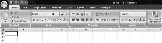
• The Office icon menu—This menu contains most items that used to be on the File menu. In the original beta versions of Excel, the Office icon menu was even called the File menu.
• The Quick Access toolbar—The Quick Access toolbar can be customized to include your favorite command icons. See Chapter 2 for information on customizing the Quick Access toolbar.
• Tabs for Home, Insert, Page Layout, and other ribbons—Each tab leads to a different ribbon. Figure 1.1 shows the Home ribbon.
• Groups—Each ribbon is divided into related commands. The name of each group appears at the bottom of the ribbon. In Figure 1.1, the groups shown are Clipboard, Font, Alignment, and Number. While you never specifically have to click on these names, they can assist you in finding a command on a busy ribbon. This book refers to them when directing you to a command.
• Drop-down buttons—With some buttons on the ribbon, a button for the most popular choice is attached to a drop-down icon. For example, the Paste icon on the left side of the Home ribbon is such a button. You can click the top half of the icon to initiate a paste, or you can click the drop-down arrow to display a menu of paste-related commands.
• Dialog launchers—You can click this icon in the lower-right corner of some groups to return to the familiar legacy version of the dialog box for that function.

The following sections describe the various components of the Excel 2007 interface.

Using the Office Icon Menu

The Office icon in the upper-left corner of the screen contains menu options for saving, printing, and sharing with others. You can click the Office icon to display its menu, as shown in Figure 1.2.

Figure 1.2. The Office icon menu includes many items from the old File menu.

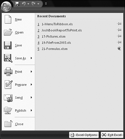
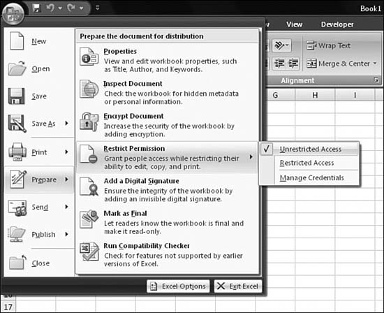
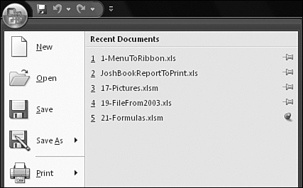
The Office icon menu contains menu items such as Save and Close that are straightforward choices. If you click one of those menu items, a command is performed. Other menu items, such as New, Open, and Print lead to dialog boxes where you can specify details about the command. With some commands, there is a right arrow next to the command. You can hover your mouse over this arrow to display a fly-out menu with more options, as shown in Figure 1.3.

Figure 1.3. Some menu items lead to fly-out menus reminiscent of prior versions of Excel.

Customizing the Recent Documents List

In prior versions of Excel, anywhere from four to nine of your recently used files would appear at the bottom of the File menu. This feature has been greatly improved and expanded in Excel 2007. You can now choose to display up to 50 recent documents. To change the limit, you choose the Office icon, Excel Options, Advanced, Display. Then you use the Show This Number Of Recent Documents spin button to increase the number to up to 50.

The Recent Documents list is more thorough in Excel 2007 than in previous versions. If you open a workbook by double-clicking the file in Windows Explorer, the workbook is logged to the Recent Documents list. This is an improvement over Excel 2003, where the recently used file list would routinely skip files that were not opened through the Excel File menu.

As shown in Figure 1.4, there is a gray thumbtack to the right of each file in the list. If you click the thumbtack, you pin that file to the list. Files that are pinned to the list appear in the Recent Documents list until you unpin them. To unpin an item, you click the thumbtack icon again. In the figure, the last file is pinned to the list.

Figure 1.4. Files can be pinned to permanently appear in the Recent Documents list.

Using the Excel Options and Exit Excel Buttons

You can click the Exit Excel button to close Excel. When you do, Excel prompts you to save any unsaved documents.

Clicking the Excel Options button opens the Excel Options dialog, which allows you to set more than 100 settings in several categories. You can use this dialog to access Office Online, activate your installation of Office, and customize the Quick Access toolbar. (For details on customizing the Quick Access toolbar, see Chapter 2, “The Quick Access Toolbar.” For details on the Excel Options dialog, see Chapter 6, “The Excel Options Dialog.”)

Understanding the Ribbon User Interface

The Ribbon user interface is the area at the top of the Excel window that contains all the features of the program. The Ribbon user interface is organized into a number of ribbons, such as Home, Insert, and Page Layout, that group features together.

Every ribbon is static. Items are not added to or removed from a ribbon in response to your actions in Excel. Unlike the adaptive menus introduced in Excel 2000, every person’s Formulas ribbon looks identical to every other person’s Formulas ribbon all the time (assuming that they have not been altered by a programmer, as described shortly).

It is possible for entire context-sensitive tabs to appear and disappear. For instance, the Picture Tools ribbon is visible only when there is a picture on your worksheet and the picture is selected. If you aren’t working with the picture, the tab for Picture Tools is put away.

Minimizing the Ribbon

If you are working on a tablet PC or a laptop with a small screen, you might find that the Ribbon takes up too much space on your screen. You can choose to minimize the Ribbon. In this state, you will see only the Office icon, the Quick Access toolbar, and the ribbon tab names.

When the ribbon is minimized, you can click on a tab name and Excel will temporarily open that particular ribbon. After you have selected a command, the ribbon will automatically return to the minimized state.

To toggle into or out of having the Ribbon minimized, use one of these methods:

• Press Ctrl+F1
• Right-click the Ribbon and choose “Minimize the Ribbon”

Changing the Ribbon

The ribbons are always at the top of the screen. You cannot undock the ribbons and move them to a new location.

A programmer using XML can add new groups to an existing ribbon tab or can add new ribbon tabs. This is a disappointing change from the past 15 years of Excel. In any prior version, any person who could right-click and drag could customize a toolbar, create a new toolbar, or undock a toolbar so it could float in the work area. (All the Office MVP were vocal in their criticism of Microsoft for this decision.)

The bottom line is that if Microsoft allowed for customization of toolbars, anyone could basically design a toolbar to look like the old version of Excel. Because Microsoft is betting the ranch on the new user interface, it wants you to live with it and experience it. As Microsoft sees it, allowing you to go back to the way that you knew and loved would be counterproductive.

The ribbon tabs often expand to fill the space available depending on the resolution of your display. If you start to shrink the application, Excel replaces the large icons with smaller icons but keeps the groups in their original order.

Although there are initially 7 ribbon tabs available, there are a total of 26 ribbon tabs in Excel 2007. The following sections describe the ribbons you are most likely to use.

Using the Common Commands on the Home Ribbon

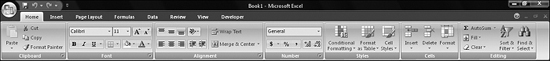
Microsoft put the most common features on the Home ribbon. This ribbon includes cut, copy, and paste functions. Font formatting, cell alignment, and number formatting also appear on the Home ribbon. The new conditional formatting features have been placed to the Home ribbon, as have features related to tables, formatting, and editing.

Figure 1.5 shows the Home ribbon.

Figure 1.5. The most common commands are on the Home ribbon.

Using the Eclectic Commands on the Insert Ribbon

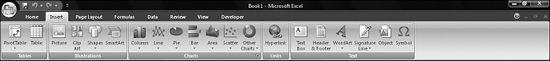
The Insert ribbon is the gateway to the fantastic new charting engine, with seven large icons dedicated to various chart types. You can also use this ribbon to insert shapes, pivot tables, illustrations, hyperlinks, and various text objects.

Figure 1.6 shows the Insert ribbon.

Figure 1.6. Charting and pivot tables are found on the Insert ribbon.

Controlling Themes and Page Setup with the Page Layout Ribbon

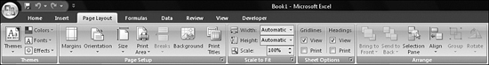
Almost everything that used to be on the four-tab Page Setup dialog is now spread out across the Page Layout ribbon. The Scale to Fit options finally make sense after 15 years of being confusing.

Document themes, which are new to Excel 2007, allow you to quickly change a document to any of 20 built-in themes or custom themes that you design to match your corporate or some other color scheme. Word, PowerPoint, and Excel all offer the same 20 built-in themes, so all your Office creations can feature a consistent color scheme.

The Page Layout ribbon also includes custom views and various options for arranging objects on the worksheet (see Figure 1.7).

Figure 1.7. Most of the information from the old Page Setup dialog is now on Page Layout ribbon.

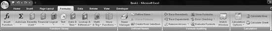
Calculating with the Formulas Ribbon

Excel 2007 introduces the AutoComplete feature, which you can use when building formulas in Excel. You begin building formulas graphically by using the function library icons on the Formulas ribbon. The improved Name Manager and other cell naming tools are in this ribbon.

If you frequently build complex formulas, you will love the Evaluate Formula and Watch Window options in the Formulas ribbon. Both features were added to Excel 2003, but they were so buried that most people never found them.

Finally, calculation options have been promoted from the Options dialog to a spot at the end of the Formulas ribbon, as shown in Figure 1.8.

Figure 1.8. You can build and audit formulas by using the Formulas ribbon.

Managing Data Connections with the Data Ribbon

With the introduction of Excel Services for SharePoint, Microsoft realizes that Excel is often the presentation layer for data stored in corporate systems. Connections to external data, whether in Access, on the Web, or from SQL Server, can be managed from the Data ribbon, as shown in Figure 1.9.

Figure 1.9. You can manage external data connections by using the Data ribbon.

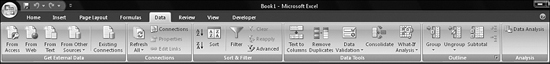
Several of the icons for sorting and filtering that appear in drop-downs on the Home ribbon are repeated on the Data ribbon. The gem on this ribbon is the Subtotals command. If you regularly have to insert totals after each customer or region, you should read Adding Automatic Subtotals in Chapter 35, “More Tips and Tricks for Excel 2007.”

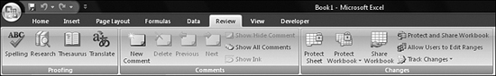
Reviewing Documents with the Review Ribbon

All the reviewing tools, such as spellcheck, the thesaurus, and the new translation feature are on the Review ribbon, as shown in Figure 1.10. This ribbon also includes comment features from the old Reviewing toolbar, as well as protection and sharing options. The translation service is discussed in Chapter 35.

Figure 1.10. Spellcheck and thesaurus tools are on the Review ribbon.

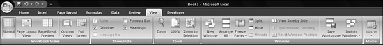
Seeing More with the View Ribbon

The Window menu was one of my most frequently visited menus in Excel 2003. Most of its options are now on the View ribbon in Excel 2007.

The new Page Layout view is a terrific addition to Excel 2007. Strangely, though, you can switch to this view by using the buttons near the right edge of the status bar. The large icons Normal, Page Break Preview, and Zoom are all duplicated and always visible in the status bar.

The icons in the Window group allow you to freeze titles at the top or left of the worksheet or switch to a different open workbook.

One feature available on the View ribbon is View Side by Side. If you have two workbooks open, you can scroll them simultaneously by using this feature that was introduced in Excel 2003. An old but often-overlooked feature allows you to see two worksheets from the same workbook simultaneously. To take advantage of this feature, you select New Window and then Arrange.

Figure 1.11 shows the View ribbon.

Figure 1.11. The old Window menu options are now on the View ribbon.

Managing Macros with the Developer Ribbon

There is a ribbon just for those who regularly write VBA macros. Excel initially hides the Developer ribbon, but you can follow these steps to display it:

1. Click the Office icon menu.
2. Select Excel Options.
3. Select the Popular category.
4. In the Top Options For Working with Excel section, choose Show Developer Tab in the Ribbon.
5. Click OK.

As shown in Figure 1.12, the Developer ribbon offers one-click access to the Visual Basic Editor. The Macros button lists the available macros in the current workbook (similar to pressing Alt+F8 in Excel 2003).

Figure 1.12. Macro programmers will want to enable the Developer ribbon.

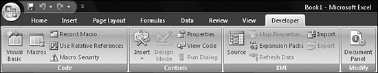
Other options in the Developer tab include XML settings and the options from the old Control toolbox, which are now located under Controls, Insert.

Accessing the Context-Sensitive Ribbons

Excel 2007 has 18 additional ribbons that appear as necessary. All these ribbons are context sensitive. If you edit a page header in your worksheet, the Header & Footer Tools ribbon appears. When you click outside of the header, the Header & Footer Tools ribbon is put away.

Sometimes, there are more items than can fit on a single ribbon. For example, Chart Tools offers three ribbons: Design, Layout, and Format. In general, if a context menu includes multiple ribbons, the general options appear on the leftmost ribbon. The more specific items appear on additional ribbons to the right.

These are the context-sensitive ribbons:

• Add-Ins—This ribbon contains any menu items added through VBA macros or add-ins.
• Chart Tools—The Chart Tools ribbon includes three ribbons: Design, Layout, and Format. The Design ribbon provides features to change an entire chart. By the time you get to the Format ribbon, you are micromanaging small aspects of a chart.
• Drawing Tools—This ribbon includes a Format ribbon for working with shapes. To access the ribbon, you select Insert, Shapes.
• Header & Footer—This ribbon appears when you are editing the header or footer for a page in Page Layout view. To access the ribbon, you click View, Page Layout View and then click in either the header or footer zone.
• Ink Tools—This ribbon is for tablet PCs.
• Picture Tools—This ribbon is available after you insert clip art or an image and select the illustration.
• Pivot Chart Tools—After you insert a pivot chart, four new ribbons are available: Design, Layout, Format, and Analyze. The first three of these ribbons are similar to the ribbons on the Chart Tools ribbon. The fourth contains the pivot table features.
• Pivot Table Tools—This ribbon includes two ribbons: Options and Design. The major settings appear on the Options ribbon. Formatting options appear on the Design ribbon.
• Print Preview Tools—This small ribbon appears as the only ribbon when you are in Print Preview mode.
• SmartArt Tools—In Excel 2007, the former business diagrams has been renamed SmartArt. When you are working with organization charts or other SmartArt diagrams, two new ribbons are available: Design and Format.
• Table Tools—The Design ribbon allows for the formatting of a database in Excel after it has been converted to a table. In Excel 2007, tables replace Excel 2003 lists.

All these context ribbons come and go as you select and unselect certain items in Excel.

Finding Old Menu Items in the New Interface

For the first few weeks that you use Excel, you will probably often try to figure out exactly where Microsoft decided to move a command. Table 1.1 shows each of the menu items in Excel 2003, followed by the current location of each command in Excel 2007.

Table 1.1. Excel 2003 Menu Items and Their Locations in Excel 2007

Sometimes, a command is no longer offered in the Ribbon User Interface, but the icon is still available for you to add to the Quick Access toolbar. For these commands, the second column will say, “Office Icon, Excel Options (Add to Quick Access toolbar if you need it).” See Chapter 2 for information about customizing this toolbar.

In other cases, a command is no longer available in Excel 2007. In these cases, the second column will say, “(no equivalent).”

Table 1.2 shows all the icons in the default Standard toolbar in Excel 2003, along with their equivalent locations in Excel 2007.

Table 1.2. Excel 2003 Standard Toolbar Icons and Their Excel 2007 Equivalents

Table 1.3 shows the standard Formatting toolbar icons in Excel 2003, along with the locations of the equivalent commands in Excel 2007.

Table 1.3. Excel 2003 Formatting Toolbar Icons and Their Excel 2007 Equivalents