CHAPTER 5

INVESTMENT PRINCIPLES

Speculating is not investing

It is easy to confuse speculating with investing. Speculating is trying to second-guess what investment markets will do with the intention of exploiting those expected movements for financial gain. Speculating is win–lose in that if you make the right choice you win and if you make the wrong one you lose. Investing is not win–lose because capitalism will provide a return on your capital over the long term. You lose only if your belief in capitalism fails or capitalism itself collapses. Most retail investment advice is actually speculating advice. While speculating might be exciting, the available evidence suggests that it is like all gambling and is seriously bad for your wealth. History is full of examples of wealth destroyed by those two powerful human emotions of greed and fear.

Speculation is what fuels an investment ‘bubble’, whether that is equities, property, gold or tulips bulbs. As more and more people see the easy money that others are making, they start speculating until eventually the whole thing collapses, as is well illustrated by Figure 5.2. The sad thing about bubbles is that in seeking abnormal investment returns, speculators miss out on the meaningful and worthwhile reasonable investment returns there for the taking.

Figure 5.2 Main stages in a bubble

Source: Reproduced by kind permission of Dr Jean-Paul Rodrigue, Department of Global Studies and Geography, Hofstra University.

Capitalism and markets do work

For all its faults and shortcomings, the capitalist system is the only economic system that has actually stood the test of time. Capital and resources (both human and physical) are the two essential ingredients for economic activity, which arise directly from the human race’s desire to maintain and improve its standard of living (see Figure 5.3). In a perfect world all capital and resources would be used in the most efficient manner and the maximum return would be achieved for the minimum effort. However, we don’t live in a perfect world and, as such, capital and resources are not always allocated efficiently. This does not mean that the capitalist model is wrong, just that it is imperfect.

Figure 5.3 Capitalism creates wealth

Over the past few decades we have seen major changes in the world economic order and this came to a head with the recent global financial crisis. There is no doubt that many things went seriously wrong with regulation, product innovation and world economic policy, but that is not to say that capital markets failed. In proper open capital and labour markets, with no political interference and rigorous and credible pricing and clearing/settlement mechanisms, returns would be properly allocated in the most efficient way.

The accumulated empirical evidence, research and theory suggest we should trust in capitalism as this is the only system that creates wealth and allocates capital effectively enough over the long term, as illustrated in Figure 5.4. In addition, capital markets are generally efficient and provide an effective equilibrium (self-levelling) system in terms of setting the price of securities. The aggregate current market view is the best gauge of the value of an investment and represents the value of expected future dividends and earnings for companies and interest payments for fixed-income investments.

Risk and return are linked

Risk and return go hand in hand and if you want higher returns you have to take higher risks. There are no shortcuts and if an investment offers more than the risk-free rate (generally defined as very short-term government deposits) then it comes with higher risks, in terms of capital loss and the possibility that the investment return will turn out to be lower than anticipated. Diversification means allocating your capital across different asset classes (not having all your eggs in one basket) and it can help reduce the various risks associated with investing. In this regard diversification can be viewed as just about the only ‘free lunch’ available in investing, in that no one else has to lose to enable you to benefit.

Figure 5.4 Monthly growth of wealth (£) 1956–2013

Source: Data from Dimensional Fund Advisors, FTSE, Office for National Statistics, London Business School; Bloomberg securities, StyleResearch, London Share Price Database.

The next step is to identify the various investment risks and how they are compensated, then decide whether (or not) to take them. Once you have decided on how much exposure you will have to the various risk factors, you (or your adviser) need to manage that exposure closely to ensure that it doesn’t increase over time.

Equity risk

William Sharpe shared the Nobel Prize in Economics in 1990 for his pioneering contribution to asset pricing theory. He developed the Capital Asset Pricing Model (CAPM) to try to explain, using simplifying assumptions, that an equity’s expected return is a function of its volatility (price movements) relative to the volatility of the universe of risky assets. The expected higher returns from equities come with associated risks. These risks are a combination of ‘systematic’ and ‘unsystematic’ risk.

• Systematic risk includes macroeconomic conditions affecting all companies in the stock market. Systematic risk cannot be diversified away.
• Unsystematic risk includes company risk (the specific risk of owning shares in, for example, Barclays, GlaxoSmithKline or Rolls-Royce) and industry risk (such as pharmaceutical, banking or telecom shares) specific to individual securities. The effect of these can be reduced through sufficient diversification (i.e. allocating capital across a number of different securities, sectors and markets).

Sharpe’s conclusion was that the most efficient portfolio, from a risk–return perspective, is one containing the entire universe of risky assets. The CAPM model is the intellectual foundation of the total stock market index fund. The lesson for investors is that they should not expect markets to reward them for risks that can be diversified away. Rather, they should expect compensation only for bearing systematic risks. Figure 5.5 illustrates this concept visually.

Figure 5.5 Total equity risk

The multi-factor model

Sharpe’s CAPM model was developed further in the early 1990s by two eminent US finance academics, Professors Eugene Fama and Kenneth French. They developed a framework, known as the multi-factor model, for explaining two more systematic risk factors relating to equity investment.³ Fama and French found that 96% of the variation in returns among equity portfolios can be explained by the portfolios’ relative exposure to three compensated risk factors:

1. Market factor – equities have higher expected returns than fixed-income securities.
2. Size factor – small capitalisation (i.e. smaller companies’) equities have higher expected returns than large capitalisation (i.e. larger companies’) equities.
3. Value factor⁴ – lower-priced (relative to their accounting value) ‘value’ equities have higher expected returns than higher-priced ‘growth’ equities.

The market factor

The first factor in the model relates to how much of a portfolio is allocated to the stock market, i.e. equities, which is defined as the complete universe of companies on a market value-weighted basis. Because equities have a higher risk than fixed interest investments and cash deposits, they have to have a higher expected return, otherwise no rational investor would be willing to own them. This higher expected return is known as the equity risk premium (ERP).

The ERP is not a static figure and will rise and fall with changes in economic conditions and the supply of and demand for capital by companies. Intuitively we know that an ERP must exist, otherwise investors would invest solely in less risky investments like cash and bonds. There is no definitive or universally accepted way of measuring the equity risk premium, but it is reasonable to say that the long-term ERP has a floor of around 0.50–1% p.a., this being the real yield on index-linked gilts.

Historical analysis of the UK, US and global (in US$ terms) equity markets’ ERPs to the end of 2013 was 3.9%, 4.5% and 3.3% respectively.⁵ Some academics expect the ERP for global developed equity markets in the next ten years or so to be lower, about 3–3.5%, whereas others think that it will be about 4%, which is in line with its long-term historic average.⁶ Figure 5.6 shows the historic and forward-looking estimates for the ERP. While the historic ERP is almost certainly unlikely to be repeated, no one has devised a reliable method of forecasting what it might be in the future. It is precisely because there is so much uncertainty about the ERP that investors need to regularly review their investment strategy and spending levels in the light of actual returns achieved.

Figure 5.6 The equity risk premium in developed markets

Sources: Data from Dimson, E., Marsh, P. and Staunton, M. (2014) Credit Suisse Global Investment Returns Yearbook 2014; Hammond, P.B. Jr and Leibowitz, M.L. (2011) Rethinking the equity risk premium: An overview and some new ideas’, Research Foundation of CFA Institute, December, pp. 1–17; Dimson, E., Marsh, P. and Staunton, M. (2006) ‘The worldwide equity premium: A smaller puzzle’, 7 April, EFA 2006 Zurich Meetings Paper; JP Morgan Asset Management (2013) ‘Long-term capital market assumptions 2014’, 30 September.
Source: Historical ERP – footnote 5 (above); Academic consensus ERP – footnote 6; DMS estimate – footnote 9; JP Morgan estimate – footnote.⁷ Note* – top end of 3.0% to 3.5% estimate.

Jack Bogle, the founder of index fund provider Vanguard, suggests a simple way to determine the future return from equities.⁸ If the dividend yield is 2–3% and long-term real growth in earnings is 2–3%, the real return from equities would need to be in the region of 5%, which is a 4% premium over T-bills (a cash-like government security), assuming no change in the price/earnings ratio. This seems a reasonable assumption for the basis of financial planning decisions, providing that regular reviews of the financial plan and investment strategy are carried out.

‘The main message is that the unconditional expected [i.e. future] equity premium … is probably far below the realised [historical] premium.’⁹

There are periods when investors in equities experience extreme negative real returns. As illustrated in Figure 5.7, over 20 years or more even the worst returns from UK equities since 1899 have still generated positive purchasing power growth, but that isn’t to say this will necessarily be repeated in the future. Uncertainty is the price you have to pay to capture the higher expected returns from equities compared with cash and bonds (see Figure 5.8).

Figure 5.7 Historic equity return variations

Source: Barclays Equity Gilt Study 2014.

The size factor

The second risk factor that Fama and French identified as impacting on returns is the size of the company. Smaller companies have lower capitalisation than larger ones and tend to be more vulnerable to adverse trading conditions. As such, even if such companies have high growth prospects, they are more risky than big companies and therefore have to pay more for their capital. This higher cost of capital for the company translates into additional potential return for the investor. The smaller companies’ premium (the additional return) fluctuates all the time and sometimes larger companies outperform (see Figure 5.9). However, Fama and French’s multi-factor research indicates that there is a greater probability of higher long-term returns from smaller companies to compensate investors for these additional risks. While some experts reject the notion of the size factor, and it is certainly less compelling than other factors, it does stand up to academic scrutiny.

Figure 5.8 Equities versus cash over the past 57 years to 31 December 2012

Source: Data on UK one-month T-bills provided by Datastream; prior to January 1975, UK three-month T-bills. UK market is the FTSE All-Share Index. FTSE data published with the permission of FTSE.

Figure 5.9 Smaller companies premium – UK small versus UK market to 31 December 2012

Source: UK small data simulated from StyleResearch securities data; prior to July 1981, Hoare Govett Smaller Companies Index, provided by the London School of Business. UK market is the FTSE All-Share Index. FTSE data published with the permission of FTSE.

The value factor

The third factor that Fama and French identified was the value factor. Some companies are viewed by the market as ‘unhealthy’ and this can arise for a number of reasons, such as having poor growth prospects, being involved in a risky trading activity or having suffered continued falls in profitability. As a result, these companies have to pay more for their capital to compensate investors for the additional risk to their capital, which translates into the investor’s additional potential return over that available from the main equity market. These financially unhealthy companies are known as ‘value’ companies because they have what is known as a high book (balance sheet) to market (share price) ratio. Put another way, the share price is low compared with the net assets of the company.

Some of the few successful active fund managers, those who have achieved significant outperformance of the stock market, have actually been value company investors. However, once the risk factors associated with value companies are stripped out, we can determine that in most cases the investment manager’s skill actually had little influence on the outperformance. Just as the equity risk premium fluctuates all the time, so does the value premium. There have been periods when growth companies (those that the market views as healthy and less risky) have outperformed value companies. However, the research suggests that the value premium does exist across multiple markets and has a higher probability of being delivered over long time periods (see Figure 5.10).

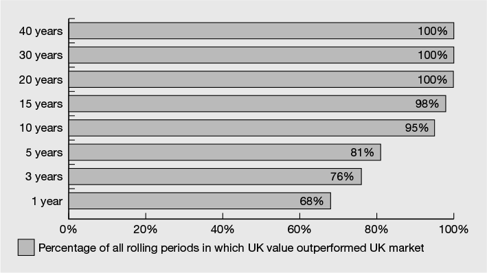
Figure 5.10 The value premium – UK value versus UK market to December 2012

Source: Data from UK market is the FTSE All-Share Index. FTSE data published with the permission of FTSE. UK value simulated Bloomberg securities data; prior to 1994, data provided by London Business School.

Various research papers have confirmed that the small companies’ and value companies’ risk premia exist in both overseas developed and emerging markets and are of the same quantum as for UK markets (see Figure 5.11).

Figure 5.11 Size and value effects across global equity markets to December 2012

Source: US value and growth index data (ex utilities) provided by Fama/French. FTSE data published with the permission of FTSE. The S&P data are provided by Standard & Poor’s Index Services Group. CRSP data provided by the Center for Research in Security Prices, University of Chicago. MSCI Europe Index is gross of foreign withholding taxes on dividends; copyright MSCI 2013, all rights reserved. Emerging markets index data simulated by Fama/French from countries in the IFC Investable Universe. Value stocks are above the 30th percentile in book-to-market ratio. Growth stocks are below the 70th percentile in book-to-market ratio. Simulations are free-float weighted both within each country and across all countries. UK and Europe data provided by London Business School/StyleResearch.

The multi-factor model therefore helps us to decide how to allocate a portfolio to the different asset classes based on risk and expected returns. It also supports the contention that making further distinctions between different sectors such as industrials and mining is unlikely to add much value because they are merely components of equities as an asset class and don’t have sufficiently different risk and return attributes from equities as a whole. In the same way, geographical distinctions in overseas developed or emerging markets are probably less important than one might expect because it is the risk of the asset class as a whole that is the main determinant of returns.

Taken together, the three main equity risk factors of market, size and value account for around 96% of the variation in returns between portfolios. Using a multi-factor approach, you have the potential to earn higher expected returns by increasing exposure to compensated risk factors rather than trying to market time either your asset allocation or the underlying equity or bond holdings (see Figure 5.12).

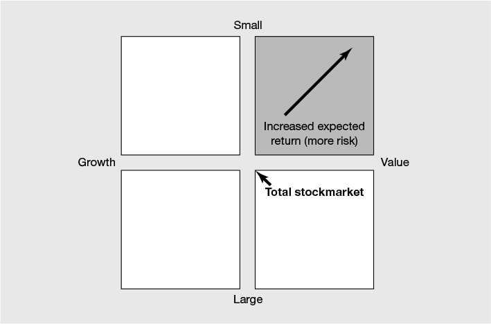
Figure 5.12 Risk factor exposures

Expected profitability

A relatively new investment factor – expected profitability – has emerged over the past decade.¹⁰ Researchers have observed that certain highly profitable companies, which have a statistically higher probability of maintaining those profits, tend to have higher returns than the stock market as a whole.¹¹ All other things being equal, if two companies have the same expected profitability ratio then it makes sense to buy the cheaper of the two. Similarly, if two companies have the same share price, it makes sense to buy the one with the highest expected profitability ratio. Some experts are of the opinion that expected profitability is not a new factor but merely another way of assessing value-type companies that under-invest and achieve higher profitability for a period of time. Whether or not they are correct, some innovative investment managers are starting to incorporate expected profitability into their trading strategies, as a means of enhancing returns from this factor.

‘It has always been about the price, and it still is. If two firms have the same number of shares outstanding, we buy the one with the lower price. If two firms have the same book value, we buy the one with the lower price. If two firms have the same profitability, we buy the one with the lower price. It just makes sense.’

David Booth, Co-CEO Dimensional Fund Advisors¹²

Bond maturity and default premium

The real return from government bonds (fixed interest securities issued to fund government debt) has averaged about 2.5% p.a. compounded over the past 50 years.¹³ Bonds with a longer time until they mature usually pay a higher return than cash or bonds with a shorter time until maturity. Although not identified by them, Fama and French’s multi-factor research also referred to two other factors that related to bonds: maturity date and credit quality (the credit rating of the organisation issuing the bond). (See Figure 5.13.)

Bonds issued by companies and governments that are perceived to be more risky, as they may not meet some or all of the bond interest payments or repay the capital on maturity, pay a higher return than those from less risky issuers. However, if the role of fixed income is to lower the risk of a portfolio, then if you invest in longer-term bonds and/or those with a lower credit quality you are unlikely to be sufficiently compensated for the risks taken. We’ll go into more detail about bonds in Chapter 6.

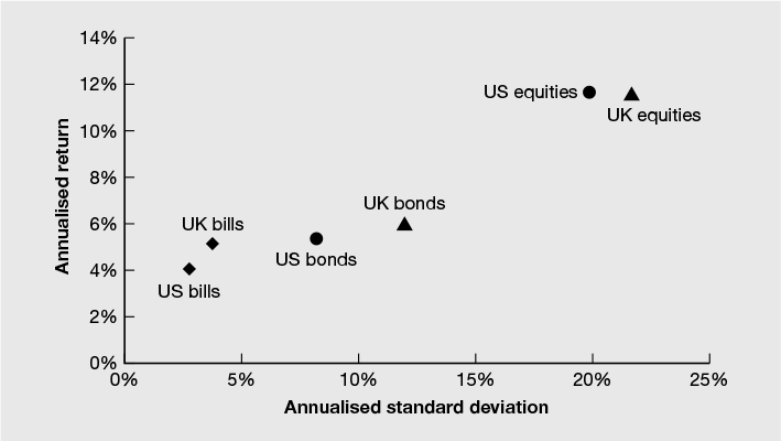
Figure 5.13 Risk and return of UK and US bonds, 1900–2000

Source: Data from Dimson, E., Marsh, P. and Staunton, M. (2001) Millennium Book II: 101 years of investment returns, ABN AMRO and London Business School. This publication defines the data used for the above chart and matrix as follows: UK bills are UK one-month Treasury bills (FTSE). UK bonds are the ABN AMRO Bond Index. UK equities are the ABN AMRO/LBS Equity Index. US bills are commercial bills 1900–1918 and one-month US Treasury bills (Ibbotson) 1919–2000. US bonds are government bonds 1900–1918, the Federal Reserve Bond Index 10–15 Years 1919–1925, Long-Term Government Bonds (Ibbotson) 1926–1998, and the JP Morgan US Government Bond Index 1999–2000. US equities are Schwert’s Index Series 1900–1925, CRSP 1–10 Deciles Index 1926–1970, and the Dow Jones Wilshire 5000 Index 1971–2000.

Focus on the mix of assets

‘Let every man divide his money into three parts, and invest a third in land, a third in business, and a third let him keep in reserve.’

Talmud, c. 1200 BC–AD 500

Asset allocation is the process of dividing up your capital and allocating it to one or more different types of asset classes. An asset class is the term given to a group of investments that share similar risk and return characteristics – examples include cash, equities, fixed interest, property and commodities. In addition, there are a number of investment types known as ‘alternative’ asset classes, because they fall outside the mainstream asset classes (although, confusingly, some regard property and commodities as ‘alternatives’). Table 5.1 shows the main investment characteristics of the three key asset classes – cash, fixed interest and equities – that are the main building blocks used in most portfolios.

Table 5.1 Characteristics of the main asset classes

Because asset allocation is the principal determinant in the variation in returns in a broadly diversified portfolio,¹⁴ it is critical to get the right strategic asset mix in place at the outset and to maintain that mix. At the high level you need to determine the overall split between growth (equity-type) and defensive (bond-type) assets. Think of growth as whisky and defensive as water. If you like a strong drink you may not add any water, but be prepared for a big kick. If you don’t like alcohol or can’t hold your drink then water will probably be all you need. The same goes for investing, in that you need to determine the right blend of assets, taking into account the return that you need and the risks with which you can cope. Equities are expected to generate higher returns than cash or bonds over the long term. This makes sense as equity owners are taking the highest level of risk of these three asset classes.

Income-type assets provide most if not all the return in the form of income. Income investments include cash, bonds and certain equities. Returns tend to be more stable but lower over the long term and are more vulnerable to the effects of inflation. Growth-type investments provide most of the return in the form of capital growth over time. Examples of growth investments include most types of global and emerging market equities. Growth investments have the potential to produce higher real returns than defensive asset classes over the long term, but usually pay low or no dividends. However, this usually translates into them having much more volatile returns, due to more frequent trading and changes in investor sentiment. Figure 5.14 sets out a graphical asset allocation decision framework to help you to understand the three stages and the components of each stage.

Figure 5.14 Asset allocation decision framework

Measuring investment risk

Investment risk can take various forms, including currency risk, inflation risk, interest rate risk and credit risk. However, a widely used measure of risk relates to how investment returns vary from the long-term average, otherwise referred to as the volatility of investment returns; therefore, the term volatility may be used interchangeably with risk.

Standard deviation is a means of measuring volatility over a series of time periods.¹⁵ As illustrated in Figure 5.15, the higher the standard deviation figure, the more the returns have varied from the average. As a general rule, higher average returns usually come with a higher standard deviation (as risk and return are related); such investments can and do experience big swings in returns above and below the average.

The magnitude and likelihood of the return varying from the average is expressed as a multiple of the standard deviation number. Assuming that the data set is large enough to be representative, a particular period’s return will fall within one standard deviation either side of the average about 65% of the time, while it will fall within two standard deviations about 95% of the time and within three standard deviations about 99% of the time.

Figure 5.15 Standard deviation

To help you to understand standard deviation, consider the following two investments set out in Table 5.2. Investment X has a lower average annual return (3%) than investment Y (8%), but it also has a much lower range of higher and lower annual returns. So, 65% of the time (one standard deviation) we can see that investment X delivered a return as low as 2% (3% – 1%) and as high as 4% (3% + 1%). By comparison, investment Y delivered a return as low as –7% (8% – 15%) and as high as 23% (8% + 15%).

Table 5.2 Investment returns and risk

However, if we want to include a wider range of outcomes, we need to look at the range of returns that falls within 95% of the investment period (two standard deviations). In this instance, we can see that investment X delivered as low as 1% (3% – 2%) and as high as 5% (3% + 2%) in 95% of the investment period. Investment Y, meanwhile, delivered as low as –22% (8% – 30%) and as high as 38% (8% + 30%) in 95% of the investment period.

Think of standard deviation like temperature. The long-term average temperature for the UK in July might be 20°C, but there is a possibility that it might be as high as 30°C and as low as 10°C, although it is highly unlikely ever to go below 0°C. Perhaps in October the long-term average might be 10°C, but it could be as high as 22°C and as low as –2°C (a standard deviation of 12°), thus it could go below zero.

Standard deviation is a statistical measure that can be used in a wide variety of applications not limited to financial planning. It is therefore important not to imbue it with magical predictive value as it is entirely dependent on the data set used to calculate it. If the future is different from the past, placing reliance on historic standard deviation to forecast future volatility could prove dangerously costly. The evidence from the historical record of investment performance is that standard deviations do vary over time.

Slow and steady wins the race

Focusing on average investment returns is a bit like focusing on how many buses left the bus station in the morning and returned in the evening. Due to unforeseen factors (traffic delays, breakdowns or delays boarding passengers), passengers might wait ages for a bus only to have three turn up at once. The fact that ten buses left the bus station in the morning and then returned in the evening is of little consolation to the passenger who waited an hour for his bus along the route.

If two portfolios have the same expected return but one suffers higher volatility than the other, then over the medium to long term, the portfolio with the lower volatility will produce a higher return than the more volatile portfolio. This is because the long-term average investment return masks the fact that investment returns are not delivered in a straight line but vary from one year to the next. The return achieved each year contributes to the overall long-term return, an effect known as compounding. The value of your wealth will be determined by the compound average return achieved, not the arithmetic average return.

The greater the portfolio loss in any given year, the higher the level of future growth required to recover from that loss. For example, a 50% fall in portfolio value requires 100% growth to recover, whereas a 10% fall in portfolio value requires only 11.11% growth to recover. Minimising portfolio volatility, therefore, should be one of your key objectives, and will prove its worth when we experience the next market downturn.

Figure 5.16 shows a simplified example of how this concept applies in practice. Two portfolios start with a value of £100,000 and have the same average annualised return of 10% over a five-year period. However, the volatile portfolio has a much higher level of volatility in annual returns achieved compared with the consistent portfolio and as a consequence the compound annualised returns are 5.45% and 10% respectively. This translates into an end value of £130,410 for the volatile portfolio and £161,051 for the consistent portfolio, a difference of more than £30,000.

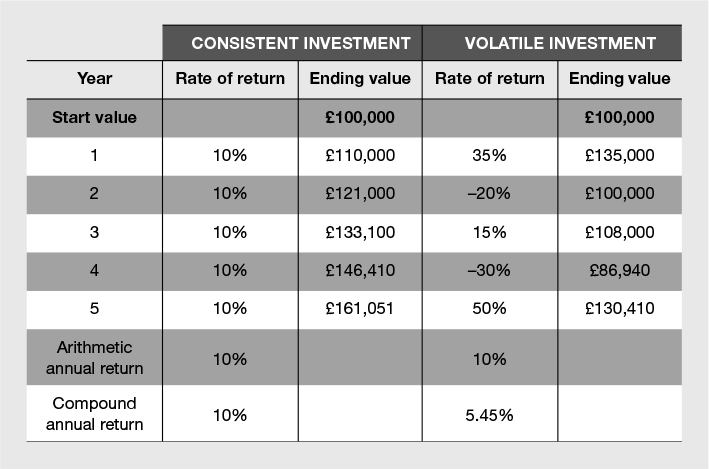
Figure 5.16 Impact of volatility on hypothetical £100,000 portfolio

We can calculate the probability of losing money from equity investment, in real terms (i.e. after inflation), in the future over different time periods by making an estimate of future expected investment returns and standard deviations. In Figure 5.17 you can see the results of a Monte Carlo simulation,¹⁶ which shows that, based on the data and assumptions used, the probability of losing money from equities over the long term is very low, but it’s likely that the investment experience to get there won’t be plain sailing. These risks need to be weighed up against the potential upside and the consequences of not receiving that upside had you never invested in equities in the first place.

Figure 5.17 Probability of losing money from equities

Source: Albion Strategic.

What’s right for me?

There is no ‘perfect’ portfolio and you need to take into account your life goals, income need, life expectancy and risk profile in helping to determine your asset allocation strategy. A prudent approach for most investors will be to diversify capital across the major asset classes. Figure 5.18 shows a range of possible portfolio allocations, along the risk–return spectrum, which might provide you with a reasonable starting place. If you are looking for your portfolio to provide a regular and rising income throughout your lifetime, your asset allocation decision will also need to take that into account.

Figure 5.18 Range of asset allocations

Table 5.3 shows historic risk–return simulations for a range of asset allocations, which allocate the equity across global markets for the period 1956–2013, to give you an idea of how they performed. However, do remember that the past is unlikely to be repeated and I suggest that in your plan assumptions you assume much lower investment returns (see Chapter 3 for my suggested investment assumptions).

Table 5.3 Historic risk-return simulations 1956–2013

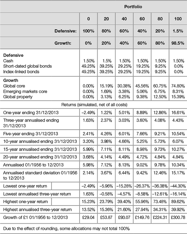
Source: Bloomsbury – calculated using Dimensional Returns 2.3. Asset class data have been used that represent close proxies for the asset classes included in the portfolio strategies. 1956 marks the starting point of this asset class data providing a reasonably informative proxy. As later asset class data become available, they are added into the calculation. Includes allowance for typical fund, custody and advice fees.