CHAPTER 12

OTHER INVESTMENT CONSIDERATIONS

Impact of dividends on overall investment returns

It is regularly stated that reinvested dividends make a big difference to overall equity investment returns over the medium to long term. This is well illustrated by Figure 12.1, which shows the FTSE All-Share Index with and without net dividends reinvested over the past 30 years.

I’ve heard some investment ‘experts’ suggest that high dividend-paying shares are better to own because they pay you for owning them and that in difficult investment conditions investors are somehow more likely to retain ownership of dividend-paying shares than those that pay no or a very low dividend. Research¹ suggests that high dividend-yielding stocks may be more risky and indeed the dividend may be high (when expressed as a percentage yield) because the price of the company has fallen. Dividends do not provide downside protection because current share prices reflect whether the earnings of a company have been paid out or retained. Dividends do not prevent encroaching on your capital because the distribution of dividends is reflected in companies’ share prices. The notion that owners of dividend-paying shares are somehow more committed shareholders may have some merit, but it is unlikely to be of any material consequence for most long-term investors.

Figure 12.1 Returns of the FTSE All-Share Index with and without dividends reinvested (returns for 30 years to 31 December 2013)

Source: Barclays Capital Equity Gilt Study 2014.

Another downside to focusing on companies that pay dividends, of whatever amount, is that you are highly likely to miss out on the significant investment returns arising from high-growth companies. Microsoft, Starbucks and Apple are just a few of the massive global companies that paid no dividends for many years. Highly profitable and fast-growing companies such as Amazon, eBay and Google still don’t. In both cases these companies’ share prices have grown much faster than those of many dividend-paying companies. The key point to appreciate is that whether companies pay dividends or not makes no difference to the total investment return, whereas the investment policy of the underlying investee companies will. Where dividends are paid, it makes sense to reinvest them to benefit from compounding, but specifically seeking out high-yielding shares is unlikely to give you the best investment outcome.

The impact of regular withdrawals from your portfolio

If you need your portfolio to fund your lifestyle over the long term, then you need to factor this into your investment strategy. The required amount of regular withdrawals, the portfolio’s time horizon (which may be your life expectancy), your risk profile and asset allocation are closely interrelated. If the amount regularly withdrawn from the portfolio is too high, you might run out of money before you die or not be able to leave a legacy. If the portfolio is too risky and suffers high volatility, the regular withdrawals may exacerbate the negative returns experienced during market downturns. Figure 12.2 illustrates this point well with the risky portfolio volatility being compounded by the regular withdrawals.

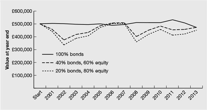
Figure 12.2 Effect of £15,000 p.a. withdrawals on portfolio value

There are a number of approaches that you could adopt when it comes to taking withdrawals from your investment portfolio and the right one will depend on your spending needs, investment strategy, risk profile and tax status.

• Natural yield. You take whatever interest or dividends are generated from the portfolio. Although the yield will vary from year to year, you could expect this to increase in real terms if you have made reasonable allocations to equities and property. Although initially this approach is likely to produce a relatively low level of income as a proportion of the portfolio, over the long term it should rise significantly.
• Fixed sum. You take a fixed monetary sum each year (e.g. £50,000) regardless of actual investment yield or overall returns. While this provides a constant level of ‘income’, it needs much closer monitoring, particularly if you have a reasonable allocation to risky assets and a high amount of withdrawal relative to the portfolio value. You may have to stop or reduce the amount withdrawn during market downturns.
• Percentage of portfolio. The withdrawal is expressed as a percentage of the portfolio, which may be higher or lower than the natural yield or overall return. The actual amount of withdrawals will vary up and down in line with fluctuations in the portfolio value, with higher allocations to risky assets leading to higher volatility in income withdrawals. However, the chances of running out of money with this approach are likely to be quite low, provided that the withdrawal percentage is not excessive.

If you need a stable level of cashflow from the portfolio, you could combine the fixed-amount and percentage-of-portfolio approaches. Such an approach could combine a fixed withdrawal based on a percentage average of, say, the past three years’ annual lifestyle expenditure with a percentage amount based on the portfolio value. You can weight these factors to favour your preference for either more stable cashflow or a greater chance of portfolio survival. This allows you to customise your withdrawals to smooth out consumption while responding to actual investment performance.

Example portfolios and withdrawal rates

A recent simplified analysis⁷ of the 4% rule, carried out for my firm, provides some useful insights into safe withdrawal rates. The analysis was based on a portfolio allocated 60% to equities and 40% to bonds, based on a range of 30-year historic performance outcomes as set out in Table 12.1. Note the wide range of 30-year returns and how they compare to the 113-year average.

Table 12.1 Balanced 60/40 portfolios: 30-year horizons (1900–2013) – annualised real returns

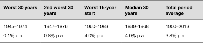
Data source: Barclays Equity Gilt Study 2014.

These return periods are plotted in Figure 12.3. The two worst time periods, perhaps not surprisingly, incorporate the worst one-year fall in 1974, effectively giving back much of the gain made up to that point. It is also worth noting that the purchasing power of gilts was substantially eroded by high inflation in the 1970s. This is a pretty extreme and tough test for the 4% rule.

These data were used to model a scenario of a 4% initial withdrawal rate on a £1 million portfolio. As the returns are in real terms, a constant £40,000 was withdrawn at the start of every year and the remaining portfolio value was indexed up by the real return that year. The purchasing power balances, over a 30-year period for the five different scenarios above, are plotted in Figure 12.4. The average return is equivalent to a straight-line approach to modelling future performance in a lifetime cashflow projection (see Chapter 3).

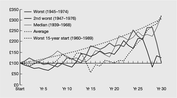
Figure 12.3 30-year return pathways in real terms

Source: Albion Strategic.

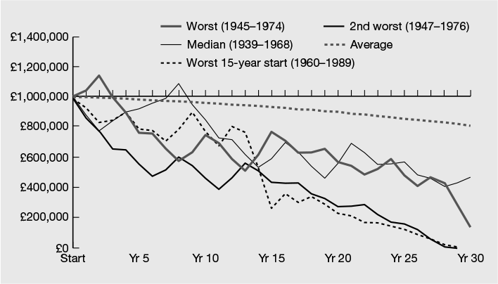
Figure 12.4 Impact on portfolio size withdrawing £40,000 p.a. (an initial 4% rate)

Source: Albion Strategic.

From this analysis we can make several observations:

• The two worst periods suffered badly, with the 2nd Worst scenario actually failing to survive through 30 years. The Worst portfolio did marginally better due to strong positive returns in the first two years of the sequence.
• The Median portfolio, despite delivering a comparable return of around 4% to the average return for the entire period of 3.8%, ended up with half the purchasing power it started with.
• The straight-line approach using the average return ended up with £800,000. The dangers surrounding a straight-line approach are evident.
• The Worst 15-year start scenario actually ran out of money despite returning more or less the same as the Median and the Average scenarios. This was because the portfolio had been eroded by withdrawals and poor market returns in the early years.

Fixed withdrawal strategy

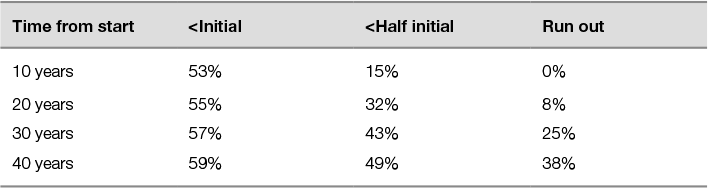
The analysis then modelled a 4% initial balance withdrawal strategy (i.e. £40,000 p.a.).⁸ A range of goals, and outcomes against these goals, is summarised in Table 12.2.

Table 12.2 Purchasing power outcomes of a 4% withdrawal strategy

Source: Albion Strategic.

It is evident that a 4% withdrawal rate is risky over a 30-year horizon, based on a portfolio with the parameters above, with a 25% chance of running out of money. The challenge is that for 75% of investors this strategy works. Simply reducing the withdrawal rate across the board to, say, 3% is a blunt tool as the majority of investors would be spending less than they need to. If the investor is working with a financial planning firm that reviews withdrawals at least annually, there is scope to adjust the withdrawal and plan, provided that the investor has the flexibility to do so. This illustrates the importance of having a range of annual lifestyle spending goals and an adequate cash reserve.

Dynamic withdrawal strategy

A similar analysis, but instead with a dynamic withdrawal rate (as per Tables 12.3 and 12.4), reduces the income withdrawal when the portfolio value falls below a certain target level.

Table 12.3 Dynamic withdrawal rate parameters

Rate of withdrawal	Upper limit	Lower level
4% of start value p.a.	No limit	80% of start value
3% of start value p.a.	<80%	>60%
2% of start value p.a.	<60%	No lower limit

Source: Analysis Albion Strategic.

Table 12.4 Purchasing power outcomes of a dynamic withdrawal strategy

Source: Analysis Albion Strategic.

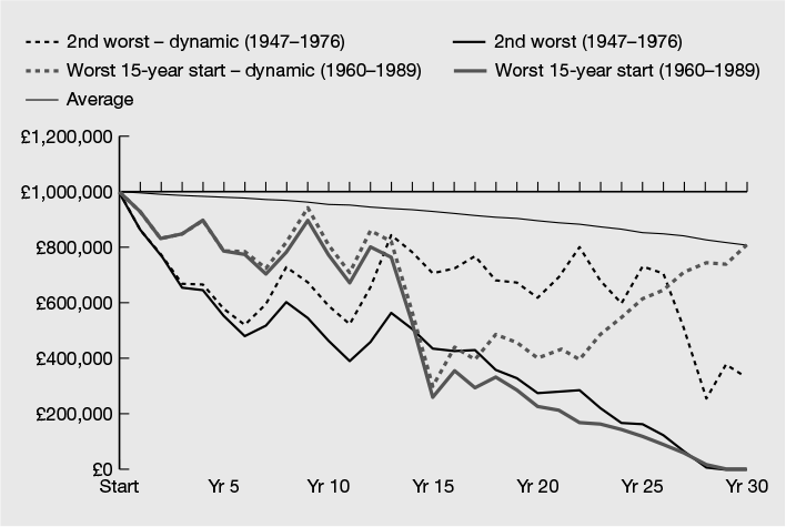
As can be seen from Figure 12.5, it is evident that the dynamic withdrawal strategy dramatically improves outcomes compared with a static withdrawal strategy, without penalising theoretical investment outcomes that are favourable.

Running a similar dynamic withdrawal analysis on the historical data scenarios of 2nd Worst and Worst 15-year start scenarios, which both failed at a static 4% withdrawal rate, we can see the positive impact it has on outcomes. Recent research by JP Morgan supports the adoption of a dynamic withdrawal strategy: ‘Based on this analysis, a dynamic withdrawal model may offer substantial advantages to help investors make the most of their assets throughout their retirement years.’⁹

Figure 12.5 Comparison of static vs. dynamic withdrawal rates

Source: Albion Strategic.

Interesting thoughts on asset allocation – the upward sloping equity glide path

A 2013 research paper¹⁰ suggests that investors should own the lowest allocation to equities at the time of retirement, as this is when they are most vulnerable to portfolio losses. Beyond that point, the allocation should rise to help to increase the chances of the pot surviving the investor. If equity markets do badly in the early years, the investor will not have suffered the full brunt of any fall and will, by averaging their way into the equity market over time, benefit from any market recovery. If equity markets have done well in the early years, there will be little concern. This strategy has been dubbed a ‘rising equity glide path’ by the authors and is counter to the perceived wisdom that the older one gets, the lower the allocation to equities should be.

Determining the right portfolio withdrawal strategy

While there is no single answer, there are some principles that you can use to help you determine and manage the right portfolio withdrawal strategy.

• Historic average investment returns disguise the fact that such returns are not delivered in a consistent manner and, depending on the investment strategy adopted, will vary from year to year. This means that any financial modelling done to determine a sustainable regular withdrawal strategy, on the basis of average annual investment return assumptions, may overstate the viability.
• Plan viability is greatly affected if regular withdrawals are high in the first five years or so and the portfolio suffers significant volatility and/or a fall in value.
• Risk analysis systems such as Monte Carlo modelling can provide useful insights into the probability of portfolio sustainability, but oversimplify the outcome as either success or failure. In reality, all of the assumptions together will almost certainly prove to be wrong, and the plan (such as annual withdrawals) can be modified well before the plan gets into danger territory.
• It is likely to be helpful to model lower rates of return and/or lower levels of annual withdrawals, to gain a better insight into plan viability.
• Some of the more sophisticated planning tools allow the portfolio withdrawals to be stress tested in the event of a major stock market crash at different stages of the plan.
• A dynamic portfolio withdrawal strategy, based on rules along the lines of those set out in this chapter, is likely to improve the probability of the portfolio surviving across a range of investment return outcomes.
• The highest chance of success and most efficient use of capital is likely to arise if regular withdrawals are and remain low (<2.5% p.a.) in proportion to the portfolio value and the investment strategy has a low-risk profile (i.e. with low volatility).
• Assuming that the portfolio will be investing entirely in index-linked gilts and a low withdrawal rate will be taken (broadly equivalent to the natural yield) seems to be a sensible base scenario to compare with other withdrawal strategies, as this represents a low-risk option for an investor whose liabilities (i.e. future expenditure) are expected to increase with inflation.
• If you have a long time horizon and expenditure that rises much faster than official inflation, coupled with a low equity allocation, this will translate into a high probability of declining consumption in the long term (i.e. withdrawals will have to be reduced at some stage) to avoid the portfolio being exhausted.
• Expected final values are higher for portfolios with high equity allocations, but so is the likelihood of leaving a small legacy. This is a classic risk–return trade-off.
• Whether you adopt a static or dynamic withdrawal strategy, it is essential to review the withdrawal level periodically (no less than tri-annually) in the light of actual investment returns achieved and make adjustments as necessary. This is particularly important for portfolios with higher levels of withdrawals, regardless of their exposure to risky assets and to portfolios with high allocations to equities with moderate to high levels of withdrawals.

Adding risky assets to a portfolio is done in the expectation, but not the certainty, that it will generate real returns in excess of those available from cash and index-linked gilts. As an investor you need to weigh up the probability of running out of money in your lifetime against the alternative of a less expensive lifestyle.

The importance of rebalancing your portfolio

As we’ve already discussed, your portfolio’s asset allocation is one of the most important decisions in the portfolio-construction process and is the major determinant of its risk–return characteristics. How the portfolio is taxed can also have a big impact on how much of those returns you keep. With a multi-asset class portfolio that uses collective funds, over time, each asset class will generate different returns, which will cause your portfolio’s asset allocation and consequently its risk profile to change. This is known as portfolio drift and is unlikely to be consistent with your goals, preferences and tax position. The portfolio will, therefore, require some ongoing management and review to manage both risks and taxes.

Sometimes an asset class can experience significant volatility over a time period but end it at the same value as that at which it started. Take, for example, the Japanese stock market as represented by the Nikkei 225 Index for the 29 years ending 2013. As you can see from Figure 12.6, the index experienced many large rises and falls, some of which were more than 100%.

A disciplined rebalancing policy forces you to sell high and buy low. This doesn’t remove risk but maintains the risk exposure (which is after all the source of additional returns) that you set at the outset. In order to re-establish the portfolio’s original risk and return characteristics, it needs to be rebalanced so that each holding reflects the original asset allocation. All other things being equal, a regularly rebalanced portfolio will maintain the risk–reward characteristics of the target asset allocation compared with a portfolio that is never rebalanced. An optimally rebalanced portfolio is likely to produce a similar return to that of a non-rebalanced portfolio but at a lower level of risk. See Figure 12.7.

Figure 12.6 Performance of the Nikkei 225 Index (29 years ending 2013)

Figure 12.7 Comparison of rebalanced and non-rebalanced portfolios

An additional benefit of rebalancing a taxable portfolio is that it enables gains and losses to be crystallised, which can help with minimising tax. In practice, a sensible rebalancing strategy forces you to reduce exposure to those asset classes that have performed relatively well compared with the others you hold, in favour of asset classes that have performed relatively poorly and/or fallen in value. This ‘sell high and buy low’ discipline is the opposite of what most retail (and many institutional) investors do, because taking profits and buying more of an asset class that has fallen in value is difficult for most people to do, due to their emotional response to losses and gains. However, logically, if an asset has fallen in value, then its expected return increases, and if it has risen in value, its expected return falls.

In the same way that there is no ‘perfect’ asset allocation, there is no ‘perfect’ rebalancing approach. In developing your rebalancing strategy you need to consider three key questions.

The mechanics of rebalancing

The simplest way of rebalancing your portfolio is to use new cash to invest in those assets that are underweight. This cash might come from additional capital being added to the portfolio or, more likely, from accumulated interest and dividends arising from the portfolio holdings. For this reason it is important to avoid investing in any funds that automatically reinvest interest and dividends. By using cash to rebalance you will reduce the number of transactions that you or your adviser will need to carry out and, in the case of portfolios that are taxable, you’ll avoid unnecessary crystallisation of taxable capital gains.

The other method of rebalancing is to realise cash from the overweight portfolio holdings to reinvest in the underweight holdings. In the case of taxable portfolios, this might be more attractive than using new cash if you need to crystallise gains to utilise your annual capital gains tax exemption or crystallise losses to offset against current year gains or to be carried forward for use in future tax years.

If a large, taxable capital gain would arise as a result of rebalancing back to the exact allocation, you might wish to rebalance to as near to the model as you can without crystallising the extra tax. Alternatively, you might wish to delay the rebalancing if you anticipate being able to add more capital to the portfolio in the near term or expect to be a basic-rate taxpayer in the next tax year, but don’t fall into the trap of letting tax overly influence the need to rebalance. The most tax-efficient portfolio is one that makes only losses and if you don’t rebalance, particularly when markets have risen sharply, you might see those gains evaporate, as we saw earlier with the Japanese stock market. I remember as far back as the late 1990s when many investors were unwilling to sell out of their technology stocks because of the tax they would have paid. Although continuing to hold them through 2001 certainly avoided the tax problem, the collateral damage to their portfolios when the sector corrected spectacularly may have given rise to a few regrets.

Most people with reasonable-sized portfolios are likely to have taxed and non-taxed elements. It is likely, therefore, that a combination of using cash (whether from interest/dividends or additional investment capital) and releasing cash from other holdings will be necessary to carry out rebalancing.

The use of debt with investing

Depending on your point of view, debt is either something to be avoided at all costs or a useful way of multiplying wealth and opportunity. The two most common questions about debt are:

1. Should I use capital/income to pay down debt or should I invest?
2. Should I use debt to augment my investment capital to leverage higher investment returns?

Debt is a negative bond (fixed-income) exposure, although the interest costs will invariably be higher than the interest rate earned on bonds. So if you have a £200,000 bond and £200,000 equity exposure in your investment portfolio, e.g. 50% to each asset class and a £50,000 mortgage, your actual bond exposure is £150,000 (the bond of £200,000 less the £50,000 mortgage). The result is that instead of having 50% of your portfolio allocated to risky equities you actually have 57%. This higher risk might be acceptable if you have a need and tolerance for a higher allocation to risky assets.

Figure 12.8 Portfolio rebalancing decision-making framework

It is unlikely that you will be able to earn a higher rate of interest from cash or bonds in taxable accounts, particularly for higher- and additional-rate taxpayers, than the cost of interest on a mortgage. Repaying debt is a risk-free return whereas a taxable investment would need to deliver a higher return than the risk-free rate and, as such, would be risky. In Table 12.5 you can see a range of mortgage rates and the taxable rate of return that you would need to obtain at different tax rates just to break even.

Table 12.5 Gross investment returns required to equal mortgage interest costs

In tax-free and tax-deferred accounts such as ISAs and offshore investment bonds, the position is more finely balanced. However, on tax-favoured accounts such as pensions, particularly where initial tax relief is obtained at a higher rate on the contribution than is payable on benefits and tax-efficient growth is achieved in the intervening period, it can be highly attractive not to repay debt and instead make pension contributions (see Chapter 17 on pensions).

Inflation and deflation

A variable-rate loan is fully exposed to inflationary pressures and one would expect rates to rise or remain high in an environment of rising or strong inflation. If you think that deflation is more likely, then a variable-rate loan makes more sense as the cost of borrowing is likely to fall to nil. However, in that situation, any real assets, such as property or equities, that the loan may have been used to purchase are also likely to experience a fall in value. A fixed-rate loan, meanwhile, is protected against rising inflation but will be exposed to deflation unless the loan includes the option to repay some of it or the entire amount early without penalty.

Leverage amplifies gains and losses

Borrowing allows you to leverage returns on investment capital. This is great when the asset or business is going up in value, because the return over the cost of the debt is added to the investor’s capital as ‘free’ excess return. However, debt can also amplify losses, as many people and companies have found out since the financial crisis of 2007–2009 began to unwind.

For those with significant wealth, the most common use of debt is as investment in property, because fractional ownership of physical property is not feasible in most cases in the same way as it is with equities and bonds. In addition, debt can be introduced to a property portfolio, for example, to allow capital to be extracted tax-efficiently, with the rental income servicing the interest. If you want to retain the property as an investment but have a better use for some of the equity, this could be a good idea.

There is a multitude of packaged investments that come with inbuilt leverage, which serves to increase the relative risks compared with unleveraged investment in, say, an equity index fund. Examples of such investments are as follows:

• investment trusts (see Chapter 11)
• property funds
• property partnerships and syndicates
• enterprise zone property syndicates (no new schemes are available)
• business premises renovation allowance syndicates
• affordable housing partnerships
• film partnerships
• carbon/clean energy funds
• long/short 130 equity funds.

In some cases, the debt is required to obtain a tax effect, such as with business premises renovation allowance syndicates, whereas with others, such as the long/short 130 equity fund,¹² it is required to generate the expected return. The key point to remember is that once you adjust the expected return for the additional risk of debt, you are likely to end up with a return similar, or in some cases lower, than that from an unleveraged investment portfolio.

Later life needs

Debt can also be used as part of later life planning. Those who need to fund lifestyle expenditure and/or care fees funding, but who have insufficient liquid assets and/or income, could use what is known as a lifetime mortgage secured against their property. In most cases the interest is rolled up and added to the loan until the borrower’s death, when the loan is repaid from the proceeds arising from selling the property. Most lenders active in this market give a guarantee that the loan and rolled-up interest will never be more than the value of the property, known as a ‘no negative equity guarantee’. For this reason the maximum loan is usually less than 50% of the property value, but the actual amount depends on the borrower’s age and the lender’s interest rate.

Lifetime mortgages are a relatively expensive way of funding later life needs but can be a viable option for individuals who wish to remain in their own home, have no other assets on which to call and don’t wish (or are unable) to borrow funds on similar terms from other family members. In addition to your willingness and need to take risks, using debt in your wealth plan boils down to your need to ‘sleep well’. Those at the beginning of their earning capacity and those nearing the end of their life can usually cope with debt more than those with other age and wealth profiles. However, if you are looking to preserve what you have in real terms and want as few moving parts as possible in your investment approach, avoid debt as far as possible.