
Chapter 10
Going Beyond Select Queries
IN THIS CHAPTER
- Working with aggregate queries
- Using action queries
- Creating crosstab queries
- Optimizing query performance
- Retrieving and displaying specific records with a select query is indeed a fundamental task when analyzing data in Access. However, it's just a small portion of what makes up data analysis. The scope of data analysis is broad and includes grouping and comparing data, updating and deleting data, performing calculations on data, and shaping and reporting data. Access has built-in tools and functionalities designed specifically to handle each of these tasks.
In this chapter, we give you an in-depth look at the various tools available to you in Access and how they can help you go beyond select queries.
Aggregate Queries
An aggregate query, sometimes referred to as a group-by query, is a type of query you can build to help you quickly group and summarize your data. With a select query, you can retrieve records only as they appear in your data source. But with an aggregate query, you can retrieve a summary snapshot of your data that shows you totals, averages, counts, and more.
Creating an aggregate query
To get a firm understanding of what an aggregate query does, consider the following scenario: You've just been asked to provide the sum of total revenue by period. In response to this request, start a query in Design view and bring in the Dim_Dates.Period and Dim_Transactions.LineTotal fields, as shown in Figure 10.1. If you run this query as is, you'll get every record in your dataset instead of the summary you need.

Figure 10.1 Running this query will return all the records in your dataset, not the summary you need.
In order to get a summary of revenue by period, you'll need to activate Totals in your design grid. To do this, go to the Ribbon and select the Design tab, and then click the Totals button. As you can see in Figure 10.2, after you've activated Totals in your design grid, you'll see a new row in your grid called Total. The Total row tells Access which aggregate function to use when performing aggregation on the specified fields.

Figure 10.2 Activating Totals in your design grid adds a Total row to your query grid that defaults to Group By.
Notice that the Total row contains the words Group By under each field in your grid. This means that all similar records in a field will be grouped to provide you with a unique data item. We'll cover the different aggregate functions in depth later in this chapter.
The idea here is to adjust the aggregate functions in the Total row to correspond with the analysis you're trying perform. In this scenario, you need to group all the periods in your dataset, and then sum the revenue in each period. Therefore, you'll need to use the Group By aggregate function for the Period field, and the Sum aggregate function for the LineTotal field.
Since the default selection for Totals is the Group By function, no change is needed for the Period field. However, you'll need to change the aggregate function for the LineTotal field from Group By to Sum. This tells Access that you want to sum the revenue figures in the LineTotal field, not group them. To change the aggregate function, simply click the Totals drop-down list under the LineTotal field, shown in Figure 10.3, and select Sum. At this point, you can run your query.

Figure 10.3 Change the aggregate function under the LineTotal field to Sum.
As you can see in Figure 10.4, the resulting table gives a summary of your dataset, showing total revenue by period.
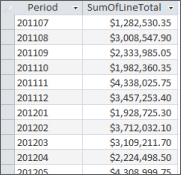
Figure 10.4 After running your query, you have a summary showing your total revenue by period.
About aggregate functions
In the example shown in Figure 10.3, you selected the Sum aggregate function from the Totals drop-down list. Obviously, you could've selected any one of the 12 functions available. Indeed, you'll undoubtedly come across analyses where you'll have to use a few of the other functions available to you. So, it's important to know what each one of these aggregate functions means for your data analysis.
Group By
The Group By aggregate function aggregates all the records in the specified field into unique groups. Here are a few things to keep in mind when using the Group By aggregate function:
- Access performs the
Group Byfunction in your aggregate query before any other aggregation. If you're performing aGroup Byalong with another aggregate function, theGroup Byfunction will be performed first. The example shown in Figure 10.4 illustrates this concept. Access groups the Period field before summing the LineTotal field. - Access sorts each group-by field in ascending order. Unless otherwise specified, any field tagged as a group-by field will be sorted in ascending order. If your query has multiple group-by fields, each field will be sorted in ascending order starting with the leftmost field.
- Access treats multiple group-by fields as one unique item. To illustrate this point, create a query that looks similar to the one shown in Figure 10.5. This query counts all the transactions that were logged in the 201201 period.

Figure 10.5 This query returns only one line showing total records for the 201201 period.
Now return to the Query Design view and add ProductID, as shown here in Figure 10.6. This time, Access treats each combination of Period and Product Number as a unique item. Each combination is grouped before the records in each group are counted. The benefit here is that you've added a dimension to your analysis. Not only do you know how many transactions per ProductID were logged in 201201, but if you add up all the transactions, you'll get an accurate count of the total number of transactions logged in 201201.

Figure 10.6 This query results in a few more records, but if you add up the counts in each group, they'll total 503.
Sum, Avg, Count, StDev, Var
These aggregate functions all perform mathematical calculations against the records in your selected field. It's important to note that these functions exclude any records that are set to null. In other words, these aggregate functions ignore any empty cells.
Sum:Calculates the total value of all the records in the designated field or grouping. This function will work only with the following data types: AutoNumber, Currency, Date/Time, and Number.Avg: Calculates the average of all the records in the designated field or grouping. This function will work only with the following data types: AutoNumber, Currency, Date/Time, and Number.Count: Counts the number of entries within the designated field or grouping. This function works with all data types.StDev: Calculates the standard deviation across all records within the designated field or grouping. This function will work only with the following data types: AutoNumber, Currency, Date/Time, and Number.Var: Calculates the amount by which all the values within the designated field or grouping vary from the average value of the group. This function will work only with the following data types: AutoNumber, Currency, Date/Time, and Number.
Min, Max, First, Last
Unlike other aggregate functions, these functions evaluate all the records in the designated field or grouping and return a single value from the group.
Min: Returns the value of the record with the lowest value in the designated field or grouping. This function will work only with the following data types: AutoNumber, Currency, Date/Time, Number, and Text.Max: Returns the value of the record with the highest value in the designated field or grouping. This function will work only with the following data types: AutoNumber, Currency, Date/Time, Number, and Text.First: Returns the value of the first record in the designated field or grouping. This function works with all data types.Last: Returns the value of the last record in the designated field or grouping. This function works with all data types.
Expression, Where
One of the steadfast rules of aggregate queries is that every field must have an aggregation performed against it. However, in some situations you'll have to use a field as a utility—that is, use a field to simply perform a calculation or apply a filter. These fields are a means to get to the final analysis you're looking for, rather than part of the final analysis. In these situations, you'll use the Expression function or the Where clause. The Expression function and the Where clause are unique in that they don't perform any grouping action per se.
Expression: TheExpressionaggregate function is generally applied when you're utilizing custom calculations or other functions in an aggregate query.Expressiontells Access to perform the designated custom calculation on each individual record or group separately.Where: TheWhereclause allows you to apply a criterion to a field that is not included in your aggregate query, effectively applying a filter to your analysis.
To see the Expression aggregate function in action, create a query in Design view that looks like the one shown in Figure 10.7. Note that you're using two aliases in this query: “Revenue” for the LineTotal field and “Cost” for the custom calculation defined here. Using an alias of “Revenue” gives the sum of LineTotal a user-friendly name.

Figure 10.7 The Expression aggregate function allows you to perform the designated custom calculation on each Period group separately.
Now you can use [Revenue] to represent the sum of LineTotal in your custom calculation. The Expression aggregate function ties it all together by telling Access that [Revenue]*.33 will be performed against the resulting sum of LineTotal for each individual Period group. Running this query will return the total Revenue and Cost for each Period group.
To see the Where clause in action, create a query in Design view that looks like the one shown in Figure 10.8. As you can see in the Total row, you're grouping ProductID and summing LineTotal. However, Period has no aggregation selected because you only want to use it to filter out one specific period. You've entered 201201 in the criteria for Period. If you run this query as is, you'll get the following error message: You tried to execute a query that does not include the specified expression 'Period' as part of an aggregate function.

Figure 10.8 Running this query will cause an error message because you have no aggregation defined for Period.
To run this query successfully, click the Totals drop-down list for the Period field and select Where. At this point, your query should look similar to the one shown here in Figure 10.9. With the Where clause specified, you can successfully run this query.
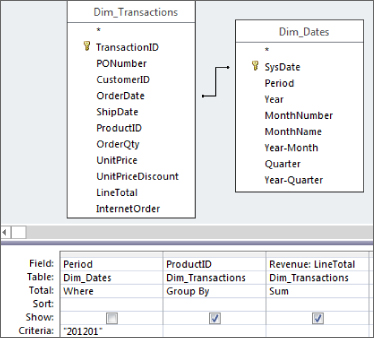
Figure 10.9 Adding a Where clause remedies the error and allows you to run the query.
Action Queries
As we mentioned earlier, in addition to querying data, the scope of data analysis includes shaping data, changing data, deleting data, and updating data. Access provides action queries as data analysis tools to help you with these tasks. Unfortunately, many people don't use these tools; instead, they export small chunks of data to Excel to perform these tasks. That may be fine if you're performing these tasks as a one-time analysis with a small dataset. But what do you do when you have to carry out the same analysis on a weekly basis, or if the dataset you need to manipulate exceeds Excel's limits? In these situations, it would be impractical to routinely export data into Excel, manipulate the data, and then re-import the data back into Access. Using action queries, you can increase your productivity and reduce the chance of errors by carrying out all your analytical processes within Access.
You can think of an action query the same way you think of a select query. Like a select query, an action query extracts a dataset from a data source based on the definitions and criteria you pass to the query. The difference is that when an action query returns results it doesn't display a dataset; instead, it performs some action on those results. The action it performs depends on its type.
There are four types of action queries: make-table queries, delete queries, append queries, and update queries. Each query type performs a unique action.
Make-table queries
A make-table query creates a new table consisting of data from an existing table. The table that is created consists of records that have met the definitions and criteria of the make-table query.
In simple terms, if you create a query, and you want to capture the results of your query in its own table, you can use a make-table query to create a hard table with your query results. Then you can use your new table in some other analytical process.
Let's say you've been asked to provide the marketing department with a list of customers, along with information on each customer's sales history. A make-table query will get you the data you need. To create a make-table query, follow these steps:
- Create a query in the Query Design view that looks similar to the one shown in Figure 10.10.

Figure 10.10 Create this query in Design view.
- Select the Design tab of the Ribbon, and then click the Make Table button. The Make Table dialog box (shown in Figure 10.11) appears.

Figure 10.11 Enter the name of your new table.
- In the Table Name field, enter the name you want to give to your new table. For this example, type SalesHistory. Be sure not to enter the name of a table that already exists in your database, because it'll be overwritten.
- Click OK to close the dialog box, and then click the Run command to run your query. Access throws up the warning message shown in Figure 10.12, letting you know that you won't be able to undo this action.
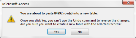
Figure 10.12 Click Yes to run your query.
- Click Yes to confirm and create your new table.
When your query has finished running, you'll find a new table called SalesHistory in your Table objects.
Delete queries
A delete query deletes records from a table based on the definitions and criteria you specify. That is, a delete query affects a group of records that meet a specified criterion that you apply.
Although you can delete records by hand, in some situations using a delete query is more efficient. For example, if you have a very large dataset, a delete query deletes your records faster than a manual delete can. In addition, if you want to delete certain records based on several complex criteria, you'll want to use a delete query. Finally, if you need to delete records from one table based on a comparison to another table, a delete query is the way to go.
Given the fact that deleted data can't be recovered, get in the habit of taking one of the following actions in order to avoid a fatal error:
- Run a select query to display the records you're about to delete. Then review the records to confirm that these records are indeed the ones you want to delete, and then run the query as a delete query.
- Run a select query to display the records you're about to delete. Then change the query into a make-table query. Run the make-table query to make a backup of the data you're about to delete. Finally, run the query again as a delete query to delete the records.
- Make a backup of your database before running your delete query.
Now let's say the marketing department has informed you that the SalesHistory table you gave them includes records that they don't need. They want you to delete all history before the 201206 Period. A delete query based on the SalesHistory table you created a moment ago will accomplish this task. To create a delete query, follow these steps:
- Bring in the Period field and enter <PD201206 in the Criteria row. Access will automatically add quotations around your criteria. Your design grid should look like the one shown in Figure 10.13.

Figure 10.13 This query will select all records with a Period earlier than 201206.
- Perform a test by running the query.
- Review the records that are returned, and take note that 2,781 records meet your criteria. You now know that 2,781 records will be deleted if you run a delete query based on these query definitions.
- Return to Design view.
- Select the Design tab of the Ribbon, and then click the Delete button.
- Run your query again. Access throws up the message shown in Figure 10.14, telling you that you're about to delete 2,781 rows of data and warning you that you won't be able to undo this action. This is the number you were expecting to see, because the test you ran earlier returned 2,781 records.

Figure 10.14 Click Yes to continue with your delete action.
- Because everything checks out, click Yes to confirm and delete the records.
Append queries
An append query appends records to a table based on the definitions and criteria you specify in your query. In other words, with an append query, you can add the results of your query to the end of a table, effectively adding rows to the table.
With an append query, you're essentially copying records from one table or query and adding them to the end of another table. Append queries come in handy when you need to transfer large datasets from one existing table to another. For example, if you have a table called Old Transactions in which you archive your transaction records, you can add the latest batch of transactions from the New Transactions table simply by using an append query.
There are generally two reasons why records can get lost during an append process:
- Type conversion failure: This failure occurs when the character type of the source data doesn't match that of the destination table column. For example, imagine that you have a table with a field called Cost. Your Cost field is set as a Text character type because you have some entries that are tagged as TBD (to be determined), because you don't know the cost yet. If you try to append that field to another table whose Cost field is set as a Number character type, all the entries that have TBD will be changed to null, effectively deleting your TBD tag.
- Key violation: This violation occurs when you're trying to append duplicate records to a field in the destination table that is set as a primary key or is indexed as No Duplicates. In other words, when you have a field that prohibits duplicates, Access won't let you append any record that is a duplicate of an existing record in that field.
Another hazard of an append query is that the query will simply fail to run. There are two reasons why an append query will fail:
- Lock violation: This violation occurs when the destination table is open in Design view or is opened by another user on the network.
- Validation rule violation: This violation occurs when a field in the destination table has one of the following property settings:
- Required field is set to Yes: If a field in the destination table has been set to Required Yes and you don't append data to this field, your append query will fail.
- Allow Zero Length is set to No: If a field in the destination table has been set to Zero Length No and you don't append data to this field, your append query will fail.
- Validation rule set to anything: If a field in the destination table has a validation rule and you break the rule with your append query, your append query will fail. For example, if you have a validation rule for the Cost field in your destination table set to >0, you can't append records with a quantity less than or equal to zero.
Luckily, Access will clearly warn you if you're about to cause any of these errors. Figure 10.15 demonstrates this warning message, which tells you that you can't append all the records due to errors. It also tells you exactly how many records won't be appended because of each error. In this case, 5,979 records won't be appended because of key violations. You have the option of clicking Yes or No. If you click Yes, the warning is ignored and all records are appended, minus the records with the errors. If you click No, the query will be canceled, which means that no records will be appended.

Figure 10.15 The warning message tells you that you'll lose records during the append process.
Let's say the marketing department tells you that they made a mistake—they actually need all the sales history for the 2012 fiscal year. So, they need periods 201201 thru 201205 added back to the SalesHistory report. An append query is in order.
In order to get them what they need, follow these steps:
- Create a query in the Query Design view that looks similar to the one shown in Figure 10.16.
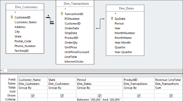
Figure 10.16 This query selects all records contained in Periods 201201 thru 201205.
- Select the Design tab of the Ribbon, and then click the Append button. The Append dialog box (shown in Figure 10.17) appears.

Figure 10.17 Enter the name of the table to which you want to append your query results.
- In the Table Name field, enter the name of the table to which you would like to append your query results. In this example, enter SalesHistory.
- Once you've entered your destination table's name, click OK. Your query grid has a new row called Append To under the Sort row (see Figure 10.18). The idea is to select the name of the field in your destination table where you want to append the information resulting from your query. For example, the Append To row under the Period field shows the word Period. This means that the data in the Period field of this query will be appended to the Period field in the SalesHistory table.

Figure 10.18 In the Append To row, select the name of the field in your destination table where you want to append the information resulting from your query.
- Run your query. Access throws up a message, as shown in Figure 10.19, telling you that you're about to append 2,781 rows of data and warning you that you won't be able to undo this action.

Figure 10.19 Click Yes to continue with your append action.
- Click Yes to confirm and append the records.
Update queries
The primary reason to use update queries is to save time. There is no easier way to edit large amounts of data at one time than with an update query. For example, imagine you have a Customers table that includes customers' zip codes. If the zip code 32750 has been changed to 32751, you can easily update your Customers table to replace 32750 with 32751.
Let's say you've just received word that the zip code for all customers in the 33605 zip code has been changed to 33606. In order to keep your database accurate, you'll have to update all the 33605 zip codes in your Dim_Customers table to 33606. Here's how:
- Create a query in the Query Design view that looks similar to the one shown in Figure 10.20.
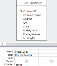
Figure 10.20 This query will select all customers that are in the 33605 zip code.
- Perform a test by running the query.
- Review the records that are returned, and take note that six records meet your criteria. You now know that six records will be updated if you run an update query based on these query definitions.
- Return to the Design view.
- Select the Design tab of the Ribbon, and click the Update button. Your query grid now has a new row called Update To. The idea is to enter the value to which you would like to update the current data. In this scenario, shown in Figure 10.21, you want to update the zip code for the records you're selecting to 33606.

Figure 10.21 In this query, you are updating the zip code for all customers that have a code of 33605 to 33606.
- Run the query. Access throws up the message shown in Figure 10.22, telling you that you're about to update six rows of data and warning you that you won't be able to undo this action. This is the number you were expecting to see, because the test you ran earlier returned six records.

Figure 10.22 Click Yes to continue with your update action.
- Since everything checks out, click Yes to confirm and update the records.
Crosstab Queries
A crosstab query is a special kind of aggregate query that summarizes values from a specified field and groups them in a matrix layout by two sets of dimensions, one set down the left side of the matrix and the other set listed across the top of the matrix. Crosstab queries are perfect for analyzing trends over time or providing a method for quickly identifying anomalies in your dataset.
The anatomy of a crosstab query is simple. You need a minimum of three fields in order to create the matrix structure that will become your crosstab. The first field makes up the row headings; the second field makes up the column headings; and the third field makes up the aggregated data in the center of the matrix. The data in the center can represent a Sum, Count, Average, or any other aggregate function. Figure 10.23 demonstrates the basic structure of a crosstab query.
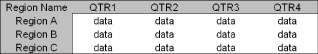
Figure 10.23 The basic structure of a crosstab query.
There are two methods to create a crosstab query. You can use the Crosstab Query Wizard or create a crosstab query manually using the query design grid.
Creating a crosstab query using the Crosstab Query Wizard
To use the Crosstab Query Wizard to create a crosstab query, follow these steps:
- Select the Create tab of the Ribbon and then click the Query Wizard button. The New Query dialog box, shown in Figure 10.24, appears.
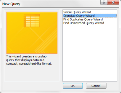
Figure 10.24 Select Crosstab Query Wizard from the New Query dialog box.
- Select Crosstab Query Wizard from the selection list, and then click OK.
The first step in the Crosstab Query Wizard is to identify the data source you'll be using. As you can see in Figure 10.25, you can choose either a query or a table as your data source. In this example, you'll be using the Dim_Transactions table as your data source.

Figure 10.25 Select the data source for your crosstab query.
- Select Dim_Transactions and then click the Next button.
The next step is to identify the fields you want to use as the row headings.
- Select the ProductID field and click the button with the > symbol on it to move it to the Selected Items list. The dialog box should look like Figure 10.26. Notice that the ProductID field is shown in the sample diagram at the bottom of the dialog box.
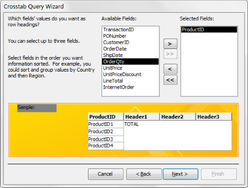
Figure 10.26 Select the ProductID field and then click the Next button.
You can select up to three fields to include in your crosstab query as row headings. Remember that Access treats each combination of headings as a unique item. That is, each combination is grouped before the records in each group are aggregated.
The next step is to identify the field you want to use as the column heading for your crosstab query. Keep in mind that there can be only one column heading in your crosstab.
- Select the OrderDate field from the field list. Notice in Figure 10.27 that the sample diagram at the bottom of the dialog box updates to show the OrderDate.

Figure 10.27 Select the OrderDate field then click the Next button.
If your Column Heading is a date field, as the OrderDate is in this example, you'll see the step shown in Figure 10.28. In this step, you'll have the option of specifying an interval to group your dates by.

Figure 10.28 Select Quarter and then click Next.
- Select Quarter and notice that the sample diagram at the bottom of the dialog box updates accordingly.
You're almost done. In the second-to-last step, shown in Figure 10.29, you'll identify the field you want to aggregate and the function you want to use.
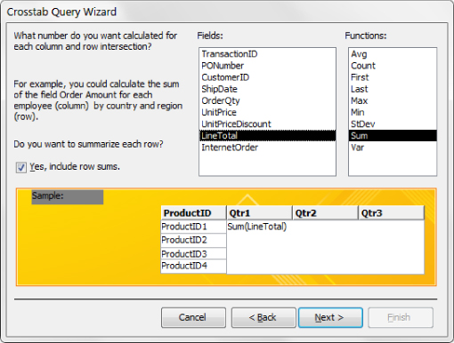
Figure 10.29 Select the LineTotal and Sum, and then click the Next button.
- Select the LineTotal field from the Fields list, and then select Sum from the Functions list. Notice the Yes, Include Row Sums check box. This box is checked by default to ensure that your crosstab query includes a Total column that contains the sum total for each row. If you don't want this column, simply remove the check from the check box.
If you look at the sample diagram at the bottom of the dialog box, you will get a good sense of what your final crosstab query will do. In this example, your crosstab will calculate the sum of the LineTotal field for each ProductID by Quarter.
The final step, shown in Figure 10.30, is to name your crosstab query.

Figure 10.30 Click Finish to see your query results.
- In this example, name your crosstab Product Summary by Quarter. After you name your query, you have the option of viewing your query or modifying the design.
- In this case, you want to view your query results so simply click the Finish button.
In just a few clicks, you've created a powerful look at the revenue performance of each product by quarter (see Figure 10.31).

Figure 10.31 A powerful analysis in just a few clicks.
Creating a crosstab query manually
Although the Crosstab Query Wizard makes it easy to create a crosstab in just a few clicks, it does have limitations that may inhibit your data analysis efforts:
- You can select only one data source on which to base your crosstab. This means that if you need to crosstab data residing across multiple tables, you'll need to take extra steps to create a temporary query to use as your data source.
- There is no way to filter or limit your crosstab query with criteria from the Crosstab Query Wizard.
- You're limited to only three row headings.
- You can't explicitly define the order of your column headings from the Crosstab Query Wizard.
The good news is that you can create a crosstab query manually through the query design grid. Manually creating your crosstab query allows you greater flexibility in your analysis.
Using the query design grid to create your crosstab query
Here's how to create a crosstab query using the query design grid:
- Create the aggregate query shown in Figure 10.32. Notice that you're using multiple tables to get the fields you need. One of the benefits of creating a crosstab query manually is that you don't have to use just one data source—you can use as many sources as you need in order to define the fields in your query.

Figure 10.32 Create an aggregate query as shown here.
- Select the Design tab of the Ribbon and click the Crosstab button. A row called Crosstab has been added to your query grid (see Figure 10.33). The idea is to define what role each field will play in your crosstab query.
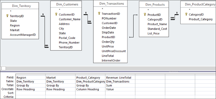
Figure 10.33 Set each field's role in the Crosstab row.
- Under each field in the Crosstab row, select whether the field will be a row heading, a column heading, or a value.
- Run the query to see your crosstab in action.
When building your crosstab in the query grid, keep the following in mind:
- You must have a minimum of one row heading, one column heading, and one value field.
- You can't define more than one column heading.
- You can't define more than one value heading.
- You are not limited to only three row headings.
Customizing your crosstab queries
As useful as crosstab queries can be, you may find that you need to apply some of your own customizations in order to get the results you need. In this section, we explain a few of the ways you can customize your crosstab queries to meet your needs.
Defining criteria in a crosstab query
The ability to filter or limit your crosstab query is another benefit of creating crosstab queries manually. To define a filter for your crosstab query, simply enter the criteria as you normally would for any other aggregate query. Figure 10.34 demonstrates this concept.

Figure 10.34 You can define a criterion to filter your crosstab queries.
Changing the sort order of your crosstab query column headings
By default, crosstab queries sort their column headings in alphabetical order. For example, the crosstab query in Figure 10.35 will produce a dataset where the column headings read this order: Canada, Midwest, North, Northeast, South, Southeast, Southwest, and West.

Figure 10.35 This crosstab query will display all regions as columns in alphabetical order.
This may be fine in most situations, but if your company headquarters is in California, the executive management may naturally want to see the West region first. You can specify the column order of a crosstab query by changing the Column Headings attribute in the Query Properties.
To get to the Column Headings attribute:
- Open the query in Design view.
- Right-click in the gray area above the white query grid and select Properties. The Query Properties dialog box, shown in Figure 10.36, appears.

Figure 10.36 The Column Headings attribute is set to have the columns read in this order: West, Canada, Midwest, North, Northeast, South, Southeast, and Southwest.
- Enter the order in which you want to see the column headings by changing the Column Headings attribute.
When working with the Column Headings attribute, keep in mind the following:
- You must enter each column name in quotes and separate each column with commas.
- Accidentally misspelling a column name will result in that column being excluded from the crosstab results and a dummy column with the misspelled name being included with no data in it.
- Column names you enter into the Column Headings attribute will show up in the final results even if no data exists for that column.
- You must enter every column you want to include in your crosstab report. Excluding a column from the Column Headings attribute will exclude that column from the crosstab results.
- Clearing the Column Headings attribute will ensure that all columns are displayed in alphabetical order.
Optimizing Query Performance
When you're analyzing a few thousand records, query performance is not an issue. Analytical processes run quickly and smoothly with few problems. However, when you're moving and crunching hundreds of thousands of records, performance becomes a huge issue. There is no getting around the fact that the larger the volume of data, the slower your queries will run. That said, there are steps you can take to optimize query performance and reduce the time it takes to run your large analytical processes.
Normalizing your database design
Many users who are new to Access build one large, flat table and call it a database. This structure seems attractive because you don't have to deal with joins and you only have to reference one table when you build your queries. However, as the volume of data grows in a structure such as this one, query performance will take a nosedive.
When you normalize your database to take on a relational structure, you break up your data into several smaller tables. This has two effects:
- You inherently remove redundant data, giving your query less data to scan.
- You can query only the tables that contain the information you need, preventing you from scanning your entire database each time you run a query.
Using indexes on appropriate fields
Imagine that you have a file cabinet that contains 1,000 records that aren't alphabetized. How long do you think it would take you to pull out all the records that start with S? You would definitely have an easier time pulling out records in an alphabetized filing system. Indexing fields in an Access table is analogous to alphabetizing records in a file cabinet.
When you run a query in which you're sorting and filtering on a field that hasn't been indexed, Access has to scan and read the entire dataset before returning any results. As you can imagine, on large datasets this can take a very long time. By contrast, queries that sort and filter on fields that have been indexed run much more quickly because Access uses the index to check positions and restrictions.
You can create an index on a field in a table by going into the table's Design view and adjusting the Indexed property.
Now, before you go out and start creating an index on every field in your database, there is one caveat to indexing: Although indexes do speed up select queries dramatically, they significantly slow down action queries such as update, delete, and append. This is because when you run an action query on indexed fields, Access has to update each index in addition to changing the actual table. To that end, it's important that you limit the fields that you index.
A best practice is to limit your indexes to the following types of fields:
- Fields in which you'll routinely filter values using criteria
- Fields that you anticipate using as joins on other tables
- Fields in which you anticipate sorting values regularly
Optimizing by improving query design
You'd be surprised how a few simple choices in query design can improve the performance of your queries. Take a moment to review some of the actions you can take to speed up your queries and optimize your analytical processes:
- Avoid sorting or filtering fields that aren't indexed.
- Avoid building queries that select * from a table. For example,
SELECT * FROM MyTableforces Access to look up the field names from the system tables every time the query is run. - When creating a totals query, include only the fields needed to achieve the query's goal. The more fields you include in the
GROUP BYclause, the longer the query will take to execute. - Sometimes you need to include fields in your query design only to set criteria against them. Fields that aren't needed in the final results should be set to “not shown.” In other words, remove the check from the check box in the Show row of the query design grid.
- Avoid using open-ended ranges such as > or <. Instead, use the
Between…Andstatement. - Use smaller temporary tables in your analytical processes instead of your large core tables. For example, instead of joining two large tables together, consider creating smaller temporary tables that are limited to only the relevant records and then joining those two. You'll often find that your processes will run faster even with the extra steps of creating and deleting temporary tables.
- Use fixed column headings in crosstab queries whenever possible. This way, Access doesn't have to take the extra step of establishing column headings in your crosstab queries.
- Avoid using calculated fields in subqueries or domain aggregate functions. Subqueries and domain aggregate functions already come with an inherent performance hit. Using calculated fields in them compounds your query's performance loss considerably.
Compacting and repairing your database regularly
Over time, your database will change due to the rigors of daily operation. The number of tables may have increased or decreased; you may have added and removed several temporary tables and queries; you may have abnormally closed the database once or twice; and the list goes on. All this action may change your table statistics, leaving your previously compiled queries with inaccurate query execution plans.
When you compact and repair your database, you force Access to regenerate table statistics and re-optimize your queries so that they'll be recompiled the next time the query is executed. This ensures that Access will run your queries using the most accurate and efficient query execution plans. To compact and repair your database, simply select the Database Tools tab on the Ribbon and choose the Compact and Repair Database command.
You can set your database to automatically compact and repair each time you close it by doing the following:
- On the Ribbon, select File.
- Click Options. The Access Options dialog box appears.
- Select Current Database to display the configuration settings for the current database.
- Place a check mark next to Compact on Close and click OK to confirm the change.