
Chapter 13
Performing Conditional Analyses
IN THIS CHAPTER
- Using parameter queries
- Using conditional functions
- Comparing the
IIfandSwitchfunctions
Until now your analyses have been straightforward. You build a query, you add some criteria, you add a calculation, you save the query, and then you run the query whenever you need to. What happens, however, if the criteria that governs your analysis changes frequently, or if your analytical processes depend on certain conditions being met? In these situations, you would use a conditional analysis: an analysis whose outcome depends on a predefined set of conditions. Barring VBA and macros, there are several tools and functions that enable you to build conditional analyses; some of these are parameter queries, the IIf function, and the Switch function.
In this chapter, you learn how these tools and functions can help you save time, organize your analytical processes, and enhance your analyses.
Using Parameter Queries
You'll find that when building your analytical processes, anticipating every single combination of criteria that may be needed will often be difficult. This is where parameter queries can help.
A parameter query is an interactive query that prompts you for criteria before the query is run. A parameter query is useful when you need to ask a query different questions using different criteria each time it's run. To get a firm understanding of how a parameter query can help you, build the query shown in Figure 13.1. With this query, you want to see all the purchase orders logged during the 201205 period.

Figure 13.1 This query has a hard-coded criterion for system period.
Although this query will give you what you need, the problem is that the criterion for system period is hard-coded as 201205. That means if you want to analyze revenue for a different period, you essentially have to rebuild the query. Using a parameter query will allow you to create a conditional analysis—that is, an analysis based on variables you specify each time you run the query. To create a parameter query, simply replace the hard-coded criteria with text that you've enclosed in square brackets ([]), as shown in Figure 13.2.
![Snipped image of a query in Design view with Dim_Transactions and Dim_Dates tables and a query grid below listing [Enter System Period] on Criteria row under Period field of Dim_Dates table.](http://images-20200215.ebookreading.net/22/4/4/9781119086543/9781119086543__access-2016-bible__9781119086543__images__c13f002.jpg)
Figure 13.2 To create a parameter query, replace the hard-coded criteria with text enclosed in square brackets ([]).
Running a parameter query forces the Enter Parameter Value dialog box to open and ask for a variable. Note that the text you typed inside the brackets of your parameter appears in the dialog box. At this point, you would simply enter your parameter into a dialog box (see Figure 13.3).

Figure 13.3 The Parameter Value dialog box lets you specify the criteria each time you run your query.
How parameter queries work
When you run a parameter query, Access attempts to convert any text to a literal string by wrapping the text in quotes. However, if you place square brackets ([]) around the text, Access thinks that it's a variable and tries to bind some value to the variable using the following series of tests:
- Access checks to see if the variable is a field name. If Access identifies the variable as a field name, that field is used in the expression.
- If the variable is not a field name, Access checks to see if the variable is a calculated field. If Access determines the expression is indeed a calculated field, it simply carries out the mathematical operation.
- If the variable is not a calculated field, Access checks to see if the variable is referencing an object such as a control on an open form or open report.
- If all else fails, the only remaining option is to ask the user what the variable is, so Access displays the Enter Parameter Value dialog box, showing the text you entered in the Criteria row.
Ground rules of parameter queries
As with other functionality in Access, parameter queries come with their own set of ground rules that you should follow in order to use them properly.
- You must place square brackets (
[]) around your parameter. If you don't, Access will automatically convert your text into a literal string. - You can't use the name of a field as a parameter. If you do, Access will simply replace your parameter with the current value of the field.
- You can't use a period (
.), an exclamation point (!), square brackets ([]), or an ampersand (&) in your parameter's prompt text. - You must limit the number of characters in your parameter's prompt text. Entering parameter prompt text that is too long may result in your prompt being cut off in the Enter Parameter Value dialog box. Moreover, you should make your prompts as clear and concise as possible.
Working with parameter queries
The example shown in Figure 13.2 uses a parameter to define a single criterion. Although this is the most common way to use a parameter in a query, there are many ways to exploit this functionality. In fact, it's safe to say that the more innovative you get with your parameter queries, the more elegant and advanced your impromptu analysis will be. This section covers some of the different ways you can use parameters in your queries.
Working with multiple parameter conditions
You aren't in any way limited in the number of parameters you can use in your query. Figure 13.4 demonstrates how you can utilize more than one parameter in a query. When you run this query, you'll be prompted for both a system period and a product ID, allowing you to dynamically filter on two data points without ever having to rewrite your query.
![Snipped image of a query in Design view with Dim_Transactions and Dim_Dates tables and a query grid similar to Figure 13.2. Criteria input [Enter Product ID] is added under ProductID field of Dim_Transactions.](http://images-20200215.ebookreading.net/22/4/4/9781119086543/9781119086543__access-2016-bible__9781119086543__images__c13f004.jpg)
Figure 13.4 You can employ more than one parameter in a query.
Combining parameters with operators
You can combine parameter prompts with any operator you would normally use in a query. Using parameters in conjunction with standard operators allows you to dynamically expand or contract the filters in your analysis without rebuilding your query. To demonstrate how this works, build the query shown in Figure 13.5.
![A query in Design view similar to Figure 13.4 but with Criteria inputs Between [Starting Period] And [Ending Period] on Period field (Dim_Dates) and <[Enter Dollar Amount] on LineTotal field (Dim_Transactions).](http://images-20200215.ebookreading.net/22/4/4/9781119086543/9781119086543__access-2016-bible__9781119086543__images__c13f005.jpg)
Figure 13.5 This query combines standard operators with parameters in order to limit the results.
This query uses the BETWEEN…AND operator and the > (greater than) operator to limit the results of the query based on the user-defined parameters. Since there are three parameter prompts built into this query, you'll be prompted for inputs three times: once for a starting period, once for an ending period, and once for a dollar amount. The number of records returned depends on the parameters you input. For instance, if you input 201201 as the starting period, 201203 as the ending period, and 5000 as the dollar amount, you'll get 1,700 records.
Combining parameters with wildcards
One of the problems with a parameter query is that if the parameter is left blank when the query is run, the query will return no records. One way to get around this problem is to combine your parameter with a wildcard so that if the parameter is blank, all records will be returned.
To demonstrate how you can use a wildcard with a parameter, build the query shown in Figure 13.6. When you run this query, it'll prompt you for a period. Because you're using the * wildcard, you have the option of filtering out a single period by entering a period designator into the parameter, or you can ignore the parameter to return all records.
![A query in Design view similar to Figure 13.5 but with Criteria input Like [Enter System Period] & “*” on Period field (Dim_Dates). The asterisk in Dim_Dates table is highlighted.](http://images-20200215.ebookreading.net/22/4/4/9781119086543/9781119086543__access-2016-bible__9781119086543__images__c13f006.jpg)
Figure 13.6 If the parameter in this query is ignored, the query will return all records thanks to the wildcard (*).
Using parameters as calculation variables
You are not limited to using parameters as criteria for a query; you can use parameters anywhere you use a variable. In fact, a particularly useful way to use parameters is in calculations. For example, the query in Figure 13.7 enables you to analyze how a price increase will affect current prices based on the percent increase you enter. When you run this query, you'll be asked to enter a percentage by which you want to increase your prices. Once you pass your percentage, the parameter query uses it as a variable in the calculation.
![Snipped image of a query in Design view with Dim_Products table and a query grid listing Field inputs List_Price for Dim_Products table and Price Increase: [List_Price]*(1+[Enter Percent Price Increase]).](http://images-20200215.ebookreading.net/22/4/4/9781119086543/9781119086543__access-2016-bible__9781119086543__images__c13f007.jpg)
Figure 13.7 You can use parameters in calculations, enabling you to change the calculations variables each time you run the query.
Using parameters as function arguments
You can also use parameters as arguments within functions. Figure 13.8 demonstrates the use of the DateDiff function using parameters instead of hard-coded dates. When this query is run, you'll be prompted for a start date and an end date. Those dates will then be used as arguments in the DateDiff function. Again, this allows you to specify new dates each time you run the query without ever having to rebuild the query.
![Snipped image of a query grid listing Field inputs Start: [Enter Start Date], End: [Enter End Date], and Age in Weeks: DateDiff(“ww”,[Enter Start Date], [Enter End Date]) with Total input Group By for each field.](http://images-20200215.ebookreading.net/22/4/4/9781119086543/9781119086543__access-2016-bible__9781119086543__images__c13f008.jpg)
Figure 13.8 You can use parameters as arguments in functions instead of hard-coded values.
Using Conditional Functions
Parameter queries aren't the only tools in Access that allow for conditional analysis. Access also has built-in functions that facilitate value comparisons, data validation, and conditional evaluation. Two of these functions are the IIf function and the Switch function. These conditional functions (also called program flow functions) are designed to test for conditions and provide different outcomes based on the results of those tests. In this section, you'll learn how to control the flow of your analyses by utilizing the IIf and Switch functions.
The IIf function
The IIf (immediate if) function replicates the functionality of an IF statement for a single operation. The IIf function evaluates a specific condition and returns a result based on a true or false determination:
IIf(Expression, TrueAnswer, FalseAnswer)To use the IIf function, you must provide three required arguments:
Expression(required): The expression you want to evaluateTrueAnswer(required): The value to return if the expression is trueFalseAnswer(required): The value to return if the expression is false
Using IIf to avoid mathematical errors
To demonstrate a simple problem where the IIf function comes in handy, build the query shown in Figure 13.9.
![Snipped image of a query in Design view with BranchForecasts table and a query grid listing Field inputs Product, Actual, and Forecast for BranchForecasts table and Percent:[Actual]/[Forecast].](http://images-20200215.ebookreading.net/22/4/4/9781119086543/9781119086543__access-2016-bible__9781119086543__images__c13f009.jpg)
Figure 13.9 This query will perform a calculation on the Actual and the Forecast fields to calculate a percent to forecast.
When you run the query, you'll notice that not all the results are clean. As you can see in Figure 13.10, you're getting some errors due to division by zero. That is, you're dividing actual revenues by forecasts that are zero.
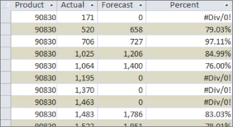
Figure 13.10 The errors shown in the results are due to the fact that some revenues are being divided by zeros.
Although this seems like a fairly benign issue, in a more complex, multilayered analytical process, these errors could compromise the integrity of your data analysis. To avoid these errors, you can perform a conditional analysis on your dataset using the IIf function, evaluating the Forecast field for each record before performing the calculation. If the forecast is zero, you'll bypass the calculation and simply return a value of zero. If the forecast is not zero, you'll perform the calculation to get the correct value. The IIf function would look like this:
IIf([Forecast]=0,0,[Actual]/[Forecast])Figure 13.11 demonstrates how this IIf function is put into action.
![Snipped image of a query in Design view with BranchForecasts table and a query grid listing Field inputs Product, Actual, Forecast, and Percent: IIf([Forecast]=0,0,[Actual]/[Forecast]).](http://images-20200215.ebookreading.net/22/4/4/9781119086543/9781119086543__access-2016-bible__9781119086543__images__c13f011.jpg)
Figure 13.11 This IIf function enables you to test for forecasts with a value of zero and bypass them when performing your calculation.
As you can see in Figure 13.12, the errors have been avoided.
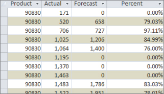
Figure 13.12 The IIf function helped you avoid the division by zero errors.
Saving time with IIf
You can also use the IIf function to save steps in your analytical processes and, ultimately, save time. For example, imagine that you need to tag customers in a lead list as either large customers or small customers, based on their dollar potential. You decide that you'll update the MyTest field in your dataset with “LARGE” or “SMALL” based on the revenue potential of the customer.
Without the IIf function, you would have to run the two update queries shown in Figures 13.13 and 13.14 to accomplish this task.

Figure 13.13 This query will update the MyTest field to tag all customers that have a revenue potential at or above $10,000 with the word “LARGE.”
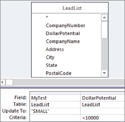
Figure 13.14 This query will update the MyTest field to tag all customers that have a revenue potential less than $10,000 with the word “SMALL.”
Will the queries in Figures 13.13 and 13.14 do the job? Yes. However, you could accomplish the same task with one query using the IIf function.
The update query shown in Figure 13.15 illustrates how you can use an IIf function as the update expression.
![Snipped image of a query in Design view with LeadList table and a query grid listing Update To input IIf([DollarPotential]>=10000, “LARGE”, “SMALL”).](http://images-20200215.ebookreading.net/22/4/4/9781119086543/9781119086543__access-2016-bible__9781119086543__images__c13f015.jpg)
Figure 13.15 You can accomplish the same task in one query using the IIf function.
Take a moment and look at the IIf function being used as the update expression.
IIf([DollarPotential]>=10000,"LARGE","SMALL")This function tells Access to evaluate the DollarPotential field of each record. If the DollarPotential field is greater than or equal to 10,000, use the word “LARGE” as the update value; if not, use the word “SMALL.”
Nesting IIf functions for multiple conditions
Sometimes the condition you need to test for is too complex to be handled by a basic IF…THEN…ELSE structure. In such cases, you can use nested IIf functions—that is, IIf functions that are embedded in other IIf functions. Consider the following example:
IIf([VALUE]>100,"A",IIf([VALUE]<100,"C","B"))This function will check to see if VALUE is greater than 100. If it is, then "A" is returned; if not (else), a second IIf function is triggered. The second IIf function will check to see if VALUE is less than 100. If yes, then "C" is returned; if not (else), "B" is returned.
The idea here is that because an IIf function results in a true or false answer, you can expand your condition by setting the false expression to another IIf function instead of to a hard-coded value. This triggers another evaluation. There is no limit to the number of nested IIf functions you can use.
Using IIf functions to create crosstab analyses
Many seasoned analysts use the IIf function to create custom crosstab analyses in lieu of using a crosstab query. Among the many advantages of creating crosstab analyses without a crosstab query is the ability to categorize and group otherwise unrelated data items.
In the example shown in Figure 13.16, you're returning the number of account managers hired before and after 2014. Categorizations this specific would not be possible with a crosstab query.
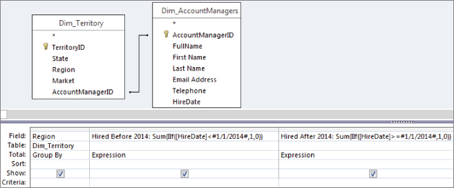
Figure 13.16 This query demonstrates how to create a crosstab analysis without using a crosstab query.
The result, shown in Figure 13.17, is every bit as clean and user-friendly as the results would be from a crosstab query.
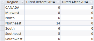
Figure 13.17 The resulting dataset gives you a clean crosstab-style view of your data.
Another advantage of creating crosstab analyses without a crosstab query is the ability to include more than one calculation in your crosstab report. For example, Figure 13.18 illustrates a query where the sum of units and revenue will be returned in crosstab format.

Figure 13.18 Creating crosstab-style reports using the IIf function allows you to calculate more than one value.
As you can see in Figure 13.19, the resulting dataset provides a great deal of information in an easy-to-read format. Because a standard crosstab query does not allow more than one value calculation (in this case, units and revenue are values), this particular view would not be possible with a standard crosstab query.
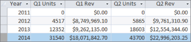
Figure 13.19 This analysis would be impossible to create in a standard crosstab query, where multiple calculations are not allowed.
The Switch function
The Switch function enables you to evaluate a list of expressions and return the value associated with the expression determined to be true. To use the Switch function, you must provide a minimum of one expression and one value.
Switch(Expression, Value)Expression(required): The expression you want to evaluateValue(required): The value to return if the expression is true
The power of the Switch function comes in evaluating multiple expressions at one time and determining which one is true. To evaluate multiple expressions, simply add another Expression and Value to the function, as follows:
Switch(Expression1, Value1, Expression2, Value2, Expression3, Value3)When executed, this Switch function evaluates each expression in turn. If an expression evaluates to true, the value that follows that expression is returned. If more than one expression is true, the value for the first true expression is returned (and the others are ignored). Keep in mind that there is no limit to the number of expressions you can evaluate with a Switch function.
Comparing the IIf and Switch functions
Although the IIf function is a versatile tool that can handle most conditional analyses, the fact is that the IIf function has a fixed number of arguments that limits it to a basic IF…THEN…ELSE structure. This limitation makes it difficult to evaluate complex conditions without using nested IIf functions. Although there is nothing wrong with nesting IIf functions, there are analyses in which the numbers of conditions that need to be evaluated make building a nested IIf impractical at best.
To illustrate this point, consider this scenario. It's common practice to classify customers into groups based on annual revenue or how much they spend with your company. Imagine that your organization has a policy of classifying customers into four groups: A, B, C, and D (see Table 13.1).
Table 13.1 Customer Classifications
| Annual Revenue | Customer Classification |
| >= $10,000 | A |
| >=5,000 but < $10,000 | B |
| >=$1,000 but < $5,000 | C |
| <$1,000 | D |
You've been asked to classify the customers in the TransactionMaster table, based on each customer's sales transactions. You can actually do this using either the IIf function or the Switch function.
The problem with using the IIf function is that this situation calls for some hefty nesting. That is, you'll have to use IIf expressions within other IIf expressions to handle the easy layer of possible conditions. Here's how the expression would look if you opted to use the IIf function:
IIf([REV]>=10000,"A",IIf([REV]>=5000 And [REV]<10000,"B",
IIf([REV]>1000 And [REV]<5000,"C","D")))
As you can see, not only is it difficult to determine what's going on here, but this is so convoluted that the chances of making a syntax or logic error are high.
In contrast to the preceding nested IIf function, the following Switch function is rather straightforward:
Switch([REV]<1000,"D",[REV]<5000,"C",[REV]<10000,"B",True,"A")This function tells Access to return a value of "D" if REV is less than 1000. If REV is less than 5000, a value of "C" is returned. If REV is less than 10000, "B" is returned. If all else fails, use "A". Figure 13.20 demonstrates how you would use this function in a query.

Figure 13.20 Using the Switch function is sometimes more practical than using nested IIf functions. This query will classify customers by how much they spend.
When you run the query, you'll see the resulting dataset shown in Figure 13.21.

Figure 13.21 Each customer is conditionally tagged with a group designation based on annual revenue.