
70 ◾ Advances in Communications-Based Train Control Systems
where:
k =
1,2,3,
...
nj
N,{1,2,...,
}∈
Based on the measurement data, we observe that most transitions within a
Markov chain are between adjacent states. erefore, we assume that each
state can only transit to the adjacent states, which means
p
nj,
0=
, if
||
nj
− >1
.
With the denition, we can dene a state transition probability matrix
P
with
elements
p
nj
,
.
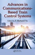
(b)
Shark-fin antenna
(a)
(c)
(d)
Figure4.3 (a) Tunnel where we performed the measurements in Beijing Subway
Changping Line. (b) Shark-n antenna located on the measurement vehicle.
(c)Yagi antenna. (d) AP set on the wall.

Modeling of the Wireless Channels in Underground Tunnels ◾ 71
Due to the eect of large-scale fading, the amplitude of SNR depends on the
distance between the transmitter and the receiver. It is obvious that the SNR is
usually high when the receiver is close to the transmitter, whereas it is low when
the receiver is far away from the transmitter. As a result, the transition prob-
ability from the high channel state to the low channel state is dierent when the
receiver is near or far away from the transmitter, which means that the Markov
state transition probability is related to the location of the receiver. erefore,
only one state transition probability matrix, which is independent of the location
of the receiver, may not accurately model the tunnel channels. us, we divide
the tunnel into
L
intervals and one state transition probability matrix is generated
for each interval. Specically,
P
l
lL
,{1,2,...,
}
∈
is the state transition probability
matrix corresponding to the l th interval, and the relationship between the tran-
sition probability and the location of the receiver can be built. en,
p
nj
l
,
is the
state transition probability from state
s
n
to state
s
j
in the l th interval. And the
state
n
and the state
j
in the l th interval are denoted as
s
n
l
and
s
j
l
, respectively.
Table 4.1 Notions of Symbols
γ
k
The channel state in time slot k
N The number of SNR levels
L The number of distance intervals
Γ
n
The threshold of the nth level of SNR
s
n
The channel state n
p
n,
j
The transition probability from state s
j
to state s
n
P
l
The transition probability matrix in the l th interval
s
n
l
The channel state n in the l th interval
p
nj
l
,
The transition probability from state
s
j
l
to state
n
a
n
l
The number of times state
s
n
l
appears
a
nj
l
,
The number of times that states
s
j
l
transits to state
s
n
l
Γ
n
The quantized value of SNR in the range
(ΓΓ
nn−
1
)
L
m
The maximized value of the likelihood function
η
The number of parameters of the statistical model
n
s
The number of channel samples

72 ◾ Advances in Communications-Based Train Control Systems
Consequently, the state probabilities and the state transition probabilities can be
dened as follows:
pP s
pP
ss
pnj
n
l
r
l
k
l
n
l
nj
l
r
l
k
l
n
l
k
l
j
l
nj
l
==
===
=−
+
{}
{}
0,
,1
,
γ
γγ|
|if || >1
1, {1,2,3,..., }
1
,
j
N
nj
l
pn N
=
∑
=∀∈
(4.2)
where:
p
n
l
is the probability of being in state
n
in the
l
th interval
γ
k
l
is the SNR level in time slot
k
in the
l
th interval
Based on the measurement results, we can determine the value of the state prob-
ability
p
n
l
and the state transition probability
p
nj
l
,
:
p
as
as
n
l
n
l
k
l
n
l
n
l
k
l
n
l
n
N
=
=
=
=
∑
{}
{}
1
γ
γ
(4.3)
where
as
n
l
k
l
n
l
{}
γ=
is the number of times state
s
n
appears in the
l
th interval.
p
ass
ass
nj
l
nj
l
k
l
n
l
k
l
j
l
nj
l
k
l
n
l
k
l
j
l
j
N
,
,1
,1
1
{}
{}
=
==
==
+
+
=
γγ
γγ
|
|
∑∑
(4.4)
where
ass
nj
l
k
l
n
l
k
l
j
l
,1
{}γγ
+
==
| is the number of times that state
j
transits to state
n
in the
l
th interval.
4.3.2 Determine the SNR-Level Thresholds
of the FSMC Model
Determining the thresholds of SNR levels is the key factor that aects the accuracy
of the FSMC model. ere are many methods to select the SNR-level boundaries,
among which the equiprobable partition method is frequently used in previous
works [9,10]. As nonuniform amplitude partitioning can be useful to obtain more
accurate estimates of system performance measures [15], we choose the Lloyd–Max
technique [14] instead of the equiprobable method to partition the amplitude of
SNR in this chapter. Lloyd–Max is an optimized quantizer, which can decrease the
distortion of scalar quantization.

Modeling of the Wireless Channels in Underground Tunnels ◾ 73
First, a distortion function D is dened as follows:
Dfp
n
N
n
n
n
=−
∑
∫
−
=1
1
()()
Γ
Γ
Γ
γγγd
(4.5)
where:
Γ
n
is the quantized value of SNR whose amplitude is in the range (
ΓΓ
nn
−1
)
fx()
is the error criterion function
p
()γ
is the probability distribution function of SNR
e distortion function can be minimized through optimally selecting
Γ
n
and
Γ
n
.
en, the necessary conditions for minimum distortion are obtained by dif-
ferentiating D with respect to
Γ
n
and
Γ
n
. e result of this minimization is a pair
of equations [16]:
ff
nn
()
()
1
ΓΓ
ΓΓ
−= −
+
nn
(4.6)
′
−=
−
∫
fp
n
n
n
()() 0
1
Γ
Γ
Γ
γγγd
(4.7)
e error criterion function
fx()
is often taken as
x
2
[16]. As a result, Equations4.6
and 4.7 become
Γ
ΓΓ
n
nn
=
+
+
1
2
(4.8)
()() 0
1
Γ
Γ
Γ
n
n
n
p
−=
−
∫
γγγd
(4.9)
As mentioned above, we partition the amplitude of SNR into
N
levels, and there
are
N +1
corresponding thresholds
{,
0,1,2,3,...
,}Γ
n
nN=
. Generally, the rst and
last thresholds are known, which are denoted by the minimum and maximum
measurement values of SNR, respectively. Furthermore, the Lloyd–Max algorithm
is used to divide
2
r
levels, which means
Nr
r
= =2, 1,2,3,
...
, and
N
is an even num-
ber. As a result, as
Γ
0
and
Γ
N
are known,
Γ
N
2
can be obtained from Equation 4.9. en,
Γ
N
4
and
Γ
34
N
can also be calculated according to the new variable
Γ
N
2
, when
r
is
larger than 2. With the process being repeated, all elements of
{}Γ
n
can be obtained
as follows:

74 ◾ Advances in Communications-Based Train Control Systems
Γ
Γ
Γ
ba
a
b
p
ba bNa
+
−
=
∈∈
∫
2
() 0
>{2,3,...,}, {1,2,3
γγγd
and,,...,1}N−
(4.10)
where:
p
()γ
is the probability distribution function of SNR
According to the calculated
{}Γ
n
, combined with Equations 4.8 and 4.9, we can
update the value of
{}Γ
n
until the value of
D
is the minimum, and the optimal
thresholds of the SNR levels can be obtained. As
p
()γ
is still unknown, we should
discuss the distribution of SNR in Section 4.3.3 according to the real eld measure-
ment data, which is the last step to obtain the thresholds of SNR levels.
4.3.3 Determine the Distribution of SNR
Deriving the distribution of SNR is the crucial step of partitioning the levels of
SNR. In fact, there are some classic models to describe the distribution of signal
strength, such as Rice, Rayleigh, and Nakagami, and then the corresponding mod-
els of SNR can also be obtained [17]. We rst derive the distribution of the signal
strength in order to determine the distribution model of SNR. According to [17]
and [18], voltage/meter (v/m) is usually used when studying the distribution of
small-scale fading. erefore, we convert dBm to the linear unit v/m following [19].
e Akaike information criterion (AIC) is often used to get the approximate
distribution model of the signal strength [20]. It is a measure of the relative good-
ness of t of a statistical model. It was developed by Hirotsugu Akaike, under the
name of an information criterion, and was rst published in 1974. e general case
of AIC is
AIC
=− +22
lnL
m
η
(4.11)
where:
η
is the number of parameters of the statistical model
L
m
is the maximized value of the likelihood function for the estimated model
In fact, according to the relationship of
η
and the number of samples
n
s
, AIC needs
to be changed to AIC with a correction (AICc) when
n
s
/<
40η
[20].
AICc AIC=+
+
−−
2( 1)
1
ηη
ηn
s
(4.12)
In this chapter, AICc is adopted to estimate the model of the signal strength
distribution instead of the classic AIC. In practice, one can compute AICc for each
..................Content has been hidden....................
You can't read the all page of ebook, please click here login for view all page.