Cognitive Control for CBTC Systems ◾ 233
communication delay, the back train has to brake in order to keep safe with the decel-
eration calculated by the ATO. As a result, we dene
C
c
as
AA
cb
,0,
[]
, where
A
c
is the
constant acceleration and
A
b
is the braking deceleration. After the ATO processes the
state vector
y
k
, the
x
k
c
is obtained to determine the relationship between the state of
the current train and the state of the front train. As the optimal train operation prole
is piecewise, we employ logical operations on the elements of
x
k
c
and fx
k
c
()
as follows:
fx
xxxxxx
xx xxx
k
c
kk kkkk
kk kkk
()=
[( )]
()(
122314
12 323
∧∨ ∧∧
∧∧¬∧¬
∧∧∧
∧∨¬
xx
xx x
kk
kk k
14
23 1
)
()
(10.29)
where:
xxxxx
k
c
kkkk
=[,,,]
1234
∧
is the logical
AND
∨
is the logical OR
is the logical XOR
¬
is
the logical NOT
As a result, according to the relationship between the states of two trains and some
constant parameters of the optimal train operation prole, ATO can determine the
acceleration of the train at each communication cycle.
10.5.3 Parameters of the Wireless Channel
According to the measurement results in Beijing Yizhuang Line, we derive the state
transition probability for each interval. e FSMC model is built with four states
and the
5m
distance interval. Figure 10.7 shows the measurement scenario.
According to the measurement results, one of the channel state transition matri-
ces is
P =
0.91 0.08
00
0.041 0.86 0.09 0
0 0.024 0.85 0.11
000.023 0.97
which shows the channel characteristics at the location 35–40m.
10.5.4 Simulation Results and Discussions
In this section, simulation results are presented and discussed. First of all, we pres-
ent the train control performance improvement. Next, the hando performance is
discussed. In addition, we show that the proposed cognitive control approach can
increase the reliability of train–ground communication, which is also an important
parameter for CBTC systems.

234 ◾ Advances in Communications-Based Train Control Systems
We implement the simulations using MATLAB. As mentioned earlier, we
get the channel state probability through real eld measurements. In our simula-
tion scenarios, there are two stations and the distance is
2256m
, which is the real
value of the distance between Tongji Nan and Jinghai stations in Beijing Subway
Yizhuang Line, and the regulated trip time is
150s
. According to the deployment of
wayside APs, the length of interval between two adjacent APs is
400m
. As a result,
there are six APs between these two stations. In the simulations, there are two
trains. e headway is rst set to
15s
, which means that the second train departs
from the starting station
15s
after the rst train leaves. e headway of
90s
is also
considered in the simulations. e parameters related to the dynamic model and
the wireless channel model are illustrated in Table 10.1.
(b)
Shark-fin antenna
(a)
(c)
(d)
Figure10.7 (a) Tunnel where we performed the measurements. (b) Shark-n
antenna located on the measurement vehicle. (c) Yagi antenna. (d)AP set on the
wall.

Cognitive Control for CBTC Systems ◾ 235
ere are three policies in our simulations for comparisons: the proposed cog-
nitive control policy, the semi-Markov decision process (SMDP) policy, and the
greedy policy. Based on the Markov property of state transition process, it is pos-
sible to model the problem considered in this chapter as an SMDP [29] and derive
the SMDP policy. In the greedy policy, if there is one AP whose signal strength
is higher than the current associated AP, the MS switches to the AP with higher
signal strength. In other words, the greedy policy always makes decisions based on
the immediate reward, not the long-term reward.
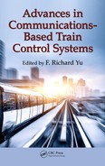
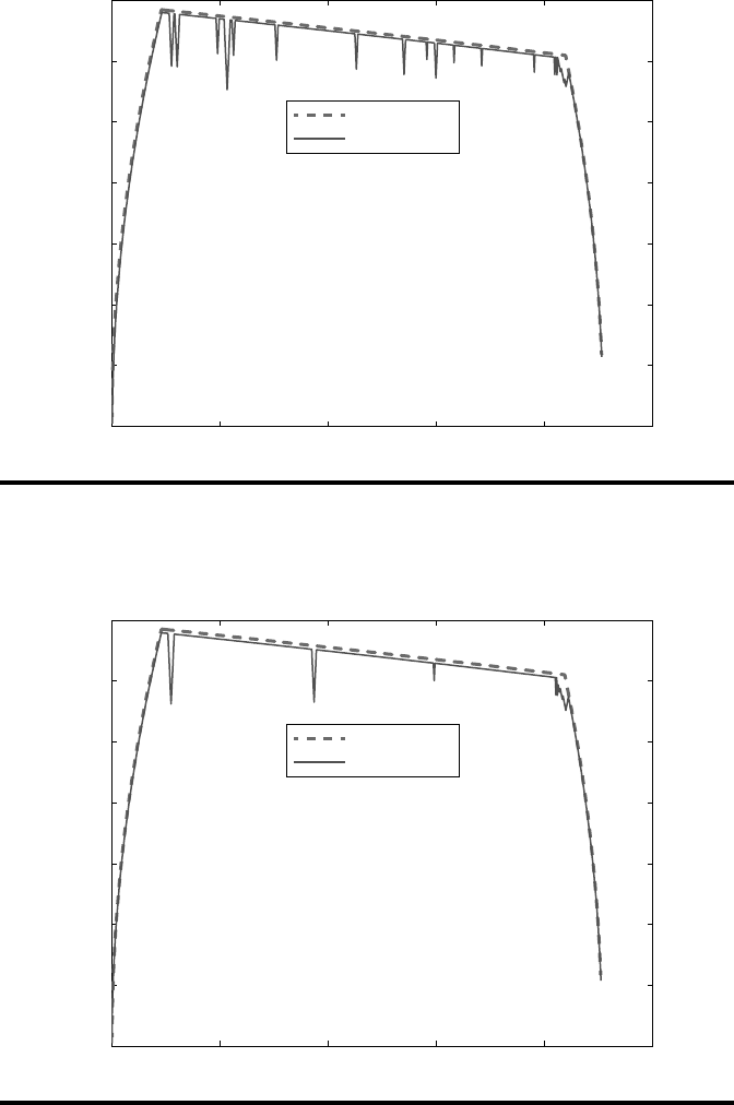
First of all, we compare the cost function under dierent policies. As shown in
Figure 10.8, the
x
-axis represents the index of the communication cycle and the
y
-axis
is the cost in each communication cycle. Under the greedy and SMDP policies, the
cost increases sharply in some communication cycles, which means that the informa-
tion gap becomes larger due to the long hando latency. Obviously, the SMDP policy
can bring better performance and less cost with less peaks compared with the greedy
policy. However, the cost under the proposed cognitive control policy is a smooth
curve, which means that no long hando latency happens. Figure 10.8 indicates
that the cognitive control can help the MS to make the optimal hando decision
through minimizing the information gap, which can decrease the cost of train con-
trol including the tracking errors and energy consumption.
e travel trajectories of these two trains under dierent policies are shown in
Figures 10.9 through 10.11, where the
x
-axis is the position of trains and the
y
-axis
is the corresponding velocity of trains. Under dierent policies, the current (back)
train follows dierent travel curves. When the greedy policy and the SMDP policy
are used, the train will be o the preset running prole sometimes due to the large
information gap. e hando latency enlarges the information gap, and the current
train has to slow down in order to keep the safe distance. Next, when the latest MA
is received by the train and the information gap is eliminated, the current train has
to speed up to reach the optimal running prole. As there are frequent accelera-
tions and decelerations, it can cause much more energy consumption. By contrast,
as shown in Figure 10.11, the current train with the cognitive control policy can be
very close to the optimal running prole, which means improved passenger com-
fort and energy saving in the proposed scheme.
We also consider the case when the headway is 90s, which is the standard
headway used in Beijing Yizhuang Line. From Figures 10.12 through 10.14,
Table 10.1 Availability under Different Policies
Policy Availability (A
av
) Unavailability (1 – A
av
)
Cognitive control 0.9978 2.2 × 10
–3
SMDP 0.9413 5.87 × 10
–2
Greedy 0.8833 1.167 × 10
–1

236 ◾ Advances in Communications-Based Train Control Systems
0 100 200 300 400 500 600 700 80
0
10
3
10
4
10
5
10
6
10
7
10
8
10
9
10
10
Index of communication cycle(a)
Cost
Cognitive control policy
Greedy policy
0 100 200 300 400 500600 70
0800
10
3
10
4
10
5
10
6
10
7
10
8
10
9
10
10
Index of communication cycle(b)
Cost
Cognitive control policy
SMDP policy
Figure10.8 (a) Cost function
J
at each communication cycle under the greedy
policy and the proposed cognitive control policy. (b) The cost function J at each com-
munication cycle under the SMDP policy, and the proposed cognitive control policy.
Cognitive Control for CBTC Systems ◾ 237
0 500 1000 1500 2000
2500
0
10
20
30
40
50
60
70
Distance (m)
Velocity (km/h)
Front train
Current train
Figure10.9 Train travel trajectory under the greedy policy (the headway is 15s).
Front train
Current train
0 500 1000 1500 2000
2500
0
10
20
30
40
50
60
70
Distance (m)
Velocity (km/h)
Figure10.10 Train travel trajectory under the SMDP policy (the headway is 15s).
..................Content has been hidden....................
You can't read the all page of ebook, please click here login for view all page.