120 ◾ Advances in Communications-Based Train Control Systems
latency impact on CBTC eciency when hando happens. e communication
latency impact when hando does not happen is ignored. is is because the com-
munication latency under this circumstance is only several milliseconds, and it is
less than the communication period. In the simulation scenario, there are three
trains traveling between two stations. e wayside base stations are deployed along
the railway line with an average distance of
600m
between two successive base sta-
tions. e three trains depart from the station A successively with
16s
interval and
stop at the station B. e communication period is
200ms
, the start acceleration
is
1/
2
ms
, the deceleration that denes the ATP service braking curve is set to be
1.2
/
2
ms, the rail limited speed is
80
/km
s
, the train length is
100m
, and the system
response time is
100ms
.
Based on the train and rail parameters, we rst calculate the travel time between
stations when the communication latency impact is not considered. e distances
between two stations are set to be
2000
,
3000
,
4000
,
5000
, and
6000m
, respec-
tively. Figure 7.2 shows the trip error between the third departed train and the rst
departed train when the hando communication latency is
2
,
4
, and
6s
. As shown
in the gure, the communication latency caused by hando would lead to second
trip time error. e ATS subsystem needs to adjust the timetable to make up the
wasted time in the last station sections, which severely decreases the utilization
of whole railway network infrastructure. In order to mitigate these impacts, we
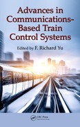
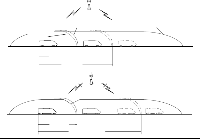
ATP emergency
braking curve
ATO guidance
trajectory
(a)
(b)
Old MA
New MA
Old MA
Delayed new MA
Train 2Train 1Train 1
Train 2Train 1Train 1Train 1
ATP service braking
curve
Figure7.1 Impacts of wireless communications on CBTC efciency. (a) Without
communication latency. (b) With communication latency.

Novel Communications-Based Train Control System ◾ 121
propose a CBTC train–ground communication system with CoMP, which will be
presented in Section 7.2.2.
7.2.2 Proposed CBTC System with CoMP
e proposed CBTC system with CoMP is shown in Figure 7.3. Unlike the exist-
ing CBTC system, in the proposed system, a train can communicate with a cluster
of base stations (BS1–BS4) (e.g., clusters C1–C5 in Figure 7.3) simultaneously,
which is dierent from the current CBTC systems, where a train can only com-
municate with a single base station at any given time. When a base station fails, the
remaining base stations in the cluster can still guarantee the availability of train–
ground communications.
In the above system, as trains travel on the railway, the received SNR changes
rapidly. e communication latency will be a serious problem when the MT on
the train is in deep fading. In theory, CoMP communication can extend cell
coverage and increase capacity in wireless networks. However, because the chan-
nel state information from the involved base stations is needed in CoMP sys-
tems, practical systems that employ CoMP techniques suer from constraints
imposed by the backhaul network, which is used to exchange the channel state
information from the involved base stations. Backhaul networks are constrained
2000 2500 3000 3500 4000 4500 5000 5500
6000
0
1
2
3
4
5
6
7
8
9
Distance between stations (m)
Travel time error (s)
Communication latency = 6 s
Communication latency = 4 s
Communication latency = 2 s
Figure7.2 Trip error under different handoff communication latencies.

122 ◾ Advances in Communications-Based Train Control Systems
in capacity and introduce lost and/or outdated channel state information, which
will result in performance degradation of CoMP systems. erefore, we need to
decide whether or not to use CoMP considering the potential quality-of-service
(QoS) gain of CoMP and QoS degradation caused by the backhaul infrastruc-
ture latency.
More importantly, compared with CoMP-based commercial cellular systems,
handos happen quite frequently in CBTC systems. erefore, one of the criti-
cal issues in the system is the hando decision (i.e., when to perform hando)
problem. If the hando decision policy is not designed carefully, ping-pong eect
and long communication latency may occur, which will signicantly aect the
performance of a CBTC system. erefore, an ecient hando decision policy
is needed to decide at what time to trigger a hando and whether or not CoMP
communication should be used. In addition, due to the hando latency in the
system, it is also desirable to mitigate the impacts of hando latency on the sys-
tem control performance.
7.3 System Models
In this section, we describe the system models that will be used in our train control
performance optimization. We rst present the train control model. e commu-
nication channel model is described next.
Central scheduler
Backhaul network
BS1 BS2 BS3 BS4
C1 C2 C3
Train 1
C5C4
Figure7.3 Proposed CBTC system with CoMP.

Novel Communications-Based Train Control System ◾ 123
7.3.1 Train Control Model
Figure 7.4 presents the train control model used in the chapter. e ATP subsystem
rst receives the MA (that has the front train states) sent from the ZC through the
wireless link. It then calculates the braking curve for the received MA. e braking
command will be executed when the train velocity is greater than the target velocity
on the braking curve. Otherwise, the train is controlled by the ATO system. e
ATO subsystem gets train states (velocity, position, etc.) from the ATP subsystem.
It gives traction or braking command to bring the train to the guidance trajectory
after comparing the train travel trajectory with the optimized guidance trajectory.
According to the train dynamics, the train state space equation can be written
as [3]
qk qk vk T
uk
M
T
wk wk wk
M
T
vk
irw
()(()
()
1
2
() () ()
(1)
2
+1)
1
2
2
=+⋅+
−
++
+=
vvk
uk
M
T
wk wk wk
M
T
irw
()
() () () ()
+⋅−
++
(7.1)
where:
T
is the sampling rate, which depends on the communication period
qk()
is the train position at time
k
vk()
is the train velocity
M
is the train mass
wk
i
()
is the slope resistance
Braking
ATO ATP
Train dynamic model
x(k + 1) = Ax(k) + Bu(k) + Cw(k)
z(k) = C
o
x(k)
x
c
(k + 1) = A
c
x
c
(k) + B
c
y
c
(k)
u(k) = C
c
x
c
(k)
Traction
Disturbance
Front train states
obtained from wireless
link
Figure7.4 Train control model.
124 ◾ Advances in Communications-Based Train Control Systems
wk
r
()
is the curve resistance
w
w
k
()
is the wind resistance
uk
()
is the train control command from the train controller
CBTC systems use packet-based transmission of train control information.
Compared to traditional track-based train control systems, where the train
only reports its location to the ground equipment and receives the information
from ground equipment in specic places, in CBTC systems, the train sends
its location and receives the MA from ground ZC continuously. In real sys-
tem implementations, both information processing and transmission need time.
erefore, data packets are exchanged between the ground ZC and trains on a
poll-response basis with a typical cycle time, which is the communication period
in our chapter.
Equation 7.1 can be rewritten as
xk Ax kBuk Cw k(1)()(
)(
)
+= ++
(7.2)
where:
xk
qk vk() {()()}
=
is the state space
wk wk wk
wk
irw
() () ()
()=++
is the extra resistance acting on the train
e train dynamics model described in Equation 7.1 has been widely used in opti-
mal train control studies [13,14]. It is shown that the optimal control problem for
a train with a distributed mass on a track with a continuously varying gradient can
be replaced by an equivalent problem for a point mass train, and that any strategy
of continuous control can be approximated as closely as a strategy with discrete
control.
We assume that the train controller is linear time invariant in discrete time and
has the following state space model [3]:
xk Ax kByk
uk Cx k
cc
cc
cc
(1)= ()
()
()=()
++
(7.3)
where:
yk()
is the controller input, which includes the states of the two trains
xk
c
()
is the state of the controller
In this chapter, we use velocity tracking error as the state of the controller. Linear
controllers have been successfully used in train control systems. For example, in
[15], a linear controller is used in high-speed trains, where the commander of the
controller is linearly and invariantly proportional to system states. Moreover, in this
chapter, the SMDP-based optimization algorithm is not dependent on a specic
..................Content has been hidden....................
You can't read the all page of ebook, please click here login for view all page.