
Chapter 7. Alternative Computational Models
When people talk about the benefits of using DSLs, you often hear them say that they support a more declarative approach to programming. I confess to having a problem with the word “declarative”; it often seems to be used as a very broad brush. In general, however, declarative means “something other than imperative.”
Mainstream programming languages follow the imperative computational model. The imperative model defines computation through a sequence of steps: do this, do that, if (red) do the other. Conditionals and loops vary the steps, and steps can be grouped together into functions. Object-oriented languages add bundling together of data and process, as well as polymorphism—but are still grounded in an the imperative model.
The imperative model gets quite a bit of flak thrown at it, particularly from academics, but it has continued to be our fundamental computational model since the early days of computing. I think this is because it’s easy to understand: Sequences of actions are something that is straightforward to follow.
When we talk about ease of understanding, there are really two different kinds of understanding in play. The first is understanding the intent of the program—what are we trying to achieve with it. The second form of understanding is of the implementation—how the program works to satisfy the intent. The imperative programming model is particularly good with the latter: You can read the code and see what it’s doing. To get more details, you can step through with a debugger—the sequence of the statements in the source code corresponds exactly to what happens in the debugger.
Where the imperative approach doesn’t always work so well is in the understanding of intent. If the intent is a sequence of actions, fine; but often, our intentions aren’t best expressed that way. In these cases, it is often worth considering a different computational model.
I’ll start with a simple example. Often, you run into situations where you need to state the consequences for different combinations of conditions. A small example of this might be scoring points to assess car insurance, where you might see something like Figure 7.1.
Figure 7.1 A simple decision table for car insurance
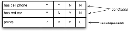
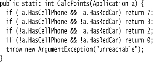
This kind of table is a common way for people to think about this kind of problem. If we turn this table into imperative C# code, we’d see something like this:
My normal style of writing Boolean conditions is rather more terse, something like this:
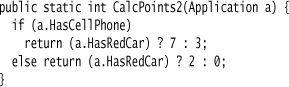
But in this case I prefer the first, longer way of writing it because the code corresponds more closely to the intent of the domain expert. The tabular nature of how she thinks about it is similar to the way the code is laid out.
There’s similarity between the table and the code, but they’re not quite the same. The imperative model forces the various if statements to be executed in a particular order, which isn’t implied by the decision table. This means that I’m adding an irrelevant implementation artifact to my representation of the table. For decision tables this isn’t a big deal, but it can matter for other alternative computational models.
A potentially more serious shortcoming of an imperative representation is that it removes some useful opportunities. One of the nice things about a decision table is that you can check it to ensure you don’t miss a permutation, or that you don’t accidentally repeat a permutation.
An alternative to using imperative code is to create a decision table abstraction and then configure it for this particular case. If I do that, I could represent this table with something like this:
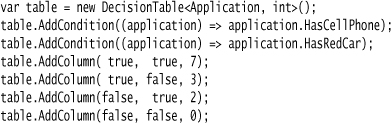
I now have a more faithful representation of the original decision table. I no longer specify the order of evaluating the conditions in the imperative code; that’s left to the insides of the decision table (this lack of ordering may be handy to exploit concurrency). More importantly, the decision table can check for a properly formed set of conditions and tell me if I’ve missed anything in my configuration. As a bonus, I shift my execution context from compile time to runtime and can thus change the rules without a recompile.
I call this style of representation an Adaptive Model. The term “adaptive object model” has been around for a while to describe how this is done as an OO model; take a look at writings by Joe Yoder and Ralph Johnson [Yoder and Johnson]. But you don’t need to use objects to do something like this—storing data structures that capture behavioral rules is common in databases too. Most decent OO models have objects contain behavior as well as data, but the defining thing about an Adaptive Model is that the behavior is largely defined by the instances of the model and how they are wired together. You cannot understand what behavior to expect without looking at the configuration of instances.
You don’t need a DSL to use an Adaptive Model. Indeed, DSLs and Adaptive Models are separate notions that can be used independently of each other. Even so, I suspect it should be obvious to you that Adaptive Models and DSLs go together like wine and cheese. Throughout this book, I’ve harped on and on about making the DSL parse build a Semantic Model. Often, this Semantic Model is an Adaptive Model that provides an alternative computational model for a part of a software system.
The big negative of using an Adaptive Model is that the behavior it defines is implicit; you can’t just look at the code to see what happens. On top of this, while the intention is usually easier to understand, the implementation is not. This becomes important when things go wrong and you need to debug. It’s often much harder to find faults with an Adaptive Model. I often hear people complain that they can’t find the program and can’t understand how it works. As a result, Adaptive Models have a reputation for being hard to maintain. Often, I hear about people taking months to figure out how it works. If they finally figure it out, the Adaptive Model can make them very productive, but before they do (and many people never do) it’s a nightmare.
This implementation comprehension problem with Adaptive Models is a real issue, and one that rightly deters many people from using them, despite the very real benefits you can get once you become comfortable with how they work. One of the benefits I see with DSLs is that they make it easier to understand how an Adaptive Model fits together and thus easier to program it. With a DSL, you can at least see the program. It doesn’t take away all the issues of understanding how the general Adaptive Model works, but being able to more clearly see the specific configuration can give you a significant leg up.
Alternative computational models are also one of the compelling reasons for using a DSL, which is why I’ve spent a big chunk of time on them in this book. If your problem can be easily expressed using imperative code, then a regular programming language works just fine. The key benefits of a DSL—greater productivity and communication with domain experts—really kick in when you are using an alternative computational model. Domain experts often think about their problems in a nonimperative way, such as via a decision table. An Adaptive Model allows you to capture their way of thinking more directly in a program, and the DSL allows you to communicate that representation more clearly to them (and yourself).
7.1 A Few Alternative Models
There are many possible computational models out there, and I’m not going to provide a comprehensive picture of them in this book. What I can do is provide a small sample of common ones. These will help you in the common cases, but I also hope they may spark you imagination to come up with specific computational models for your domain.
7.1.1 Decision Table
Since I’ve already mentioned Decision Tables, I might as well start with them. It’s a pretty simple form of an alternative computational model, but well suited to a DSL. Figure 7.2 is a relatively simple example.
Figure 7.2 A decision table for handling orders
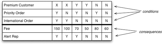
The table consists of a number of rows of conditions, followed by a number of rows of consequences. The semantics are straightforward; in this case, you take an order and check it against the conditions. One column of conditions should match, and then the consequences on that column apply. So, if we have a premium customer with a domestic, priority order, there’s a fee of $70 and we alert a representative to handle the order.
In this case, each condition is a Boolean condition, but more complicated decision tables can have other forms of conditions, such as numeric ranges.
Decision tables are particularly easy to follow for nonprogrammers, so they work well in communicating with domain experts. Their tabular nature makes them natural for editing in a spreadsheet, so this is one case of a DSL where direct editing by a domain expert is more likely than not.
7.1.2 Production Rule System
The general notion of modeling logic by dividing it up into rules, each of which has a condition and a consequent action, is a Production Rule System. Each rule can be specified individually in a style similar to a bunch of if-then statements in imperative code.
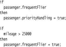
With a Production Rule System, we specify these rules in terms of their conditions and actions, but we leave it to the underlying system to execute them and tie them together. In the example I just showed, there is a link between the rules in that if the second rule is true (and thus “fired,” as it’s said in the local lingo), that may affect whether the first rule should be fired.
This characteristic, where firing some rules changes whether other rules should be fired, is called chaining, and is an important characteristic of a Production Rule System. Chaining allows you to write rules individually, without thinking of their broader consequences, and then let the system figure out those consequences.
This benefit is also a danger. A Production Rule System relies a lot on implicit logic, which can often do things that weren’t anticipated. Sometimes this unanticipated behavior can be beneficial, but sometimes it can be harmful, leading to an incorrect result. These errors are often precisely due to the fact that the writers of the rules haven’t taken into account how rules interact.
Problems due to implicit behavior are a common issue with alternative computational models. We are relatively used to the imperative model, but still make lots of mistakes with it. With alternative models, we are even more prone to problems because we often cannot reason easily about what will happen just by looking at the code. A bunch of rules embedded in a rule base will often produce surprising results, for good or ill. One consequence of this, which applies to most cases where you implement an alternative computational model, is that it’s important to produce a tracing mechanism so you can see what exactly happened on an execution of the model. With Production Rule System, this means the ability to record which rules fired and provide that record easily when required, so that a puzzled user or programmer can see the chain of rules that led to an unexpected conclusion.
Production Rule Systems have been around for a long time, and there are many products that implement them and provide sophisticated tools for capturing and executing the rules. Despite this, it can still be useful to write a small Production Rule System within your own code. Like any case where you roll your own alternative computational model, you can usually get away with something relatively simple when you do it at a small scale with a particular domain in mind.
Although chaining is certainly an important part of a Production Rule System, it actually isn’t mandatory. Sometimes it’s useful to write a Production Rule System without chaining, a good example for which is a set of validation rules. With validation, you are often just capturing a bunch of conditions where the action is raising an error. Although you don’t need chaining, thinking of the behavior as a set of independent rules is still useful.
You can argue that a Decision Table is a form of Production Rule System where each column in the Decision Table corresponds to a single rule. While this is true, I think it misses the point. With a Production Rule System, you focus on the behavior one rule at a time; with a Decision Table, you focus on the entire table. That shift in thinking is an essential part of the two models, making them different mental tools.
7.1.3 State Machine
I opened this book with another popular alternative computational model—the State Machine. A State Machine models the behavior of an object by dividing it into a set of states and triggering behavior with events so that, depending on the state the object is in, each event leads to a transition to a different state.
Figure 7.3 indicates that we can cancel an order in the collecting and paid states, either of which will transition the order to the cancelled state.
Figure 7.3 A UML state machine diagram for an order
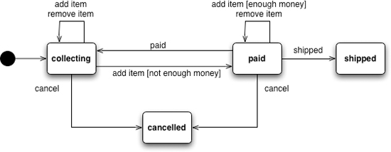
The State Machine has the core elements of states, events, and transitions, but there are a lot of variations that build on that basic structure. Variations particularly appear in how the State Machine initiates actions. A State Machine is a common choice because many systems can be thought of as reacting to events by going through a series of states.
7.1.4 Dependency Network
One of the most familiar alternative models in the daily work of software developers is the Dependency Network. It’s familiar because this model underpins build tools such as Make, Ant, and their derivatives. In this model, we look at the tasks that need to be done and capture the prerequisites for each task. For example, the task to run tests may have the compile and load data tasks as prerequisites, both of which have the generate code task as a prerequisite. With these dependencies stated, we can then invoke the test task, and the system figures out which other tasks need to be done and in what order. Furthermore, even though the generate code task appears twice in the list (because it’s listed twice as a prerequisite) the system knows it only needs to run it once.
Figure 7.4 A possible dependency network for building software
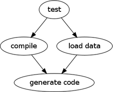
A Dependency Network is thus a good choice when you have computationally expensive tasks with dependencies between them.
7.1.5 Choosing a Model
I find it hard to come up with particular guidelines as to when to choose a particular computational model. It really all boils down to a sense that the computational model fits the way you think about your problem. The best way to determine whether it does fit is to try it out. Initially, just try it on paper by describing behaviors using simple text and diagrams. If a model seems to pass that simple desk check, then it’s worth building it, perhaps as a prototype, to see how it works in action. My feeling is that the key thing is to get the Semantic Model working properly, but it may help to use a simple DSL to help in this process. I’d put more effort into tuning the model first, however, before getting a very readable DSL. Once you have a reasonable Semantic Model in place, it’s relatively easy to experiment with different DSLs to drive it.
There are many more alternative computational models than these. If I had more time to spend on this book, I’d like to spend it on writing up more of them. It strikes me that a book of computational models would be a good book for somebody to write.