Modeling and Processing with Quadric Surfaces
Quadric surfaces, or quadrics, are surfaces defined by algebraic equations of degree two. We will discuss mainly quadrics in 3D space, though quadrics in higher dimensions are also of certain interest to CAGD. In this chapter the following topics concerning quadrics will be discussed.
31.1 DEFINITION AND CLASSIFICATIONS
In this section we will define quadrics and discuss their classifications under different groups of transformations, i.e., Euclidean, affine, and projective transformations [41].
31.1.1 Definition
A quadric is defined by a homogeneous quadratic equation F(x, y, z, w) = 0, where (x, y, z, w) are the homogeneous coordinates of a point in 3D space, with the corresponding affine coordinates (x/w,y/w, z/w) for a finite point, i.e., w ≠ 0. The matrix representation of a quadric surface is given by
where X = (x, y, z, w)T is the column vector of coordinates and M is a 4 × 4 real symmetric matrix.
The geometric degeneracy of a quadric is determined by the rank of M. If the rank of M is 4, then the quadric is called nondegenerate or proper. If the rank of M is less than 4, then the quadric is called singular. When the rank of M is 3, the quadric is singular but irreducible, and is therefore called properly degenerate. The properly degenerate quadrics are cones and cylinders. When the rank of M is 1 or 2, the quadric degenerates to a pair of planes. The case of rank(M) = 0 is trivial and will not be considered. Since only real points on a quadric surface are of interest in practical applications, we assume, without loss of generality, that the entries of M are real numbers and that M is indefinite, i.e., there exist real points X0and X1such that X0TMX0> 0 and X1T MX1< 0. Note that this assumption excludes those quadrics that are not real surfaces.
31.1.2 Euclidean classification
A Euclidean transformation is represented by
where O is a 3 × 3 orthogonal matrix with det(O) = 1, and B is a 3D translation vector. A Euclidean transformation X′ = UX transforms a quadric XT MX = 0 to a quadric XT(U−T MU−1)X ′ = 0. Under Euclidean transformations an irreducible quadric can be converted to one of the following nine canonical forms.
The first three of the above are called central quadrics. Properly degenerate quadrics:
Reducing a quadric surface to one of the above canonical forms by a Euclidean transformation is useful in analyzing quadrics, since this means that only one routine is needed to process each of the canonical forms and it is therefore not necessary to cope with an arbitrary quadratic form.
The fact that any quadric can be converted by a Euclidean transformation to one of these simple forms implies the existence of a local orthogonal coordinate system in which that form is assumed. In the case of a central quadric the coordinate axes of this coordinate system are the principal axes of the quadric. Denote
In this case the vectors of the three axes of a central quadric XT MX = 0 are the eigenvectors of ![]() 3×3, and the center of the quadric is given by -
3×3, and the center of the quadric is given by -![]() −1m, in Cartesian coordinates. Reducing a quadric surface in E3 to a canonical form is closely related to the orthogonal reduction of a quadratic form to a diagonal form. The reader is referred to [29] for a discussion of the reduction procedure, as well as a general discussion about the classification of quadrics under different transformation groups.
−1m, in Cartesian coordinates. Reducing a quadric surface in E3 to a canonical form is closely related to the orthogonal reduction of a quadratic form to a diagonal form. The reader is referred to [29] for a discussion of the reduction procedure, as well as a general discussion about the classification of quadrics under different transformation groups.
31.1.3 Affine classification
An affine transformation is represented by
where A is a 3 × 3 nonsingular matrix and B is a 3D translation vector. Under affine transformations an irreducible quadric can be converted into one of the following nine canonical forms. Since more general transformations are allowed in affine space than in Euclidean space, the coefficients in the following affine canonical forms are less arbitrary than those in the Euclidean canonical forms.
Note that the principal axes of a central quadric are not, in general, mapped to the principal axes of the transformed quadric under an affine transformation. However, the center of a central quadric is mapped to the center of the transformed quadric by an affine transformation.
31.1.4 Projective classification
A real projective transformation in 3D is given by X′ = AX, where A is any real 4×4 nonsingular matrix. A quadric is mapped to a quadric under a projective transformation and the rank of the coefficient matrix is not changed. Any irreducible quadric can be transformed projectively to one of the following three canonical forms:
Other commonly used canonical forms for the doubly ruled quadric and the cone under projective transformations are the hyperbolic paraboloid xy - zw = 0 and the cylinder x2 + y2- w2 = 0, respectively.
Any of the affine canonical forms of quadrics can be obtained from one of the above three projective canonical forms by appropriately specifying an ideal plane for an affine realization of projective space. The affine views of quadrics in projective space are discussed in [11].
31.2 PARAMETRIC REPRESENTATION
For reasons of computational efficiency, rational or polynomial representations of curves and surfaces are preferred in CAGD because of their simple analytical properties. So one reason why quadrics are widely used in CAGD is that all quadrics have rational parameterizations of degree two. In this section we shall discuss the rational quadratic parameterization of a whole quadric surface and of a surface patch on a quadric.
31.2.1 Global rational parameterization
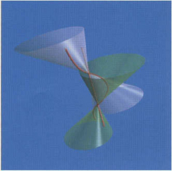
A simple way to derive a rational quadratic parameterization of a quadric is to use a stereographic projection of the quadric to establish a birational mapping between points on a plane and points on the quadric [41],[43]. See Figure 31.1. Let X0be a point on quadric S: XT AX= 0. Let B0T X= 0 be a plane not passing through X0. When S is a cone or cylinder, X0is assumed not to be the singular point of S. We will consider the projection that maps points on S through X0to points on plane BT0X = 0.
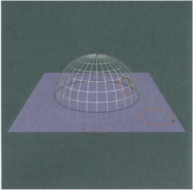
Let T = (x, y, z, w)T be a variable point on plane BT0X = 0, and let (r, s, t) be a projective coordinate system on BT0X = 0. Then there is a 4 × 3 matrix M such thatT = M(r, s, t)T, and T or (r, s, t) is called a parameter point. Let PT(u, v) = uX0+ vT be the line determined by X0and T. By Bézout’s theorem, there are two points of intersection between S and line PT(u, v) unless PT(u, v) is contained in S, and one of these two intersections is X0. The exception occurs for the generators of S at X0, i.e., the straight lines on S that pass through X0. Point X0is called the center of projection for the projection induced by the line PT(u, v) from plane BT0X = 0 to quadric XT AX = 0. Substituting PT(u, v) for X in XT AX = 0, the parameter pair corresponding to the other intersection is found to be u: v = TT AT: (-2XT0AT). Hence, the other intersection is
This is a faithful rational quadratic parameterization of S; a faithful parameterization is one that establishes a one-to-one correspondence between all points on the parametric plane and all points on the surface, with the usual exception of points on a finite number of curves on the surface.
Using the above procedure we obtain the following rational quadratic parameterization of the unit sphere S2: x2 + y2 + z2- w2 = 0,
with the center of projection at the north pole X0 = (0, 0, 1, 1) and projection plane z = 0. Here the homogeneous parameters (r, s, t) are identified with the homogeneous coordinates (x, y, w) in plane z = 0. (See Figure 31.1.) This is the standard stereographic projection of S2, which is circle-preserving.
A parametric rational quadratic surface is, in general, a quartic algebraic surface, but degenerates to a quadric in special cases [11]. A rational quadratic surface whose algebraic degree is higher than two is called a Steiner surface[37]. Steiner surfaces behave quite differently from rational quadratic curves, which are always conics. It is known from algebraic geometry [7] that the algebraic degree of a surface with a faithful rational quadratic parameterization is 4 - p, where p is the number of base points; a base point of a rational surface P(r, s, t) = (x(r, x, t), y(r, s, t), z(r, s, t), w(r, s, t)) is a parameter point (r0, s0, t0) ≠ (0, 0, 0) such that P(r0, s0, t0) = (0, 0, 0, 0). It follows that a faithful rational quadratic parameterization of a quadric has two base points. These two base points are distinct if and only if the quadric is nondegenerate [43].
The following properties of rational quadratic parameterizations of a quadric are proved elsewhere [43]. Two parameterizations derived using the above procedure with the same center of projection, but possibly with different projection planes, are related by a rational linear reparameterization; however, two parameterizations derived with two different centers of projection are related by a rational quadratic reparameterization, which is a 2D Cremona transformation [38]; a Cremona transformation is a birational transformation from plane to plane.
Any faithful rational parameterization of a quadric can be obtained using a stereo-graphic projection; but not all rational quadratic parameterizations are faithful. The following is an example of an unfaithful parameterization of the cone x2 + y2- z2 = 0:
It is unfaithful because, clearly, (r, s, t) and (r, s, -t) yield the same point on the cone. Unfaithful parameterizations can exist only for cones and cylinders and has no base points, and any rational quadratic parameterization of a non-degenerate quadric is faithful.
31.2.2 Generalized stereographic projection
The stereographic projection defined on a quadric surface that we just introduced has some drawbacks for modeling and analyzing rational curves and surface patches on the quadric. Taking the unit sphere S2 for example, suppose that the center of projection is at the north pole N = (0, 0, 1, 1) and the plane of projection is z = 0. Then a quadratic curve C on S2, i.e., a circle in this case, is mapped by the inverse of the stereographic projection into a circle on the projection plane z = 0 when C does not pass through N; however, C is mapped to a line on plane z = 0 if C passes through N. The fact that the degree of the inverse image of a circle on S2 depends on the relationship between the circle and the center of projection is inconvenient and caused by the dependence of the definition of stereographic projection on the center of projection, or more fundamentally, by the existence of the bases points of the stereographic projection. This problem can be summarized more generally as follows: since the stereographic projection of a quadric is a quadratic mapping, the image of a degree m rational curve on the projection plane is a rational curve of degree at most 2m on S2 under the stereographic projection; however, one cannot, in general, assert that any rational curve of degree 2m on S2 is the image of a rational curve of degree m under the stereographic projection.
To overcome this problem, the generalized stereographic projection has been introduced by Dietz, Hoschek, and Jüttler [9]. The generalized stereographic projection is a one-to-one correspondence between points on a quadric and a two-parameter family of lines in E3, i.e., a line in E3 is mapped to a point on a quadric, vice versa. Furthermore, this family of lines fills up the entire space E3, so the generalized stereographic projection also induces a one-to-many mapping between points on S2 and points in E3. The main advantage of the generalized stereographic projection is that its definition no longer depends on the choice of a particular center of projection; hence, the relationship between a rational curve/surface on a quadric and its inverse image can be stated in a unified manner in the general case. For example, any degree 2m rational curve on S2 is the image of a degree m rational curve in E3 under the generalized stereographic projection; hence, any circle on S2 is the image of a line in E3 under the generalized stereographic projection. This property facilitates the study of rational curves on quadrics [9].
We first introduce the definition of the generalized stereographic projection for a general quadric in E3. Since an irreducible quadric is projectively equivalent to either the oval quadric x2 + y2 + z2- w2 = 0, or the doubly ruled quadric xy -wz = 0, or the cylinder x2 + y2- w2 = 0, we just need to consider these three canonical cases. To make the notation consistent with that of [9], we will use homogeneous coordinates (p0, p1, p2, p3) to denote a parameter point pin E3, the domain of a generalized stereographic projection. The affine coordinates of a finite point p = (p0, p1, p2, p3) is given by (p1/p0, p2/p0, p3/p0), where p0≠ 0.
The generalized stereographic projection of sphere x2 + y2 + z2- w2 = 0 is
The generalized stereographic projection of the hyperbolic paraboloid is
The generalized stereographic projection of the cylinder is
Below we will only discuss the properties of the generalized stereographic projection for a sphere; the reader is referred to [9] for a more detailed discussion on the other cases. All the points on S2 are images of a two-parameter family of lines in E3, called projecting lines, under the generalized stereographic projection. These lines are shown in Figure 31.2. Specifically, let p = (p0, p1, p2, p3) be an inverse image point of a point Pon S2, and denote p⊥ = (- p3, p2, - p1, p0). Then the projecting line that contains all inverse image points of Pis given by λp+ μp⊥. Now define the hyperbolic projection by the mapping E3 → E2:
It can be verified that the hyperbolic projection maps all points on a projecting line to the same point on plane p3 = 0. Then the generalized stereographic projection of S2 is the composition of the hyperbolic projection and the ordinary stereographic projection centered at the north pole of S2. Thus, all point on a projecting line are mapped to the same point on S2.
The key results about the generalized stereographic projection on sphere S2 are the following [9],[10]: under the generalized stereographic projection,
1. a degree 2m rational curve on S2 is the image of a degree m rational curve in E3;
2. a degree (2m, 2n) rational tensor-product surface on S2 is the image of a degree (m, n) rational tensor-product surface in E3;
3. a degree 2n rational surface on S2 is the image of a degree n rational surface in E3.
Similar properties also hold for the generalized stereographic projections for other quadrics. These properties of the generalized stereographic projection play a key role in constructing a rational curve interpolating given data points on a quadric and computing a bi-quadratic rational Bézier surface patch interpolating four given conic boundaries on a quadric [10].
31.2.3 Surface patches on quadrics
Using the stereographic projection described in the last section, a triangular patch on a quadric with boundary curves that are conic sections can be represented as a rational quartic surface patch [11],[18]. To obtain this form, we start by using the inverse of a stereographic map to project the patch to a triangular region with conic boundaries on the parameter plane. Such a region can in turn be parameterized over a triangular domain with straight line boundaries. The combination of these two steps, each being a mapping of degree two, yields a rational quartic parameterization of the triangular patch on the quadric.
A natural question to ask is: what are the conditions for a triangular patch with conic boundaries on a quadric to be a triangular rational quadratic B ézier surface? If the quadric is nondegenerate, the conditions can be stated neatly [9],[21]: a triangular patch on a nondegenerate quadric has a triangular rational quadratic B ézier representation if and only if the boundary curves of the patch are conic segments or line segments and there exists a point Pon the quadric but outside the triangular patch such that three planes each containing one of the three boundary curves are concurrent at P. This works because the point Pcan be used as the center of a stereographic projection to project the triangular patch into a triangle on the projection plane. L ü shows [24] that any triangular patch with conic boundaries on a cone or cylinder is a triangular rational quadratic B ézier surface, which is not necessarily faithful globally.
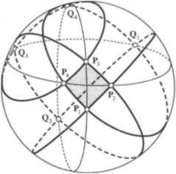
Rational tensor-product surface patches on quadrics have been studied in [10] using the generalized stereographic projection. Here we will only mention a particular result concerning bi-quadratic patches on a sphere; one may consult [10] for a more general discussion. Given four circular arcs forming the closed boundary of a four-sided region on S2, let Pibe the four consecutive corner points of the region, i = 1, 2, 3, 4. See Figure 31.3. Each point Piis an intersection of the two circles that contain the two boundary segments meeting at Pi; let Qidenote the intersection of the two circles that is other than Pi. It is shown in [10] that there exists a bi-quadratic rational Bézier surface on S2 interpolating the given boundary if and only if P1, P3, Q2, and Q4are on the same circle (i.e., these points are coplanar) and the pair P1, P3and the pair Q2, Q4, are not interleaved on that circle.
Further studies on the construction of surface patches on quadrics can be found in the literature [4],[10],[14],[35]. Given three homogeneous variables (r,s,t), the Veronese surface is the 2D surface (r2, s2, t2, rs, st, st) embedded in P5, the five-dimensional projective space [16]. By treating a rational quadratic surface in P3 as a projection of the Veronese surface from P5, Albrecht [1] devises a procedure to determine whether a rational quadratic surface is a quadric surface. Determining if a faithful rational quadratic surface is a quadric can also be carried out by generating the implicit equation of the surface via elimination theory and then examining the degree of the implicit equation.
31.3 FITTING, BLENDING, AND OFFSETTING
In this section we discuss the properties of quadrics concerning the following applications in geometric modeling: fitting, blending, and offsetting. By fitting we mean arranging a collection of surface patches with a certain degree of geometric continuity to pass through an array of data points in 3D space. Blending refers to the smooth joining of quadric surfaces by some other simple surfaces, such as part of a cyclide or a low-degree algebraic surface. The low algebraic degree of quadrics makes them valuable for modeling the boundary of 3D objects because it is then relatively easy to check whether a given point lies inside such an object or to perform fast ray-tracing rendering of quadrics. We will also examine some results about the self-intersection and rationality of offset surfaces to quadrics.
31.3.1 Fitting
The application of quadric surfaces to data fitting originated in the use of quadratic functions to fit data points sampled from a bivariate function [33]. Suppose that a bivariate function f(x,y) is sampled at a collection of points (xi, yi), and the function values and gradients (f(xi,yi), ∇f(xi,yi)) are extracted and associated with (xi, yi). Suppose also that there is a triangulation of the data points (xi, yi). Powell and Sabin [33] study the problem of using quadratic functions to interpolate the data points over each triangle to give a smooth approximation of f(x,y) across the entire domain. Since the graph of a quadratic function is either a paraboloid or a parabolic cylinder, this problem is a specialcase of surface modeling with quadric patches.
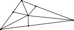
Each quadratic function has six free parameters, but the data points at the vertices of a triangle impose nine constraints; therefore it is, in general, impossible to use a single quadratic function to interpolate over a triangle. A method is presented in [33] that uses a C1 piecewise quadratic function over each triangle which is subdivided into six smaller triangles by connecting each vertex and a point on each side of the triangle to an interior point (see Figure 31.4). Six quadratic functions over the six sub-triangles can be constructed to form a piecewise C1 function over the triangle and this produces a global C1 approximation of the function f(x,y) over a triangulation of the data points (xi, yi).
Subsequent schemes using triangular quadric patches for scattered data interpolation in 3D space adopt a similar approach using more than one triangular quadric patch to cover each triangle domain, to overcome the insufficient degrees of freedom of a single quadric surface. A collection of triangular quadric patches joined with G1 continuity over a properly subdivided triangular domain is called a macro patch. The problem of using triangular quadric patches to fit 3D data, while also matching specified normal vectors at the data points, was first solved by Dahmen [8], and later independently, by Guo [15], both using an algebraic approach. Their conclusion is that, given a triangle with positions and normal vectors specified at the three vertices, one can construct a macro patch consisting of six quadric triangles to interpolate the given data. However, when this scheme is used over a triangulated polyhedral surface formed by scattered data points in 3D space, additional quadric triangles are needed to join macro-patches over adjacent triangles with G1 continuity. A geometric description of this scheme has recently been provided by Bangert and Prautzsch [3].
31.3.2 Blending
The problem of blending quadric surfaces is that of finding a surface, called a blend, which joins different quadric surfaces, called primary surfaces, with a certain degree of continuity. Let an algebraic surface be the zero-set, denoted S(f), of a polynomial f(x,y,z). Let S(f, h) denote the intersection curve between a primary surface S(f) and a clipping surface S(h).
Given two quadric primary surfaces S(f1) and S(f2), and two clipping surfaces S(h1) and S(h2), two curves S(f1,h1) and S(f2, h2) can be defined on S(f1) and S(f2), respectively. The problem of blending S(f1) and S(f2) then becomes that of finding a surface S(g) which is tangential to or has higher-order contact with S(f1) and S((f2) along thecurves S(f1, h1) and S(f2,h2), respectively.
Hoffmann and Hopcroft [17] present a method for surface blending using potential functions. Given two primary surfaces S(f1) and S(f2), consider two families of surfaces S(f1- s) and S(f2- t), with parameters s ∈ [0, ![]() ] and t ∈ [0,
] and t ∈ [0, ![]() ]. Let h1 = f2-
]. Let h1 = f2- ![]() and h2 = f1-
and h2 = f1- ![]() . Then a blend surface of S(f1) and S(f2) can be defined by the algebraic surface swept out by the space curve S(f1- s, f2- t), where s and t satisfy some equation F(s, t)=0, and the curve F(s, t) = 0 is tangential to the s-axis at (
. Then a blend surface of S(f1) and S(f2) can be defined by the algebraic surface swept out by the space curve S(f1- s, f2- t), where s and t satisfy some equation F(s, t)=0, and the curve F(s, t) = 0 is tangential to the s-axis at (![]() , 0) and the t-axis at (0,
, 0) and the t-axis at (0, ![]() ) in the s-t domain to ensure tangency between the blend surface and the primary surfaces. It is recommended [17] that F(s,t) = 0 should be a conic, such as an ellipse, to yield a low-degree blend surface. In this case the blend surface has degree four if S(f1) and S(f2) are quadrics.
) in the s-t domain to ensure tangency between the blend surface and the primary surfaces. It is recommended [17] that F(s,t) = 0 should be a conic, such as an ellipse, to yield a low-degree blend surface. In this case the blend surface has degree four if S(f1) and S(f2) are quadrics.
Warren [46] studies the blending of general algebraic surfaces using the ideal theory of polynomials, and shows that the surface S(g) that is tangential to S(f) along the curve S(f,h) has a special form, i.e., g ∈ I(f,h2), the ideal generated by f and h2. Using this result, Warren obtains quartic blending surfaces for two quadrics, and surfaces of degree six for three-way blending of three quadrics.
Wu and Zhou [48] report a method that produces a degree n + 1 surface for n-way blending of n quadrics, under the condition that the n clipping surfaces are planes that intersect the n primary surfaces in n conics that are contained in a common quadric. C. Chen, F. Chen, and Y. Feng [6] propose a method that uses low degree piecewise algebraic surfaces to blend multiple quadrics. See Figure 31.5for three cylinders joined by a G2 blend that is a piecewise quartic surface produced by their method.
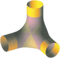
Figure 31.5 A G2 blend for three cylinders by a piecewise quartic surface (Image courtesy of Falai Chen).
There are also other approaches to blending quadrics. Shene [40] uses cyclidal surfaces to blend cones. Wallner and Pottmann [42] use rational surfaces to blend general quadrics.
31.3.3 Offsetting
An offset surface, or offset in short, of a given surface S is the set of points that have a constant distance d to surface S; surface S is also called the progenitor surface. For a point qon the offset surface, the corresponding point pon the progenitor surface that gives rise to qis called the foot point of q. The offset surface is used in NC machining where a given surface S is milled by a spherical-end cutter of radius d with its center following a path on the offset surface of distance d to surface S. Other applications of offsetting are discussed in [34].
The offset surfaces of general surfaces have been extensively studied; see [31], for example. Here we will only discuss some results concerning the offsets of quadric surfaces in the following two aspects: 1) the self-intersection of an offset surface to a quadric; and 2) the rational parameterization of an offset surface to a quadric.
The following discussions concerning offsets will take place in E3, the three-dimensional Euclidean space. We assume that a progenitor surface under consideration is regular and at least twice differentiable; these assumptions are clearly satisfied by nondegenerate quadrics, cylinders, and cones, except at the apex of a cone. By convention, one side of a surface S is assumed to be outside and the other side to be inside, and we assume that the normal vector nat a point pof S always points outside. An offset surface of distance d to progenitor surface S lies outside of S if d > 0, and inside if d < 0. A principal curvature at point pof surface S is assumed to be positive if its center of curvature lies on the opposite side of surface S as pointed to by normal vector n; otherwise, the principal curvature is negative. Let kminand kmaxbe the minimum and maximum principal curvatures, respectively, at point pof surface S. When d > 0 and kmin< 0, the offset surface of distance d has self-intersection due to the local concavity of the surface if d > − 1/kmin; when d < 0 and kmax> 0, the offset surface of distance d has self-intersection if d < − 1/kmax. We will not discuss here the self-intersection of an offset surface due to the global geometry of the progenitor surface, but refer the reader to the more general treatment in [2].
The computation of offset surfaces of natural quadrics, including spheres, circular cones and cylinders, is given in detail by Farouki [12]. The self-intersection problem of an offset surface to a general quadric is studied by Maekawa in two companion papers [25],[26]. The first paper [25] considers the offsets to special quadrics that can be represented by the graph of a quadratic bi-variate function z = f(x,y); these quadrics are the elliptic paraboloid, parabolic cylinder, and hyperbolic paraboloid, which are all the irreducible quadrics tangential to the plane at infinity. It is shown that the self-intersection curve of an offset to such a special quadric is always a segment of a parabola, and this curve degenerates to a straight line in the case of the self-intersecting offset of a parabolic cylinder. When self-intersection occurs, let us call by foot-point curve the curve consisting of the foot points corresponding to the points of the self-intersecting curve on the offset surface; then, in this case, the foot-point curve is the intersection between the progenitor surface and an elliptic cylinder when the progenitor surface is a paraboloid, and the projection of the foot-point curve on the z = 0 plane is an ellipse. The foot-point curve consists of two lines for a self-intersecting offset surface to a parabolic cylinder. Since a surface S can be approximated to the third order by a quadratic paraboloid or a parabolic cylinder in a neighborhood of a regular point of S, the above results, together with asurface curvature analysis, lead to an effective method for detecting the self-intersection, especially small loops, of an offset surface to a general surface, as well as a means to compute an accurate initial point on a self-intersection curve [25].
In the second paper [26] Maekawa studies the self-intersection problem of the offset to a general quadric surface and obtains the following results. The intersection curve of a self-intersecting offset surface to a quadric is, in general, a conic; for example, it is an ellipse for an ellipsoid, an ellipse or hyperbola for a hyperboloid or a cone, depending on the sign of offset distance d, and comprises straight lines for a cylinder. Furthermore, when the progenitor surface S is a non-degenerate quadric or a cone, the foot-point curve corresponding to the self-intersection curve on the offset is the intersection curve of S with an ellipsoid concentric with S; when the progenitor surface S is a cylinder, the foot-point curve corresponding to the self-intersection curve comprises two straight lines that are the intersection between S and an elliptic cylinder. These results are highly useful in understanding and computing the self-intersection of an offset surface to a general quadric.
Next we consider the problem of representing the offset surface to a quadric as a rational surface. Although it is known that any offset surface to a quadric is an algebraic surface, the problem of determining whether such an offset surface is a rational surface has been studied only recently. L ü shows [22] that the offsets to paraboloids and one-sheet hyperboloids are rational, by exploiting the fact that a cubic algebraic surface, except for a cubic cone or cubic cylinder, is a rational surface. Using the same idea, L ü further shows [24] that the offsets to ellipsoids and two-sheet hyperboloids are also rational. It is proven by Pottmann, L ü, and Ravani [32] that the offset to a rational non-developable ruled surface is rational; hence, it also follows from this result that the offsets to a hyperbolic paraboloid and one-sheet hyperboloid are rational.
Although, according to the above results, the offset surface to a non-degenerate quadric is rational, the offset to a properly degenerate quadric, i.e., a cylinder or a cone, is, in general, not rational; the exceptions are parabolic cylinders, circular cones, and circular cylinders, since offset surfaces to these quadrics are easily seen to be rational. These results follow from that the planar offset curve to a hyperbola or an ellipse, except for a circle, is not rational, and that the planar offset curve to a parabola is rational [22],[23].
31.4 INTERSECTION AND INTERFERENCE
31.4.1 Computation of intersection curves
Computing the intersection of two quadrics requires deriving an expression for their intersection curve and determining the topological structure of it. Algorithms for intersecting quadric surfaces can be classified into those taking a geometric approach and those taking an algebraic approach. The geometric approach is numerically more stable but is generally limited to natural quadrics [27],[28],[39]. Below we will confine ourselves to reviewing some algebraic methods developed for general quadrics.
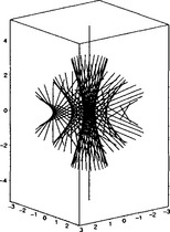
We will refer to the intersection curve of two quadric surfaces as a QSIC. A QSIC is a space curve of degree four. When it is nonsingular, a QSIC can have zero, one, or two disjoint connected components in 3D real projective space, and such a curve does not have a rational parameterization. A nonsingular QSIC is always irreducible. A singularQSIC can be reducible or irreducible. A singular but irreducible QSIC has exactly one singular point, which is a cusp, an acnode, or a crunode, and such a QSIC is a rational quartic curve. A reducible QSIC consists of two or more curves of lower degrees that sum to four; for example, in Figure 31.6two cones intersect in a space cubic curve and a line.
Using the Segre characteristic, Bromwich gives a complete classification of degenerate QSICs in complex projective space, in terms of singularity and reducibility [5],[41]; for two quadrics S0: XT AX = 0 and S1: XT BX = 0, the Segre characteristic is defined by the invariant factors of the quadratic form XT(λA + μB)X. However, these results need to be interpreted in real projective space in order to be useful to CAGD application.
Levin [19],[20] proposes the following algebraic method for computing a QSIC. Let S0: XT AX = 0 and S1: XT BX = 0 be two distinct quadrics. Levin observes that there always exists a ruled quadric in the pencil XT(λA + μB)X = 0; S0and S1are first transformed to simpler forms simultaneously by an affine transformation to facilitate selecting the rule quadric. This ruled quadric, called a parameterization surface, is parameterized by
where R(u) is the base curve of the ruling and T(u) is the direction vector of the generating line passing through R(u). Substituting S(u, v) into either S0or S1, one can solve for v in terms of u to obtain a parameterization of the QSIC of S0and S1of the form
where d(u) is a quartic polynomial, and ![]() (u) and
(u) and ![]() (u) are some vector functions. Only those values of u for which d(u) ≥ 0 give rise to real points on the QSIC.
(u) are some vector functions. Only those values of u for which d(u) ≥ 0 give rise to real points on the QSIC.
Levin’s method is useful for tracing and rendering a QSIC, but does not provide information about the singularity and the structure of the QSIC. In some cases the parameterization computed with Levin’s method may not be appropriate; for instance, whena QSIC is singular or reducible, the method still generates a parameterization involving a square root, although the QSIC has a rational parameterization in this case. Levin’s method was later refined and implemented by Sarraga [36] and also revised and extended by Wilf and Manor [47].
Similar to Bromwich’s work [5], but by studying the eigenvalues and the generalized eigenspaces of the system AB -λI, Ocken, Schwartz, and Sharir show [30] that two quadrics XT AX = 0 and XT BX = 0 can be converted simultaneously by a projective transformation into two canonical forms whose intersection curve can be determined rather easily. The merit of this approach is that a projective transformation is used to convert the pair of input quadrics into forms that are simpler than what are obtained by Levin’s method using an affine transformation. However, the link between the algebraic structure of the eigenspaces and the type of singularity or reducibility of the intersection curve is not discussed fully in [30]. Furthermore, the procedures presented there for classifying and computing the intersection curve are not thoroughly analyzed; for instance, the case of two quadrics intersecting in a line and a space cubic curve is not accounted for, and an intersecting curve having two singular points is listed in one of the generic cases and parameterized using a square-root function, although such a curve is reducible and thus comprises a collection of rational curves. These defects come as no surprise since the authors of [30] seem to be unaware of the classical results by Bromwich based on the Segre characteristic and their results on quadrics in 3D real projective space do not reach the same level of depth as attained by Bromwich [5]. However, it is envisioned that, with a thorough analysis and combining Bromwich’s results, the ideas of Ocken, Schwartz, and Sharir can be further pursued to yield a reliable and complete algorithm for computing QSICs for practical applications.
Farouki, Neff and O′Connor [13] present an alternative algebraic method that uses rational arithmetic to analyze degenerate QSICs. The degeneracy of a QSIC is detected by testing whether the discriminant of the characteristic equation det(λA + μB) = 0 is zero; the discriminant in this case is the resultant of f(λ) ≡ det(λA + μB) and its derivative f′(λ). When the QSIC is found to be degenerate, a quartic projection cone is derived. The reducibility of the QSIC is then determined by factorizing the quartic projection cone.
Wilf and Manor [47] extend Levin’s method to classify a general QSIC as well as to find its expression. To classify a QSIC, the roots of the characteristic equation are obtained numerically, and then the Segre characteristic is computed to guide the parameterization of the QSIC, utilizing Levin’s method. However, this method cannot compute the number of disjoint connected components of a nonsingular QSIC in real projective space, since this information is not provided by the Segre characteristic.
By exploring a birational mapping between a QSIC and a planar cubic curve under stereographic projection with an appropriately chosen center of projection, Wang, Joe, and Goldman [44] develop a method for classifying and computing the QSIC of two general quadrics, through a topological analysis and parameterization of the planar cubic curve. This method produces complete structural information of a QSIC, including the reducibility, the type of singularity, and the number of disjoint connected components of a QSIC in 3D real projective space.
31.4.2 Detecting interference
Interference analysis is about detecting whether two quadrics interfere or intersect with each other. Such problems can be solved by resorting to a general method for computing the intersection curve of two quadrics; however, in interference analysis one is primarily interested in detecting the existence of real intersection points, and thus an expression for the intersection curve is not required. Therefore more efficient methods can be devised for interference analysis.
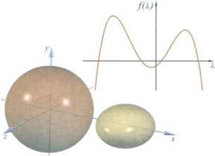
In light of this, an algebraic condition for the separation of two ellipsoids is proved in [45]. Given two ellipsoids XT AX = 0 and XT BX = 0, with A and B normalized so that their first 3×3 minors are positive, it is shown [45] that the characteristic equation det(λA + B) = 0 has at least two real negative roots, and that the ellipsoids are separated by a plane if and only if their characteristic equation has two distinct real positive roots (see Figure 31.7). Furthermore, the ellipsoids touch each other externally if and only if the characteristic equation has a real positive double root. One advantage of this characterization is that only the signs of the roots matter, rather than their exact values.
This approach to interference analysis is related to the Segre characteristic for classifying a degenerate intersection of two quadrics in complex projective space. More research is expected to obtain conditions for discriminating other configurations of two ellipsoids, such as intersection and containment, as well as to perform interference analysis for other quadric surfaces.
31.5 ACKNOWLEDGMENTS
I would like to thank Barry Joe, Ron Goldman, Bert Jüttler, and Myung-Soo Kim for their helpful comments and assistances in writing this chapter. This work has been supported in part by a grant from the Research Grant Council of HKSAR.
1. Albrecht, G. Determination and classification of triangular quadric patches. Computer Aided Geometric Design. 1998;15:675–697.
2. Aomura, S., Uehara, T. Self-intersection of an offset surface. Computer-Aided Design. 1990;22(7):417–422.
3. Bangert, C., Prautzsch, H. Quadric splines. Computer Aided Geometric Design. 1999;16:497–515.
4. Boehm, W., Hansford, D., Béezier patches on quadrics. Farin, ed., eds. NURBS Curve and Surface Design. 1991:1–14.
5. No. 3 Bromwich, T.J., Quadratic forms and their classification by means of invariant-factors. Cambridge Tracts in Mathematics and Mathematical Physics. 1906.
6. C. Chen, F. Chen and Y. Feng. Blending quadric surfaces with piecewise algebraic surfaces. To appear in Graphical Models.
7. Chionh, E.W., Goldman, R.N. Degree, multiplicity, and inversion formulas for rational surfaces using μ-resultants. Computer Aided Geometric Design. 1992;9:93–108.
8. Dahmen, W. Smooth piecewise quadric surfaces. In: Lyche T., Schumaker L., eds. Mathematical Methods in Computer Aided Geometric Design. Academic Press; 1989:181–194.
9. Dietz, R., Hoschek, J., Jüttler, B. An algebraic approach to curves and surfaces on the sphere and on other quadrics. Computer Aided Geometric Design. 1993;10:211–229.
10. Dietz, R., Hoschek, J., Jüttler, B. Rational patches on quadric surfaces. Computer-Aided Design. 1995;27:27–40.
11. Farin, G. NURBS: From Protective Geometry to Practical Use. A.K. Peters; 1999.
12. Farouki, R.T. Exact offsets procedures for simple solids. Computer Aided Geometric Design. 1985;2:257–279.
13. Farouki, R.T., Neff, C.A., O’connor, M.A. Automatic parsing of degenerate quadric-surface intersections. ACM Transactions on Graphics. 1989;8(3):174–203.
14. Geise, G., Langbecker, U. Finite quadric segments with four conic boundary curves. Computer Aided Geometric Design. 1990;7:141–150.
15. Guo, B. Quadric and cubic bitetrahedral patches. The Visual Computer. 1991;11:253–262.
16. Harris, J. Algebraic Geometry – A First Course. Natick, Massachusetts: Springer-Verlag; 1992.
17. Hoffmann, C., Hopcroft, J. Quadratic blending surfaces. Computer-Aided Design. 1986;18(6):301–306.
18. Joe, B., Wang, W. Reparameterization of rational triangular Bezier surfaces. Computer Aided Geometric Design. 1994;11:345–361.
19. Oct Levin, J.Z. A parametric algorithm for drawing pictures of solid objects composed of quadrics. Communications of the ACM. 1976;19(10):555–563.
20. Levin, J.Z. Mathematical models for determining the intersections of quadric surfaces. Comput. Graph. Image Process. 1979;1:73–87.
21. Lodha, S., Warren, J. Béezier representation for quadric surface patches. Computer-Aided Design. 1990;22(9):574–579.
22. Ser. B Lü, W. Rationality of the offsets to algebraic curves and surfaces. Appl. Math. 1994;9:265–278.
23. Lü, W. Offset-rational parametric plane curves. Computer Aided Geometric Design. 1995;12:601–616.
24. Lü, W. Rational parameterization of quadrics and their offsets. Computing. 1996;57:135–146.
25. Maekawa, T. Self-intersection of offsets of quadratic surfaces: Part I, explicit surfaces. Engineering with Computers. 1998;14:1–13.
26. Maekawa, T. Self-intersection of offsets of quadratic surfaces: Part II, implicit surfaces. Engineering with Computers. 1998;14:14–22.
27. October Miller, J.R. Geometric approaches to nonplanar quadric surface intersection curves. ACM Transactions on Graphics. 1987;6:274–307.
28. Miller, J.R., Goldman, R.N. Geometric algorithms for detecting and calculating all conic sections in the intersection of any two natural quadric surfaces. Graphical Models and Image Processing. 1995;57(1):55–66.
29. Minsky, L. An Introduction to Linear Algebra. New York: Oxford University Press; 1962.
30. Ocken, S., Schwartz, J.T., Sharir, M. Precise implementation of CAD primitives using rational parameterizations of standard surfaces. In: Schwartz J.T., Sharir M., Hopcroft J., eds. Planning, Geometry, and Complexity of Robot Motion. Alex Publishing Corporation; 1987:245–266.
31. Pham, B. Offset curves and surfaces: a brief survey. Computer-Aided Design. 1992;24(4):223–229.
32. Pottmann, H., Lü, W., Ravani, B. Rational ruled surfaces and their offsets. Graphical Models and Image Processing. 1996;58(6):544–552.
33. Powell, M.J.D., Sabin, M.A. Piecewise quadratic approximation on triangles. ACM Transactions on Mathematical Software. 1977;3(4):316–325.
34. Rossignac, J.R., Requicha, A.A.G. Offsetting operations in solid modeling. Computer Aided Geometric Design. 1986;3:129–148.
35. Sanchez-Reyes, J., Paluszny, M. Weighted radial displacement: A geometric look at Bézier conies and quadrics. Computer Aided Geometric Design. 2000;17:267–289.
36. Sarraga, R.F. Algebraic methods for intersections of quadric surfaces in GMSOLID. Computer Vision, Graphics and Image Processing. 1983;22(2):222–238.
37. May Sederberg, T.W., Anderson, D.C., Steiner surface patches. IEEE Computer Graphics and Applications. 1985:23–36.
38. Semple, J.G., Kneebone, G.T. Algebraic Protective Geometry. New Jersey: Oxford University Press; 1952.
39. Shene, C.K., Johnstone, J.K. On the lower degree intersections of two natural quadrics. A CM Transactions on Graphics. 1994;13(4):400–424.
40. Shene, C.K. Blending two cones with Dupin cyclides. Computer Aided Geometric Design. 1998;15:643–673.
41. Sommerville, D.M.Y. Analytical Geometry of Three Dimensions. Cambridge University Press; 1947.
42. Wallner, J., Pottmann, H. Rational blending surfaces between quadrics. Computer Aided Geometric Design. 1997;14:407–419.
43. Wang, W., Joe, B., Goldman, R.N. Rational quadratic parameterizations of quadrics. International Journal of Computational Geometry and Applications. 1997;7(6):599–619.
44. preprint Wang, W., Joe, B., Goldman, R.N., Computing quadric surface intersection based on an analysis of planar cubic curves, 2001.
45. Wang, W., Wang, J.Y., Kim, M.-S. An algebraic condition on the separation of two ellipsoids. Computer Aided Geometric Design. 2001;18:531–539.
46. Warren, J. Blending algebraic surfaces. ACM Transactions on Graphics. 1989;8(4):263–278.
47. Wilf, I., Manor, Y. Quadric surface intersection: shape and structure. Computer-Aided Design. 1993;25(10):633–643.
48. Wu, T.R., Zhou, Y.S. On blending several quadratic algebraic surfaces. Computer Aided Geometric Design. 2000;17:759–766.