Geometric Fundamentals
The following recalls the facts and terminology mostly used in Geometry. It may serve also as a first introduction to geometric tools, for more detailed and founded descriptions see the list of references, in particular [7]. Without additional effort most of the discussed topics can be presented in spaces of any dimension.
2.1 AFFINE FUNDAMENTALS
Many properties of computational geometry and its applications do not need the distance of points but only the concepts of parallelism and ratio.
2.1.1 Points and vectors
In general a point in n-space is fixed by its coordinates with respect to some Cartesian system1. Nevertheless, we start our observations with affine aspects.
Let a = [α1 … αn]t and b = [β1 … βn]t denote two points, its difference v = b − ais called a vector, and one has b = a + v. In particular the column o = [0 … 0]t = a − adenotes the null-vector.
Let a0, …, addenote d + 1 points in n–space, d ≤ n. The d vectors vi = ai- a0, i = 1, …, d, are called linearly dependent if α1v1 + ˙˙˙ + αdvd = o, with at least one nonzero αi, otherwise these vectors are called linearly independent. If v1,…, vdare linearly independent, then they span a linear space Vd, and the points a0,…, adare called affinely independent and span an affine space Ad, d is called their dimension.
2.1.2 Affine systems
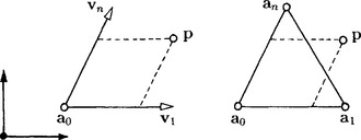
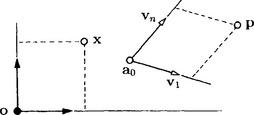
A point a0and n linearly independent vectors videfine an affine system [a0, v1 … vn] of the An. In this system every point p = [η1 … ηn]t can be written uniquely as
where A = [v1 … vn] and x = [ξ1 … ξn]t. The ξiare called the affine coordinates of pwith respect to [a0, v1 … vn], a0is called the origin of the affine system.
To distinguish between points and vectors described by elements aof the ![]() n one may add a further coodinate, ∈, where
n one may add a further coodinate, ∈, where

This convention can help to avoid mistakes in handling with points and vectors, see also Sub section 4.1 on homogeneous coordinates.
2.1.3 Barycentric coordinates
Let a0,…, andenote n + 1 affinely independent points of the An and let vi = ai- a0. One may rewrite equation (1) as
The ξ0, …, ξnare called barycentric coordinates of pwith respect to the frame [a0 … an].
Note that ξ0+˙˙˙+ξn = 1. Note also that any n of the ξi, i ≠ j, represent affine coordinates of pwith respect to an affine system with origin aj.
It follows immediately that a vector v = b−ahas barycentric coordinates v0, …, vnthat sum to zero, v0+…+ vn = 0. Note that the sum of the coordinates ξior vicorresponds to ∈ above.
2.1.4 Affine subspaces and parallelism
Let points a0,…, ad ∈ An be given. The point
is called an affine combination of the points ai. Let d ≤ n and let the points aibe affinely independent. Then they span a d-dimensional subspace ⊂ An. With barycentric coordinates its points are written as affine combinations or with affine coordinates as
where vi = ai- a0. This subspace is called a line, plane or hyperplane if d = 1, 2 or n − 1, respectively.
For any given pand given a0, v1, …, vdas elements of Rn, the linear combination (2) represents a system of n linear equations for the ξi. It is solvable only if plies in the subspace.
Conversely, for varying ξithe presentation (2) can be viewed as the solution of some linear system of n- d equations for an unknown p = [η1 … ηn]t. In particular, if d = n − 1, this system consists of one linear equation, say
or with barycentric coordinates of p
where additionally η0 + … + ηn = 1.
Hyperplanes are called linearly independent if the rows [u0u1 … un] of their coefficients are linearly independent. Consequently, a subspace of dimension d of An can be obtained as the intersection of n- d linearly independent hyperplanes. In particular, a point can be obtained as the intersection of n hyperplanes.
Note that the points of an affine subspace solve an inhomogeneous system, while their differences, the vectors, solve the corresponding homogeneous system.
A line p = a + λvis called parallel to a subspace B ⊂ An if the coordinates of its points solve the homogeneous system corresponding to B. Moreover, two affine subspaces Aand Bare parallel if all lines of Aare parallel to B, or vice versa.
2.1.5 Affine maps and axonometric images
Equation (1) allows two interpretations. First, it expresses pwith respect to a new affine system [a0, v1 … vn], where x = [ξ1 … ξn]t are the new coordinates of p. For example, the equation u0 + utp = 0 of a hyperplane reads in the new coordinates q0 + qtx = 0, where q0 = u0 + uta0and qt = ut A.
Second, it represents an affine map φ: x → p, where xand prepresent affine coordinates of two points. In particular, φ maps the origin o = [0 … 0] and the unit vectors2ei = [δi,1 … δi,n]t into a0and vi, i = 1,…, n, respectively. This important property defines the map uniquely and allows a simple design and investigation of an affine map. Note that φ maps the points xof the hyperplane q0+ qtx = 0 above into the points pof the hyperplane u0+ utp = 0.
If the barycentric coordinate columns of points are denoted by the corresponding hollow letters, φ is written as
Note that affine maps preserve affine combinations, i.e. one has
and also preserve parallelism and the ratio of parallel distances, i.e. w = λvis mapped into [φw] = λ[φv].
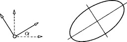
If the viare linearly dependent, the map is degenerated. In particular, if ηd +1 = … = ηn = 0 for all x, the map creates an axonometric image as used in descriptive geometry. Simple examples are the so-called cavalier and military projections, see [7].

2.1.6 Affine combinations and A-frame
Many algorithms in CAGD are based on repeated affine combinations. Consider two points, a0and a1. The affine combination
represents a point on the line spanned by a0and a1, and α represents an affine scale with α = 0 corresponding to a0and α = 1 corresponding to a1.
The term r[p; a0a1] = α/(1 − α) is called the ratio of pwith respect to a0a1.
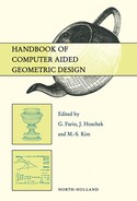
Consider three points a0, a1, a2, and the affine combinations
both related by the same α, and the subsequent affine combination
Obviously, the resulting point pis symmetric in α and β. This means that α and β can be interchanged. This symmetry property is referred to as A-frame lemma and is a fundamental tool in de Casteljau’s work [6].
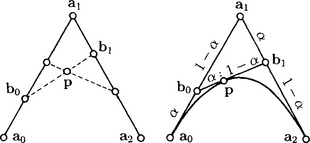
Let α = β. Then (3) reduces to
For fixed α the involved six points represent the so-called affine A-Frame, which is of great importance in Bernstein-Bézier methods. For varying α the point ptraces out a parabola, defined by a0and a2with tangents that intersects in a1.
2.2 CONIC SECTIONS AND QUADRICS
The simplest figures in affine space besides lines and planes are conic sections, or more general, quadrics. They are studied conveniently by their quadratic equations, see [7].
2.2.1 Quadrics in affine space
In an affine space a quadric Qconsists of all points xsatisfying a quadratic equation
where C = Ct is a symmetric non-zero matrix.
The intersection with a subspace is a quadric again. In particular, if the subspace is a line, one gets a pair of points. Note that these points can be real, coalescing or non-real.
A point mis called a midpoint of Q, if Q(x, x) is symmetric with respect to m. This is the case for all solutions of
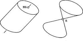
Note that a solution may not exist. If a midpoint slies on Q, it satisfies
and is called a singular point, while Qdegenerates to a cone.
2.2.2 Tangents and polar planes
A line L, given by x = q+ λv, where qis a point of Q, intersects Qin a second point. If both points coalesce, then Lis a tangent of Qat qand satisfies
If additionally vt Cv = 0, then Llies completely on Q, and is called a generatrix of Q. Let v = q−x, then Lis a tangent if
This equation for xrepresents a plane, the tangent plane of Qat q.

Replacing qby an arbitrary point pgives
It represents the polar plane Pof the pole pwith respect to Q. It intersects Qin points qwith tangent planes through p. Note that these points qneed not be real. Note also that Q(p, x) is symmetric in pand x.
A pair of points p, xis called conjugate with respect to Qif Q(p, x) = 0. Hence the points of Qare self-conjugate with respect to Q. A pair of directions u, vis called conjugate with respect to Qif ut Cv = 0. Conjugate elements play an important role in further investigations on quadrics in affine space.
Quadrics differ by the dimension of their midpoints or singularities, the dimension of their real generatrices and in affine space by the shape of their extensions to infinity.
2.2.3 Pascal’s and Brianchon’s theorems
From the past there is a lot of knowledge on conic sections. Of particular interest are the following two theorems on conic sectioncs in the plane:
The three pairs of opposite sides of a hexagon inscribed to a conic section meet in three points of a line (Pascal’s theorem).
The three connections of opposite points of a hexilateral circumscribed to a conic section intersects in one point (Brianchon’s theorem).

As a consequence of these theorems a conic section is uniquely determined by five points or five tangents in the plane.
Of particular interest are the theorems if pairs of consecutive points or tangents coalesce. E.g., let a0, a2denote two points of a conic section with tangents meeting at a point a1. Let the points
span a third tangent. Its point of contact pis easily obtained from Brianchon’ theorem,
where α and β as in (4), see also [6].

2.3 THE EUCLIDEAN SPACE
The affine space An is a Euclidean space denoted by En and the corresponding vector space Vn a Euclidean vector space if a dot product a˙ b = atbis given.
2.3.1 Cartesian coordinates
An affine system [a0, v1… vn] of En is called Cartesian if3vi⋅ vj = δi,jand it is positively oriented if det[v1… vn] >0.
In Cartesian coordinates the distance of two points pand qis given by the length ||v|| of the vector v = q−p,
and the angle ϕ of two vectors uand vis given by
In particular, both vectors are called orthogonal if cos ϕ = 0, i.e. if utv = 0.
2.3.2 Gram-Schmidt orthogonalization
A Cartesian system [a0, b1… bd] of a subspace or the Euclidean space itself can easily be constructed from an affine system [a0, v1… vd] in En with Gram-Schmidt’s orthogonalization by alternating computation of the coefficients λi,jand μias follows:
Set b1 = μ1v1such that ||b1|| = 1.
Set b2 = μ2(v2+ λ2,1b1) such that b2is orthogonal to b1and ||b2|| = 1.
Set ![]() ,such that bdis orthogonal to b1, …, bd −1and ||bd|| = 1.
,such that bdis orthogonal to b1, …, bd −1and ||bd|| = 1.
Note that in a Cartesian system the dot product is written as u⋅ v = utv.
2.3.3 Euclidean motions and orthogonal projections
If the frame [a0, v1… vn] is Cartesian, then (1) represents a Cartesian coordinate transformation or a Euclidean motion. Simple examples of motions in 3-space are the translation by vand the rotation around the 3-axis by an angle ζ, in matrices written as

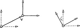
respectively. In particular, let p = Bi(ϕ) xdescribe the rotation around the i-axis by some angle ϕ. Any motion in 3-space can be written as
where α, β, γ are the so–called Eulerian angles.
Any Euclidean motion followed by a map setting the coordinates ηd +1, …, ηnof the image pto zero results in an orthogonal projection onto some d–dimensional subspace.
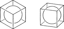
It should be mentioned that orthogonal projections are more informative than simple parallel projections and much more informative then perspectivities. They are the only projections that map spheres to circles. Therefore orthogonal projections should be prefered in presenting technical objects.
2.3.4 Quadrics in Euclidean space
If the vectors viof the Cartesian system [a0, v1… vn] are pairwise conjugate with respect to a quadric Q, then the viare principal axis directions of Qand C is a diagonal matrix.
One easily checks that for a conic section given by its equation a rotation by an angle α where
turns the coordinate axes into the axis directions of Qand transforms C into diagonal form.
2.4 PROJECTIVE FUNDAMENTALS
Introducing points at infinity leads to the projective space and allows a unified and most elegant treatment of geometry4.
2.4.1 Homogeneous coordinates
Let ξ1, …, ξnbe affine coordinates of a point in An with respect to an affine frame [a0, v1…vn] as above. Set ξi = βi/β0with some β0≠ 0. Then the β0,β1, …, βnare homogeneous coordinates with respect to the given affine frame. Note that any non-zero multiple of the homogeneous coordinate column b = [β0β1… βn]t represents the same point. Note also that a point p = o is undefined. It represents the so-called forbidden point.
As before βi = 0, i ≠ 0 represents the coordinate hyperplane ξi = 0. Further, β0 = 0 represents points at infinity lying in the infinite or ideal hyperplane β0 = 0. An affine space An together with its ideal hyperplane forms a projective space Pn, the projective extension of An.
The advantage of this extension is the symmetry of homogeneous coordinates. Points at infinity are handled as points in any other plane. In particular, ideal points allow to intersect parallel lines and subspaces - at infinity. Note that any non-zero multiple of a vector represents the same point at infinity.
Note also that β0 = 0 and β0≠ 0 correspond to ∈ = 0 and ∈ = 1 in 1.2above.
2.4.2 Projective coordinates
Let O0,…, Odbe linearly independent columns of homogeneous coordinates of d +1 points in Pn with integrated factors such that the sum O = O0+⋅⋅⋅+ Odrepresents a given further point O called the unit point. These d +2 points determine a projective frame [O0, …, Od; O] of some projective subspace Sspanned by the points O0,…, Od. Any point p of this subspace can be represented by homogeneous projective coordinates x = [ξ0… ξd]t as

In particular, if oi = [1, ati]t, and o = [1, at]t then ais the center [a0+ … + ad]/d of the aiand the ξiare a multiple of the barycentric coordinates of pwith respect to the affine frame [a0… ad].
2.4.3 Projective maps
The representation (5), with matrices written as ρp = Ax, allows two interpretations. First it represents the point p ∈ Sby new homogeneous coordinates p ∈S. Second it represents a projective map ψ: x → p of Sinto Pn.
In particular, ψ maps the fundamental points xi = [δ0,i… δd,i]t into oi, i = 0, …, d and the unit point [1 … 1]t into o. This determines the projective map uniquely - and A except for a common factor ρ.
Note that a projective map does not preserve parallelism and ratio in general, but it preserves the cross ratio
In particular, if ![]() then both pairs of points, xy and ob, lie in harmonic position. For example, let α be an affine scale, see 1.6, the pairs of points corresponding to −1, +1 and 0, ∞lie in harmonic position.
then both pairs of points, xy and ob, lie in harmonic position. For example, let α be an affine scale, see 1.6, the pairs of points corresponding to −1, +1 and 0, ∞lie in harmonic position.
2.4.4 The procedure of inhomogeneizing
Any homogeneous equation in projective coordinates can easily be inhomogeneized by setting the homogeneizing coordinate to one. Any point ![]() is simply inhomogeneized to xor v, respectively.
is simply inhomogeneized to xor v, respectively.
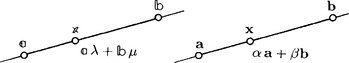
Of particular interest is the application of this procedure to the point x of a projective line given by
Let ρ = 1 and let o = [α0, α0at]t and b = [β0, β0bt]t. Then inhomogeneizing x = [ξ0, ξ0xt]t results in the affine combination
Similar results one gets by inhomogeneizing the points of a projective subspace (5) of higher dimension.
2.4.5 Repeated projective combinations
Repeated affine combinations and A-frames are often used in CAGD to compute polynomial curves and surfaces and can also be applied to the homogeneous coordinates of rational curves and surfaces. It is useful to inhomogeneize the resulting projective combinations by the procedure demonstrated above.
Moreover, after a first inhomogeneizing one can continue with the affine representation of the projective A-frame presented in Subsection 2.3. For more details on this procedure and its applications see [6].
2.4.6 Quadrics in projective space
In homogeneous or projective coordinates o the equation of a quadric Qsimplifies to
and the polarity is written as
Note that in homogeneous coordinates the midpoint of Qis the pole of the infinite plane. Note also that Qis a cylinder, if it has a singular point at infinity, etc.
2.4.7 Parametrizing a quadric and its equation
If a quadric Qis given by its equation ![]() , and q represents a point of
, and q represents a point of ![]() , then
, then
is a parametrization of Q, which is quadratic in the coordinates of p.
Setting, e.g., p = p0ζ0+⋅⋅⋅+pn −1ζn −1, where the piare suitably choosen, it is also quadratic in the homogeneous ζi. Note that one may use any other representation for p, e.g., polar coordinates with the center q.

Conversely, the equation ![]() of a quadric in An or Pn depends on r = (n + 1)(n + 2)/2 homogeneous coefficients, the elements of
of a quadric in An or Pn depends on r = (n + 1)(n + 2)/2 homogeneous coefficients, the elements of ![]() . Let r − 1 pairs of conjugate points, piand qi, be given, and let x denote some arbitrary point of Q. Then the r − 1 conditions
. Let r − 1 pairs of conjugate points, piand qi, be given, and let x denote some arbitrary point of Q. Then the r − 1 conditions ![]() together with
together with ![]() form a homogeneous linear system for the r unknown coefficients of
form a homogeneous linear system for the r unknown coefficients of ![]() . Setting its determinant to zero results in the equation of Q.
. Setting its determinant to zero results in the equation of Q.
2.5 DUALITY
In homogeneous or projective coordinates the equation of a hyperplane simplifies to
The uiare homogeneous coordinates of the hyperplane – as the ξifor x. Homogeneous coordinates can either represent a point or a hyperplane. Consequently any configuration of points and hyperplanes has a dual configuration of hyperplanes and points, where the dual of a point or hyperplane is a hyperplane or point represented by the same coordinates. More general, the hyperplanes meeting some points b1,…,bdare dual to the points of intersection of the hyperplanes b1,…, bd, and vice versa.
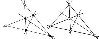
Note that the duality depends on the dimension of the space. For example, Pascal’ and Brianchon’ configuration are dual in the plane, where points and tangents of a conic section are dual elements.
2.6 OSCULATING CURVES AND SURFACES
An important task in CAGD is to connect curves and surfaces smoothly.
2.6.1 Curve and surface
A curve x(t) in affine space An is called regular at t0if ![]() .
.
The curve x(t) is said to have a contact of order r at t0with a surface given by the equation F(x) = 0, if it is regular at t0and if F(x(t)) and its derivatives up to order r vanish at t = t0. This means geometrically that the curve has r + 1 coalescing points in common with the surface at t = t0. Note that this definition does not depend on the parametrization of x(t). Note also that by its geometric meaning the contact of order r is projectively invariant.
2.6.2 Curve and curve
A second curve y(s) given by the intersection of a number of surfaces contacts x(t) at t0with order r if x(t) contacts all these surfaces at least with order r.
If the second curve y(s) is given parametrically, then both curves have contact of order r at t0if there exists a regular reparametrization t = t(s), for x(t) such that the Taylor expansions of x(t(s)) and y(s) agree at t0 = t(s0) up to order r. This condition can be expressed by the chain rule as a system of r + 1 linear equations. Therefore contact of order r is referred to as chain rule continuity.
For example, a curve and its osculating circle at a point t0have contact of order 2.
2.6.3 Surface and surface
Two surfaces have contact of order r at pif all regular curves that lie on one of them and meet phave at least contact of order r with the other surface. This means that after a suitable reparametrization the Taylor expansions of both surfaces at pagree up to order r.
2.6.4 Contur lines, reflection lines and isophotes
There are some important helpful curves to check the smoothness of surfaces visually.

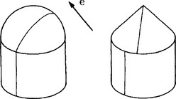
A reflection line on a surface consists of all points pwhose connection with some fixed point e, the eye, is reflected into a ray that meets a given fixed line L.
An isophote on a surface consists of all points pwhose connection with the eye eincludes a fixed angle with the surface normal at p.
Contour lines are special isophotes. They consist of all points p, where the tangent plane meets e.
In general, on composite surfaces contur lines, reflection lines and isophotes have a lower order of contact than the surfaces themselves.
Note that all three kinds of curves can decay in parts. Note also that the use of infinite elements eand Lsimplifies their computation.
2.7 DIFFERENTIAL FUNDAMENTALS
Arc length, curvature and torsion describe the local properties of a curve, the curvature of so-called principal normal sections describe the local properties of surfaces. The main tool for such investigations is a local frame.
2.7.1 Arc length and osculating plane
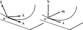
Let a curve in E3 be given parametrically as x = x(t) and let
denote its point and first two derivatives at some t0. If v1≠ 0, its tangent at a0is given by
If ![]() , its osculating plane at a0is given by
, its osculating plane at a0is given by
The differential term ![]() is called the arc element of x(t), and the integral
is called the arc element of x(t), and the integral
its arc length, beginning at t0. The arc length represents the natural parameter of the curve. In most cases it can only be computed approximately.
2.7.2 Curvature and torsion
The natural parameter s is very helpful to derive general curve properties. E.g., let α(s) and β(s) denote the angles of the tangent and the osculating plane at s with the tangent and osculating plane at some s0, respectively, and let the prime ′ denote differentiation with respect to the arc length. Then
are called the curvature and the torsion of x(t) at s0, respectively. Note that ρ = 1/κ represents the radius of the osculating circle.
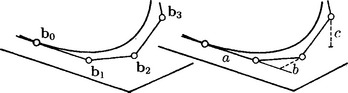
For example, a rational curve of degree n with Bézier points bi = [βi, βibti]t has the span of b0, b1as tangent at b0, and the span of b0, b1, b2as osculating plane at b0. At t = 0 one has
where a, b, c denote the distances of b1from b0, of b2from the tangent at b0, and of b3from the osculating plane at b0, respectively.
2.7.3 The Frenet frame
Schmidt’s orthogonalization applied to ![]() results in the so-called Frenet frame [tmb], which depends on t. One has
results in the so-called Frenet frame [tmb], which depends on t. One has

which is an important tool for further investigations, see [3],[5] and [9].
2.7.4 Curves on surfaces
Let a surface be given parametrically as
The lines u = fixed, v = fixed are called iso-lines. If the partial derivatives xuand xvare linearly independent, the surface normal is defined by
Let u = u(t) denote some curve in the u-plane then, in general, x = x(u(t)) represents a curve on the surface. The arc element ds of this curve is given by its square
where E = xtuxu, F = xtuxv, and G = xtvxvare well–known as Gaussian first fundamental quantities. Note that ||xuΛ xv||2 = EG - F2.

2.7.5 Meusnier’s sphere and Dupin’s indicatrix
Consider all curves on a surface meeting a given point pwith a given tangent tthere. One has:
The osculating circles of these curves lie on a sphere (Meusnier’ sphere).
It follows that the radius of the osculating circle of a surface curve is given by ρ = ρ0cosδ, where δ denotes the angle between the surface normal and the osculating plane and ρ0is the radius of Meusnier’ sphere. The inverse κ0 = 1/ρ0is called the normal curvature of the surface at pin direction of t. Hence it is sufficient to know the curvature of one of these curves and the angle of its osculating plane with nto compute all others.
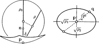
In general, the normal curvature κ0differs for different t. For all tangent directions tat pconsider the points
of the tangent plane with distance ![]() from p. One has: The points qlie on a conic section with center p(Euler’s theorem).
from p. One has: The points qlie on a conic section with center p(Euler’s theorem).
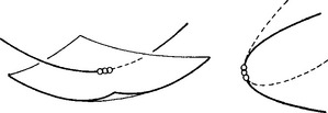
This conic section is also known as Dupin’ indicatrix. Its axis directions are called the principal directions, and the corresponding values of κ = 1/ρ0are called the principal curvatures of the surface at p, mostly denoted by κ1 = 1/ρ1and κ2 = 1/ρ2.
Note that Dupin’ indicatrix can be an ellipse, a pair of parallel lines or a hyperbola. In case of a hyperbola it has two real asymptotic directions. The normal curvature is zero there and ρ0is infinite.
If κ1 = κ2, then Dupin’ indicatrix is a circle and pis called an umbilical or spherical point.
2.7.6 The curvatures of a surface
Because of its geometric meaning Dupin’ indicatrix and consequently the principal curvatures κ1and κ2at a point pdo not depend on the parametric representation of the surface.
are called the Gaussian curvature and the mean curvature of the surface at p, respectively. Both give important information about the smoothness of a surface. Moreover, Gauss has shown that K depends on E, F, and G and their derivatives only. This means that K depends on the inner measurements on the surface only and is invariant under deformations of the surface that do not distort the measurement of lengths on the surface.
1. Adler, C. Modern Geometry. McGraw Hill; 1967.
2. Berger, M. Geometry 1 & 2. New York: Springer; 1987.
3. Boehm, W. Rational geometric splines. Computer Aided Geometric Design. 1987;4:67–77.
4. Boehm, W., Prautzsch, H. Numerical Methods. Berlin: A.K. Peters; 1992.
5. Boehm, W. Differential Geometry I & II, 3rd Edition. Wellesley: Academic Press; 1993.
6. Boehm, W. An affine representation of de Casteljau’s and de Boor’s rational algorithms. Computer Aided Geometric Design. 1993;10:175–180.
7. Boehm, W., Prautzsch, H. Geometric Concepts for Geometric Design. Boston: A.K. Peters; 1994.
8. Boehm, W. Circles of curvature for curves in space. Computer Aided Geometric Design. 1999;16:633–638.
9. do Carmo, M.P. Differential Geometry of Curves and Surfaces. Wellesley: Prentice Hall; 1976.
10. Coxeter, H.S.M. Introduction to Geometry. Englewood NJ: John Wiley & Son; 1969.
11. Farin, G. Curves and Surfaces for CAGD: a Practical Guide, 3rd Edition. New York: Academic Press; 1993.
12. Farin, G., Hansford, D. The Geometry Toolbox for Graphics and Modelling. Boston: AK Peters; 1998.
13. Farin, G. The Essentials of CAGD. Natick MA: AK Peters; 2000.
14. Hilbert, D., Cohn-Vossen, S. Geometry and the Imagination. Natick MA: Chelsea Publishing Co.; 1990.
15. Ding-yuan, L. Computational Geometry - Curve and Surface Modeling. New York: Academic Press Boston; 1992.
16. to appear Prautzsch, H., Boehm, W., Paluszny, M. Bézier and Spline Techniques. Springer; 2002.
17. Wylie, C. Introduction to Protective Geometry. Berlin/New York: McGraw Hill; 1970.
1Matrix notation is preferred. To simplify the notation, a point as well as its coordinate column will be denoted by the same bold letter. Note that this notation depends on the coordinate system.
2δi,jis the so-called Kronnecker-delta, δi,j = 1 if i = j and = 0 else
4“All geometry is projective geometry” [Arthur Cayley 1821-1895]