
Splines over Triangulations
28.1 INTRODUCTION
In the past 35 years, many research papers have been written on bivariate, respectively multivariate splines. This work has been motivated in many cases by the aim to develop powerful tools for fields of application, such as scattered data fitting, the construction and reconstruction of surfaces and the numerical solution of boundary-value problems.
A natural generalization of the classical univariate spline spaces(cf. [16],[87],[112]) which has been widely considered in the literature is defined w.r.t. triangulations (i.e. a finite set of closed triangles in IR2 such that the intersection of any two triangles is empty, a common edge or a common vertex). For given integers r, q, 0 ≤ r <q, the space of bivariate splines of degree q and the smoothness r with respect to Δ is defined by
where
is the space of bivariate polynomials of total degree q. Many research papers on bivariate splines deal with certain subspaces of Srq(Δ), the so-called super splines. Suppose that ρi,i = 1,…, V, are integers satisfying r ≤ ρi<q, i = 1,…, V, and let θ = (ρ1,…, ρv), where V is the number of vertices of Δ. The space of bivariate super splines with respect to Δ is defined by
In contrast to the case of univariate splines, even standard problems such as determining the dimension and the approximation order of bivariate splines and constructing explicit interpolation schemes for these spaces are difficult to solve. In particular, these spacesare very complex when the degree q approaches the smoothness r, which is one of the fundamental phenomena in bivariate spline theory.
The aim of this survey is to summarize results on splines over triangulations. We organize the paper as follows.
In section 28.2, we survey results on Bernstein-B ézier techniques, which are important for CAGD applications. In the context of bivariate splines these techniques provide a useful tool for analysing the structure of these spaces. section 28.3 deals with the dimension of bivariate spline spaces. In contrast to the univariate case, the dimension of these spaces is not known, in general: the most general results are lower and upper bounds. In section 28.4 and 28.5, we discuss interpolation by bivariate spline spaces S, where S can be the space Srq(Δ) as well as a super spline space Sr, θ q>(Δ). A set {z1,…,zd} in Ω, where d = dim S, is called a Lagrange interpolation set for S if for each function f ∈ C(Ω), a unique spline s ∈ S exists such that s(zi) = f(zi), i = 1,…, d. If also partial derivatives of a sufficiently differentiable function f are involved and the total number of Hermite conditions is d, then we speak of a Hermite interpolation set for S. In section 28.4, we discuss classical finite elements and their modern generalizations, the so-called macro element methods, which lead to Hermite interpolation by super splines. Hermite- and Lagrange interpolation methods for bivariate spline spaces Srq(Δ) are summarized in section 28.5. Most of these methods have been developed recently, in particular local Lagrange interpolation methods for C1 spline spaces. A different method for analysing splines over triangulations is based on so-called multivariate B-splines . This approach is described in section 28.6.
28.2 BERNSTEIN-B éZIER TECHNIQUES
In this section, we describe Bernstein-B ézier techniques. These methods are important for applications in CAGD (cf. [13],[55],[66]). In the context of bivariate splines, these techniques appear to play a fundamental role for mainly two reasons. First, since the Bernstein-B ézier representation of the polynomial pieces is used in many research papers to analyse the structure of the spline space. And second, these techniques allow an efficient and stable computation of bivariate splines.
Let T = [t0, t1, t2] be a triangle with vertices t0, t1, t2in IR2. Given a point u∈ IR2 there exist unique scalars λ0(u), λ1(u), λ2(u) such that
The coefficients λ = (λ0, λ1, λ2) are called barycentriccoordinates. Given T, the Bernstein polynomials![]() of degree q w.r.t. T are defined as
of degree q w.r.t. T are defined as
of a polynomial p ∈ Πq, is then called the Bernstein-B ézier representation of p and bα∈ IR are called the Bernstein-B ézier coefficients of p. The value p(u) can be computed recursively by applying the so-called de Casteljau algorithm, which reads as follows:
where ![]() and
and
The Bernstein-B ézier representation of the polynomial pieces of a spline from Srq(Δ) can be used to translate CT smoothness (across common egdes) into useful conditions (cf. [17],[24],[53]). Let T0 = [t0, t1, t2] and T1 = [t1, t2, t3] be triangles with common edge [t1, t2] and s be a function that is given in the piecewise polynomial Bernstein-B ézier representation:
where bi,α∈ IR. Then, s ∈ Srq({T0, T1}) holds if and only if:
These conditions can be checked by running the Casteljau algorithm for the polynomials
at u = t3. If d is a unit vector in direction of the edge D = [t0, t1], then the partial derivative ![]() of the Bernstein polynomials
of the Bernstein polynomials ![]() is given by
is given by
Analogously, if dl are unit vectors in direction of the edge Dl = [t0, tl+1], l = 0, 1, then the following formula holds for u∈ IR2:
Hence, the partial derivative ![]() of a polynomial p in the representation (28.1) fulfills for u ∈ IR2:
of a polynomial p in the representation (28.1) fulfills for u ∈ IR2:
which can also be computed by applying the de Casteljau algorithm. Moreover, evaluating (28.4) at u = t0yields
This formula expresses the connection of partial derivatives at the vertices and the Bernstein-B ézier coefficients and therefore plays an important role for constructing interpolation sets for bivariate splines (cf. [17],[27],[93],[130]). For further results on Bernstein-B ézier techniques and multivariate polynomials, we refer the reader to [12],[17],[18],[24],[37],[53–55].
We finally note that polynomial surfaces were also studied with the help of a classical tool, the polar form[22],[106],[119]. Given a polynomial F ∈ Πq, the corresponding multiaffin polar form is defined as the unique symmetric multiaffine map ![]() satisfying f(u… u) = F(u). Given F ∈ Πq, in its monomial form
satisfying f(u… u) = F(u). Given F ∈ Πq, in its monomial form
where u = (x, y), the corresponding polar form is given as
where ui = (xi, yi), i = 1,…, q. We remark that among other things, polar forms provide an expression for the B ézier points
they provide a closed form solution for the de Casteljau recurrence (28.2)
and they make it easy to phrase the above smoothness conditions (28.3).
28.3 DIMENSION OF SPLINE SPACES
In 1973, the following question was posed [128]: what is the dimension of Srq(Δ)? Clearly, results on the dimension of spline spaces play an important role for the whole theory. But in contrast to the case of univariate splines, investigations on the dimension of bivariate splines yield to complex mathematical problems. In principle, the only exception is the case r = 0, i.e. continuous spline spaces, where the dimension can be easily found (cf. [113]). For r ≥ 1, this problem becomes highly non-trivial, and has not been yet completely solved. In this section, we summarize the results concerning this subject which were given for arbitrary triangulations and for classes of triangulations. For doing this, following [7], we set: VI = number of interior vertices of Δ, VB = number of boundary vertices of Δ, EI = number of interior edges of Δ, N = number of triangles of Δ.
Given an arbitrary triangulation Δ, the most general results concerning the dimension of bivariate splines are lower and upper bounds. In 1979, the following lower bound [113] was given:
Here, the σiare integers depending on q, r, and the number of edges with different slopes attached to the i-th interior vertex of Δ.
Clearly, the dimension of a spline space is determined if an upper bound can be given that coincides with the lower bound (28.5). In order to establish such an upper bound n, it follows from a standard linear algebra argument that it suffices to construct suitable linear functionals λi, i = 1,…,n, with the property: if λi(s) = 0, s ∈ Srq(Δ), i = 1,…,n, then s ≡ 0. Upper bounds [114] of the following type were developed:
where σiare integers depending on q, r, and the ordering of the interior vertices (see also [107]). Bounds of the above type also hold for spline spaces with respect to more general partitions than triangulations, the so-called rectilinear partitions[79],[114], and such bounds were also given for super spline spaces and for spline spaces in more than two variables [2].
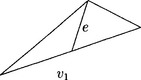
However, it is known that the upper bounds do not coincide with the lower bound (28.5), in general. In fact, there are cases where the dimension of a bivariate spline space is larger than the lower bound (28.5). This was first observed [86] by considering the space S12(Δ MS), where Δ MS is the triangulation as in Figure 28.1. The dimension of this spline space is equal to 7 if Δ MS fulfills certain symmetry properties [127], and otherwise, S12(ΔMS) coincides with Π2. Thus, this example shows that the dimension can depend on geometrical properties of the whole triangulation. In general, such dependencies can appear if the degree q is nearby the smoothness r(see [23],[51]).

We proceed by describing cases where the dimension of Srq(Δ) is known for arbitrary triangulations Δ.
In 1975, the dimension of S1q(Δ), q ≤ 5, was determined [85] by constructing a nodal basis which is based on Hermite interpolation by these spaces. The following formula holds for an arbitrary triangulation Δ:
where σ denotes the number of singular vertices, i.e. interior vertices of Δ that have only two edges with different slopes attached to it. For C1-spline spaces, σi = 1 in (28.5) holds if the corresponding vertex is singular, and in all other cases σi = 0. Therefore, it follows from Euler’s formulas
that (28.6) coincides with the lower bound (28.5). This result was extended [3] to spline spaces Srq(Δ), q ≥ 4r + 1, by coupling the investigations [115] on splines defined on a star (i.e. a set of triangles having one common vertex) with the methods developed in [6],[7]. In these research papers the concept of minimal determining sets was introduced: given a set D of linear functionals defined on S ⊆ S0q(Δ), a set M. ⊆ D is called a minimal determining set for S provided that setting λs for all λ ∈ M uniquely determines s ∈ S. In order to construct such minimal determining sets for spline spaces, the Bernstein-B ézier techniques described in section 28.2 turned out to be useful, since the Bernstein-B ézier coefficients of the polynomial pieces of a bivariate spline can be understood as linear functionals. In this approach one takes advantage of the fact that this type of linear functionals is directly connected to the smoothness conditions of the space via (28.3).
In 1991, the dimension of Srq(Δ), q ≥ 3r + 2, was determined [65] for arbitrary triangulations Δ. This result was generalized [67] to super spline spaces of degree at least 3r + 2 (see also [27]). Again, in these cases the dimension of the (super) spline space coincides with the corresponding lower bound. These results are achieved by using local arguments, i.e. vertices, edges and triangles were considered separately. In particular, it was shown that in these cases a basis of star-supported splines exists. On the other hand, it is known that such a basis does not generally exist if q<3r + 2 and r ≥ 1 (cf. [5]). A result [20] which is connected with this fact was given earlier, where it is shown that in this case the spline spaces are defective in the sense that they do not give optimal approximation order(see section 28.4), in general. Otherwise, i.e. in the case q ≥ 3r + 2, optimal approximation order was shown in several papers by using different methods and by analysing different aspects (cf. [19],[31],[48],[74]).
But the problem of finding an explicit formula for the dimension of Srq(Δ), q<3r + 2, r ≥ 1, w.r.t. arbitrary triangulations Δ remains open. The only exception known from the literature is the space S14(Δ). In 1987, it was shown [7] by using arguments from graph theory which are not purely local that the following formula holds for any Δ:
Again, this number coincides with the lower bound (28.5).
One case of particular interest in spline theory is the case of cubic C1 splines, since it can be seen from the lower bound (28.5) that its dimension must always be larger than the number of vertices of Δ. This is in contrast to the case S12(Δ), where the lower bound (28.5) equals VB + Σ + 3. The literature shows that the structure of the space S13(Δ) is very complex. In fact, at the time of writing of this survey it is still unknown if the dimension of S13(Δ) is always equal to the lower bound 3VB + 2VI + σ + 1, which has been widely conjectured. By using a homological approach [11] it was shown that this conjecture holds generically. In addition, the above conjecture holds for general classes of triangulations. In connection with an interpolation method it was proved [47] that the dimension of S13(Δ) equals the lower bound (28.5), when Δ is contained in the natural class of nested polygon triangulations(see section 28.5). Moreover, a numerical algorithm for determining the dimension of S13(Δ) was discussed in [60].
We proceed by describing results on the dimension of spline spaces w.r.t. general classes of triangulations.
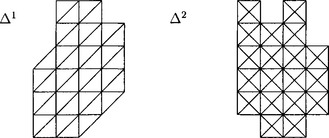
The dimension of Sr3r + 1(Δ), r ≥ 2, was determined [4] for the general class of non-degenerate triangulationsΔ, i.e. triangulations that do not contain degenerate edges(see Figure 28.2).
Moreover, results on the dimension for uniform type triangulations exist in the literature. These are Δ1 and Δ2 triangulations, i.e. triangulations as in Figure 28.3. The dimension of such type of spline spaces, and more generally for so-called crosscut partitions(see Figure 28.4), was determined for arbitrary q and r[28],[29] (see also [114],and for so-called quasi crosscut partitions[80]). For these spline spaces a basis consisting of the polynomials, truncated power functions and so-called cone splines exists. If such triangulations become non-uniform, i.e. the length of the edges of the underlying quadrangulation are allowed to be different, then the dimension is known in the cases r = 1, q ≥ 2, (for Δ1) and r ∈ {1, 2}, q ≥ r + 1, (for Δ2).
In the next two sections, we describe interpolation methods for bivariate (super) splines. We finally remark that the dimension of the spline spaces considered there is always determined.
28.4 FINITE ELEMENT AND MACRO ELEMENT METHODS
In this section, we describe classical finite element methods and its modern extensions, the so-called macro element methods. These are Hermite interpolation methods for bivariate splines, which for low degree splines are based on a suitable splitting procedure applied to every triangle or quadrilateral.
We begin with the classical finite elements (cf. [99]). In 1968, a method [8] was developed which is based on choosing a suitable spline space such that interpolation by bivariate polynomials on every triangle of an arbitrary triangulation Δ automatically leads to Hermite interpolation by C1 splines. In this method, the super spline space S51, θ 1(Δ), where θ1 = (2,…, 2) is used and every polynomial piece in Π5is determined separately by interpolating function value, first and second-order derivatives at the vertices, and the cross boundary derivative at the midpoint of each edge (see Figure 28.5). This approach was generalized [132],[133] to Hermite interpolation by the super spline spaces ![]() where θr = (2r,…, 2r) (see also [81]). A link between this classical method and modern Bernstein-B ézier techniques was given in [116] (for the special case S92, θ 2(Δ), see also [130]).
where θr = (2r,…, 2r) (see also [81]). A link between this classical method and modern Bernstein-B ézier techniques was given in [116] (for the special case S92, θ 2(Δ), see also [130]).
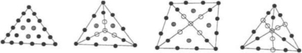
Figure 28.5 The classical finite elements of Argyis, Fried-Scharpf, Clough-Tocher, Fraijs de Veubecke and Sander, and Powell-Sabin (from the left to the right): the Bernstein-B ézier coefficients determined by the interpolation conditions at the vertices are symbolized by black circles, the coefficients determined by the cross boundary derivatives are symbolized by grey circles, and the remaining coefficients determined by the differentiability properties are symbolized by white circles.
In order to keep computational costs small, it is desirable in general, however, to use low degree splines in relation to the smoothness. The following classical methods have been developed for this purpose. The idea of these approaches is to modify the given partition, which can be a triangulation or a convex quadrangulation. In contrast to the finite element method described above, more than one polynomial piece is needed for each triangle or quadrilateral such that the method is local. These classical approaches leadto Hermite interpolation by cubic and quadratic C1 splines.
In 1966, a Hermite interpolation set for S13(ΔCT) was constructed [34] (see also [32],[33], [52]) where ΔCT is a triangulation obtained from an arbitrary triangulation Δ by splitting each triangle T ∈ Δ into three subtriangles, the so-called Clough-Tocher split. This Hermite interpolation set consists of function and gradient value at the vertices of Δ and the cross boundary derivative at the midpoints of all edges of Δ (see Figure 28.5).
Another classical scheme [57],[111] for cubic C1 splines works for triangulated convex quadrangulations (see also [72]). Such triangulations are obtained from a set of convex quadrilaterals by adding both diagonals to every quadrilateral. The corresponding Hermite interpolation set consists of function and gradient value at the vertices and the cross boundary derivative at the midpoints of all edges of the underlying convex quadrangulation (see Figure 28.5).
In 1977, quadratic C1 splines were considered [105] that interpolate function and gradient value at all vertices of an arbitrary triangulation Δ (see Figure 28.5). The splines were defined w.r.t. the so-called Powell-Sabin triangulation Δps, which is obtained by splitting every triangle T ∈ Δ into six subtriangles. Here, the splitting points are chosen such that each interior edge of Δ leads to a singular vertex of ΔPS(see section 28.3). For further results on the Powell-Sabin element and a modification of it, we refer to [40],[63],[110]. A multiresolution analysis based on quadratic Hermite interpolation using Powell-Sabin splits has recently been constructed in [36].
We proceed by describing modern extensions of the above classical methods to spline spaces of higher smoothness, the so-called macro element methods. These methods were developed by using Bernstein-B èzier techniques. In contrast to the above classical elements and the methods described in the next section, these extensions lead to interpolation by super spline subspaces.
We start with the generalizations of the Clough-Tocher element. In 1994, Hermite interpolation sets were constructed [69] for certain super spline spaces ![]() where r is odd and
where r is odd and ![]() where r is even. These sets consist of function value and derivatives up to a certain order at the vertices and suitable derivatives at interior pointsof each edge of the given triangulation Δ. Later, this method was improved [76] by reducing the number of degrees of freedom. The corresponding Hermite interpolation sets for such splines contain, in addition, the function values and derivatives up to a certain order at the splitting points. An example of this construction is given in Figure 28.6.
where r is even. These sets consist of function value and derivatives up to a certain order at the vertices and suitable derivatives at interior pointsof each edge of the given triangulation Δ. Later, this method was improved [76] by reducing the number of degrees of freedom. The corresponding Hermite interpolation sets for such splines contain, in addition, the function values and derivatives up to a certain order at the splitting points. An example of this construction is given in Figure 28.6.
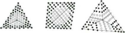
Figure 28.6 The macro elements of Lai-Schumaker (from the left to the right): the Bernstein-B ézier coefficients determined by the interpolation conditions at the vertices are symbolized by black circles, respectively by a grey box, the coefficients that can be determined by cross boundary derivatives across the edges are symbolized by grey circles, and the remaining coefficients determined by the differentiability properties are symbolized by white circles.
A generalization of Fraeijs de Veubecke’s and Sander’s method for splines on triangulated convex quadrangulations was also developed [70]. The following cases were considered: ![]() if r is odd,
if r is odd, ![]() if r is even. Here, the components of θ concerning the vertices of the underlying quadrangulation are 3r- 1/2 if r is odd and 3 r /2 if r is even. The corresponding Hermite interpolation method is to interpolate function value and derivatives up to order r + [r/2] at the vertices and suitable derivatives at interior points of each edge of the underlying quadrangulation. For such type of triangulations Δ a quasi interpolation method for the space
if r is even. Here, the components of θ concerning the vertices of the underlying quadrangulation are 3r- 1/2 if r is odd and 3 r /2 if r is even. The corresponding Hermite interpolation method is to interpolate function value and derivatives up to order r + [r/2] at the vertices and suitable derivatives at interior points of each edge of the underlying quadrangulation. For such type of triangulations Δ a quasi interpolation method for the space ![]() was developed [75]. Earlier, the particular case
was developed [75]. Earlier, the particular case ![]() where ρi∈ {2, 3} was investigated [73]. In this case, the quadrilaterals of the underlying quadrangulation do not need to be convex and the super spline property appears only at certain interior vertices. Recently, macro elements for the above type of spline spaces were constructed [78] with the aim of removing certain degrees of freedom at the intersection points of the diagonals. This is done by assuming an additional supersmoothness at these points. An example of this construction is given in Figure 28.6.
where ρi∈ {2, 3} was investigated [73]. In this case, the quadrilaterals of the underlying quadrangulation do not need to be convex and the super spline property appears only at certain interior vertices. Recently, macro elements for the above type of spline spaces were constructed [78] with the aim of removing certain degrees of freedom at the intersection points of the diagonals. This is done by assuming an additional supersmoothness at these points. An example of this construction is given in Figure 28.6.
Now, we discuss generalizations of the Powell-Sabin element. In 1996, the triangulation Δ1PSwas considered [71]. This triangulation is obtained by applying the Powell-Sabin split to each triangle of a Δ1 triangulation (see section 28.3). There it is shown that the function value and the derivatives up to order r + [r/2] at all vertices of Δ1 build a Hermite interpolation set for the super spline space ![]() if r is odd,
if r is odd, ![]() if r is even, where
if r is even, where ![]() Later, Hermite interpolation sets were constructed [77] for lower degree super spline spaces with respect to Δps. These sets contain, in addition, the function values and derivatives of a certain order at the splitting points. An example of this construction is given in Figure 28.6.
Later, Hermite interpolation sets were constructed [77] for lower degree super spline spaces with respect to Δps. These sets contain, in addition, the function values and derivatives of a certain order at the splitting points. An example of this construction is given in Figure 28.6.
We finally remark that it was shown that the constructions [75–78] yield to so-called stable, local bases, which implies that the associated spline space S has optimal approximation order, i.e., for each sufficiently differentiable f,
where h is the maximal diameter of the triangles and K is a constant depending on no other geometrical properties than the smallest angle in the corresponding triangulation. Such bases have also been constructed for (super) spline spaces of degree q ≥ 3r + 2 on arbitrary triangulations (cf. [31],[45],[74]). In this case, a Hermite interpolation operator of a super spline subspace that yields optimal approximation order, where the corresponding fundamental splines have minimal support was constructed in [48].
28.5 INTERPOLATION BY SPLINE SPACES
Considering the results discussed in the previous sections, the natural problem of constructing interpolation sets for the spline space Srq(Δ) appears. In particular, since the Hermite interpolation methods described above cannot be transformed into Lagrange interpolation on the whole triangulation straightforwardly, the question arises: how canLagrange interpolation sets for spline spaces be constructed? We note that concerning the construction and reconstruction of surfaces, it is sometimes desirable that only function values are involved and no (cross boundary) derivatives have to be estimated. For example, in many practical applications a surface is described by a linear spline on a fine triangulation (i.e. with many triangles), and an interpolating spline on a coarse subtriangulation can then be constructed by taking the Lagrange data directly from the linear spline.
Since interpolation by splines is strongly connected with the problem of determining the dimension, the literature shows that it is a complex problem to construct explicit interpolation schemes for Srq(Δ), and in particular for Lagrange interpolation. Indeed, there are cases where not even one single Lagrange interpolation set is known. However, as described below, many efficient interpolation methods were developed for splines of certain degree q and smoothness r w.r.t. certain classes of triangulations. Moreover, we mention that in contrast to the case of univariate splines, Schoenberg-Whitney type conditions do not characterize interpolation by bivariate splines : the natural multivariate analogue of such conditions [42],[49] characterizes almost interpolation, but not interpolation (see also [124]).
In this section, we summarize results on Hermite- and Lagrange interpolation by spline spaces.
First, it is obvious that a Lagrange interpolation set for ![]() is obtained by the union of all points
is obtained by the union of all points ![]() where T = [t0, t1, t2] is a triangle in Δ with vertices t0, t1, t2. In particular, the set of vertices of Δ is a Lagrange interpolation set for S01(Δ). An algorithm [30] for constructing more general Lagrange interpolation sets for S01(Δ) was given in 1986, and recently, a characterization [50] of Lagrange interpolation sets for S01(Δ) was found. For r ≥ 1 the interpolation problem becomes more complex. In this case, explicit interpolation schemes were given in the literature for certain classes of triangulations respectively for splines of certain degree q and smoothness r. In the following we describe these methods.
where T = [t0, t1, t2] is a triangle in Δ with vertices t0, t1, t2. In particular, the set of vertices of Δ is a Lagrange interpolation set for S01(Δ). An algorithm [30] for constructing more general Lagrange interpolation sets for S01(Δ) was given in 1986, and recently, a characterization [50] of Lagrange interpolation sets for S01(Δ) was found. For r ≥ 1 the interpolation problem becomes more complex. In this case, explicit interpolation schemes were given in the literature for certain classes of triangulations respectively for splines of certain degree q and smoothness r. In the following we describe these methods.
Many research papers (see for instance [10],[25],[68],[109],[123],[126]) that appeared between 1981 and 1994 investigated the problem of constructing interpolation sets for cubic and quadratic C1 splines w.r.t. uniform type triangulations (see Figure 28.3). Then, in the beginning 90ies, a general method [89],[90] for constructing Lagrange and Hermite interpolation sets for Srq(Δi), i = 1, 2, was developed. The basic idea of this method is to construct line segments in Ω and to place points on these lines which satisfy the interlacing condition of Schoenberg-Whitney for certain univariate spline spaces suchthat the principle of degree reduction can be applied. Figure 28.7shows examples of Lagrange interpolation sets constructed by this method. Hermite interpolation sets for Srq(Δi), i = 1, 2, are obtained by using these Lagrange interpolation sets and by “taking limits”, which means, roughly speaking, that the points are shifted to the vertices. An extension of this method to crosscut partitions was given in [1] (see also [98]). Results on the approximation order of this method can be found in [46],[88],[91].
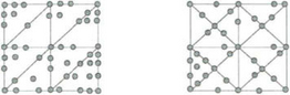
Figure 28.7 Example for the interpolation method of Nürnberger-Rießinger: the Lagrange interpolation points for S14(Δ1) and S13(Δ2) are symbolized by grey circles.
We proceed by describing interpolation methods for classes more general than Δi, i = 1, 2. These classes are triangulations constructed from given points, arbitrary triangulations and general classes of triangulations.
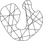
We start with methods [93], where triangulations are constructed which are suitable for Lagrange and Hermite interpolation by Srq(Δ), q ≥ 2r + 1, r = 1, 2. These methods are based on an inductive principle: by starting with one triangle, in each step a set of triangles building a suitable polyhedron is added to the subtriangulation constructed so far. The vertices of these triangles are locally chosen scattered points. The construction of the triangulation is such that the corresponding splines can be extended in each step. Lagrange and Hermite interpolation sets were constructed simultanously, and again, Hermite interpolation sets are obtained by “taking limits”. The corresponding interpolating splines can be computed step by step by using Bernstein-B ézier techniques, where in each step only small linear systems of equations have to be solved. Examples of Lagrange interpolation points inside a polyhedron are given in Figure 28.8. Numerical tests with large numbers of interpolation conditions showed that this interpolation method yields good approximations for S1q(Δ), q ≥ 4, and S2q(Δ), q ≥ 7. In order to obtain good approximations in the remaining cases (for non-uniform triangulations Δ) variants based on applying the Clough-Tocher split (see section 28.4) to some of the triangles were proposed. This general method can be applied to certain classes of given triangulations Δ, in particular the class of triangulated quadrangulations [92]. Moreover, for quadratic C1 splines a general class of triangulations ΔQwas given, where Lagrange interpolation at the (non-singular) vertices together with three additional points in the starting triangle is always possible.
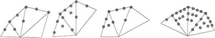
Figure 28.8 Example for the Lagrange interpolation points inside a polyhedron: from the left to the right: ![]()
We now describe interpolation methods for splines on arbitrary and general classes of triangulations.
Hermite interpolation sets for S1q(Δ), q ≥ 5, where Δ is an arbitrary triangulation, were constructed in [43],[85] (see section 28.3). Later, a different method [44] was developed for constructing explicit Hermite and Lagrange interpolation sets in these cases. This approach can also be applied to S14(Δ), where Δ has to be slightly modified if exceptional constellations of triangles occur. Earlier, a Hermite interpolation scheme for S14(Δ) wasdefined [59] in the special case when Δ is an odd degree triangulation, i.e. every interior vertex has odd degree. Moreover, quasi-interpolation by S14(Δ) was considered [26]. There it is shown that optimal approximation order can be achieved by quasi-interpolation, if certain edges are swapped. The case S13(Δ) is more complex since not even the dimension of these spaces is known for arbitrary triangulations Δ (see section 28.3). In 1987, a global approach [60] for constructing Lagrange interpolation sets involving function values at all vertices of a given triangulation Δ was proposed. This method requires to solve a large linear system of equations, where it is not guaranteed that this system is solvable. A method to construct Lagrange and Hermite interpolation for S13(Δ) was given in [47]. In these investigations, Δ is contained in the general class of so-called nested polygon triangulations, i.e. triangulations consisting of nested closed simple polygons whose vertices are connected by line segments. This construction of interpolation sets for S13(Δ) is inductive by passing through the points of the nested polygons in clockwise order: in each step, a point of a nested polygon and all triangles with this vertex having a common edge with the subtriangulation considered so far are added. Then the interpolation points are chosen locally on these triangles, where the number of interpolation points is different if so-called semi-singular vertices exist or not. Numerical examples with a large number of interpolation conditions showed that in order to obtain good approximations, it is desirable to subdivide some of the triangles of Δ. The method of constructing interpolation points also works for these modified triangulations.
Recently, the problem of local Lagrange interpolation for C1 splines was investigated [94],[97]. In this context local means that the fundamental Lagrange splines si determined by Si(zj) = δi,j, j = 1,…, d, have local support. (Here, δi,jdenotes Kronecker’s symbol.) We note that the classical Hermite interpolation methods described in section 28.4 cannot be transformed straigthforwardly into a local Lagrange interpolation scheme on a given triangulation.
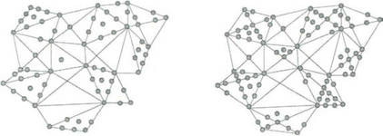
In [94] (see also [95]) an algorithm was developed for constructing local Lagrange interpolation sets for C1 splines of degree ≥ 3. This algorithm mainly consists of two algorithmic steps and is based on an appropriate coloring of the triangles with two colors. Given an arbitrary triangulation Δ, in the first step, Lagrange interpolation points are chosen on the edges of Δ such that the interpolating spline is uniquely determined (only) on the edges. In the second step of this algorithm, the triangles are colored black andwhite (by a fast algorithm) such that at most two neighboring triangles have the same color (see Figure 28.9). Then, the white triangles are subdivided by a Clough-Tocher split, and in the interior of the black triangles, additional Lagrange interpolation points are chosen. Finally, the Lagrange interpolating spline is uniquely determined on the whole triangulation. Figure 28.9 shows an example of such an interpolation set for the case of cubic C1 splines.
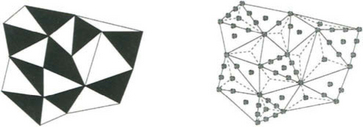
Figure 28.9 Local Lagrange interpolation by cubic C1 splines: the triangles to be splitted result from the coloring of a given triangulation Δ. The Lagrange interpolation points are symbolized by grey circles.
Since recently, the construction of local Lagrange interpolation schemes by cubic C1 splines on quadrangulations of convex quadrilaterals [97] is under investigation. For a special class of triangulated quadrangulations such schemes have been given in [96] (see Figure 28.10). We remark that these interpolation methods yield to optimal approximation order and the corresponding Lagrange interpolating splines can be computed efficiently by using Bernstein-B ézier techniques since the algorithmical complexity of these methods is linear in the number of triangles. Numerical tests given in [94–96] with upto 106 Lagrange interpolation points demonstrate the efficiency of these methods.
28.6 TRIANGULAR B-SPLINES
The results of section 28.4 and 28.5 show that there are many cases where the spline space Srq(Δ) provides powerful tools for applications. On the other hand, the structure of these spaces is very complex, in general. In particular, the discussion of section 28.3 shows that determining the dimension is difficult for arbitrary triangulations. Therefore, it is a complex task to construct suitable basis functions for these spaces, in general.
In this section, we describe a different approach, which was developed with the aim to construct smooth piecewise polynomial basis functions for splines over arbitrary triangulations. This approach is based on a geometrical way to construct smooth piecewise polynomial functions M: IR2 ![]() IR by projecting a polyhedron P ⊂ IRn onto IR2 and by defining M(u) as the (n -2)-dimensional volume of the fibre π−1(u). This definition generalizes the geometric definition of univariate B-splines and hence the resulting functions are called multivariate B-splines. Depending on wether P is just any polyhedron, a box, or a simplex, the resulting multivariate B-splines are also called polyhedral, box, or simplex splines.
IR by projecting a polyhedron P ⊂ IRn onto IR2 and by defining M(u) as the (n -2)-dimensional volume of the fibre π−1(u). This definition generalizes the geometric definition of univariate B-splines and hence the resulting functions are called multivariate B-splines. Depending on wether P is just any polyhedron, a box, or a simplex, the resulting multivariate B-splines are also called polyhedral, box, or simplex splines.
If the given triangulation Δ happens to be of uniform type (see Figure 28.3, for instance), then box splines are the natural choice. Box splines are a natural generalizationof uniform B-splines and have a very rich structure. In particular, they have a stable recurrence and can be generated by subdivision [21]. In the CAGD context, box splines have been first considered in [108], Computational aspects and algorithms for converting to piecewise Bernstein-B ézier representation (28.1) through the use of masks have been given in [14]. Surface fitting with box splines was discussed in [35]. The first book which was completely devoted to box splines is [21].
If an arbitrary triangulation Δ is given, then in this approach simplex splines have to be used. Simplex splines can be defined recursively as follows: Given the knots t0,…, tq + 2∈ IR2 one can show [82],[83] that the recursion
with![]() is well-defined and yields a simplex spline M of degree q that is Cq−1 continuous if the knots are in general position. (Here, d(t0, t1, t2) stands for the area of the triangle T = [t0, t1, t2] multiplied by two.) Further details on simplex splines can be found, e.g., in [15],[38],[61],[84],[122].
is well-defined and yields a simplex spline M of degree q that is Cq−1 continuous if the knots are in general position. (Here, d(t0, t1, t2) stands for the area of the triangle T = [t0, t1, t2] multiplied by two.) Further details on simplex splines can be found, e.g., in [15],[38],[61],[84],[122].
The next problem is to construct a spline space from these functions. While for box splines one can consider the space spanned by translates, this problem is difficult for simplex splines: given an arbitrary triangulation Δ, exactly what simplex splines should be considered?
Solutions to this problem were given first in [39],[64], and later in [41],[121]. These constructions start with a triangulation Δ, where for every vertex tiof Δ a cloud of points ti,0,…,ti,q is assigned. Then a rule of selecting ![]() subsets of q + 3 knots from the three clouds associated with a triangle is given. Each such subset yields a simplex spline of degree q which is generally Cq−1. The linear span Eqof of all these degree q simplex splines is then the spline space of interest. Note that both schemes produce splines over a refined partition of Δ.
subsets of q + 3 knots from the three clouds associated with a triangle is given. Each such subset yields a simplex spline of degree q which is generally Cq−1. The linear span Eqof of all these degree q simplex splines is then the spline space of interest. Note that both schemes produce splines over a refined partition of Δ.
The two schemes differ in the knot selection rule, in the ease of use, and in the class of surfaces that they are able to represent. The first scheme [39],[64] contains the polynomial space, i.e. Πq⊂q, but the representation of arbitrary piecewise polynomials remained unsolved. This defect was overcome by the scheme [41],[121]. The knot selection rule of this scheme is based on the use of polar forms [117],[120] (see section 28.2), and for a given triangle T = [t0, t1, t2] selects the simplex splines
with
Furthermore, the new scheme not only allows the representation of the polynomials, but also allows the representation of piecewise polynomials, i.e. ![]() Moreover, up to normalization, the coefficients in the resulting representation
Moreover, up to normalization, the coefficients in the resulting representation
of a piecewise polynomial F as a linear combination of simplex splines are given as
by evaluating the polar form fT(see section 28.2) of the restriction FT of F to the triangle T = [t0, t1, t2] on a suitable sequence of knots [118]. Note that this formula captures completely the analog formula for the de Boor points in the B-spline expansion of a univariate spline, and also the formula for the Bernstein-B ézier points in the expansion of a polynomial surface in the representation (28.1).
Practical aspects of implementing the simplex spline scheme [41],[121] have been discussed [9],[129]. A first implementation on triangular B-splines has been described in [56],[62]. Efficient evaluation routines for triangular B-splines have been given in [100] for the quadratic case, and in [58] for arbitrary degree q. Here, efficiency is obtained by reusing partial results. Algorithms for surface fitting and modeling with triangular B-splines have been discussed in [102–104]. Finally extensions of the approach to a spherical setting have been presented in [101].
Acknowledgment.
The authors thank Günther Nürnberger for discussing the various topics described in this paper.
1. Adam, M.H. Bivariate Spline-Interpolation auf Crosscut-Partitionen. PhD thesis, University of Mannheim. 1995.
2. Alfeld, P. Upper and lower bounds on the dimension of multivariate spline spaces. SIAM J. Numer. Anal. 1996;33(2):571–588.
3. Alfeld, P., Schumaker, L.L. The dimension of bivariate spline spaces of smoothness r for degree d ≥ 4r + 1. Constr. Approx. 1987;3:189–197.
4. Alfeld, P., Schumaker, L.L. On the dimension of bivariate spline spaces of smoothness r and degree d = 3r + 1. Numer. Math. 1990;57:651–661.
5. Alfeld, P., Schumaker, L.L. Non-existence of star-supported spline bases. SIAM J. Math. Anal. 2000;31:1482–1501.
6. Alfeld, P., Piper, B., Schumaker, L.L. Minimally supported bases for spaces of bivariate piecewise polynomials of smoothness r and degree d ≥ 4r + 1. Computer Aided Geometric Design. 1987;4:105–123.
7. Alfeld, P., Piper, B., Schumaker, L.L. An explicit basis for C1 quartic bivariate splines. SIAM J. Numer. Anal. 1987;24:891–911.
8. Argyis, J.H., Fried, I., Scharpf, D.W. The TUBA family of plate elements for the matrix displacement method. Aeronaut. J. Roy. Aeronaut. Soc. 1968;72:701–709.
9. Auerbach, S., Gmelig Meyling, R.H.J., Neamtu, M., Schaeben, H. Approximation and geometric modeling with simplex B-splines associated with irregular triangles. Computer Aided Geometric Design. 1991;8:67–87.
10. Beatson, R.K., Ziegler, Z. Monotonicity preserving surface interpolation. SIAM J. Numer. Anal. 1985;22(2):401–411.
11. Billera, L.J. Homology of smooth splines: generic triangulations and a conjecture of Strang. Trans. Am. Math. Soc. 1988;310(2):325–340.
12. Boehm, W., Farin, G., Kahmann, J. A survey of curve and surface methods in CAGD. Computer Aided Geometric Design. 1984;1:1–60.
13. Boehm, W., Hoschek, J., Seidel, H.-P. Mathematical aspects of computer aided geometric design. In: Artin M., Kraft H., Remmert R., eds. Duration and Change: Fifty Years at Oberwolfach. Los Alamitos, CA: Springer; 1994:106–138.
14. Boehm, W., Prautzsch, H., Arner, P. On triangular splines. Constr. Approx. 1987;3:157–167.
15. Bojanov, B.D., Hakopian, H.A., Sahakian, A.A. Spline Functions and Multivariate Approximation. Kluwer; 1993.
16. de Boor, C. A Practical Guide to Splines. Dordrecht: Springer; 1978.
17. de Boor, C. B-form basics. In: Farin G., ed. Geometric Modeling. New York: SIAM; 1987:131–148.
18. de Boor, C. Multivariate piecewise polynomials. Ada Numerica. 1993:65–109.
19. de Boor, C., Höllig, K. Approximation power of smooth bivariate pp functions. Math. Z. 1988;197:343–363.
20. de Boor, C., Jia, Q. A sharp upper bound on the approximation order of smooth bivariate pp functions. J. Approx. Theory. 1993;72:24–33.
21. de Boor, C., Höllig, K., Riemenschneider, S. Box Splines. Philadelphia: Springer; 1993.
22. de Casteljau, P. Formes à pôles. Berlin: Hermes; 1985.
23. Chen, Z.B., Feng, Y.Y., Kozak, J. The blossoming approach to the dimension of the bivariate spline space. J. Comp. Math. 2000;18:183–198.
24. CBMS 54 Chui, C.K. Multivariate Splines. Paris: SIAM; 1988.
25. ISNM 81 Chui, C.K., He, T.X. On location of sample points in C1 quadratic bivariate spline interpolation. In: Collatz L., Meinardus G., Nürnberger G., eds. Numerical Methods of Approximation Theory. Philadelphia: Birkhäuser; 1987:30–43.
26. Chui, C.K., Hong, D. Swapping edges of arbitrary triangulations to achieve the optimal order of approximation. SIAM J. Numer. Anal. 1997;34:1472–1482.
27. Chui, C.K., Lai, M.-J. On bivariate super vertex splines. Constr. Approx. 1990;6:399–419.
28. Chui, C.K., Wang, R.H. Multivariate spline spaces. J. Math. Anal Appl. 1983;94:197–221.
29. Chui, C.K., Wang, R.H. On smooth multivariate spline functions. Math. Comput. 1983;41:131–142.
30. Chui, C.K., He, T.X., Wang, R.H. Interpolation by bivariate linear splines. In: Szabados J., Tandori J., eds. Alfred Haar Memorial Conference. Basel: North Holland; 1986:247–255.
31. Chui, C.K., Hong, D., Jia, Q. Stability of optimal-order approximation by bivariate splines over arbitrary triangulations. Trans. Amer. Math. Soc. 1995;347:3301–3318.
32. Ciarlet, P.G. Sur 1’ élément de Clough et Tocher. RAIRO Anal Numer. 1974;2:19–27.
33. Ciarlet, P.G. Interpolation error estimates for the reduced Hsieg-Clough-Tocher triangles. Math. Comp. 1978;32:335–344.
34. Clough, R.W., Tocher, J.L., Finite element stiffness matries for analysis of plates in bending. Proc. Conf. on Matrix Methods in Structural Mechanics. Wright Patterson A.F.B., Ohio, 1965.
35. Dæhlen, M., Lyche, T. Boxsplines and applications. In: Geometric Modelling. Amsterdam: Springer; 1991:35–93.
36. Daehlen, M., Lyche, T., Mørken, K., Schneider, R., Seidel, H.-P. Multiresolution analysis over triangles based on quadratic Hermite interpolation. J. Comp. Appl. Math. 2000;119:97–114.
37. Dahmen, W., Bernstein-Bézier representation of polynomial surfaces. Proc. ACM SIGGRAPH. Dallas. 1986.
38. Dahmen, W., Michelli, C.A. Recent progress in multivariate splines. In: Chui C.K., Schumaker L.L., Ward J.D., eds. Approximation Theory IV. Academic Press; 1983:27–121.
39. Dahmen, W., Micchelli, C.A. On the linear independence of multivariate B-splines, I. Triangulations of simploids. SIAM J. Numer. Anal. 1982;19:993–1012.
40. Dahmen, W., Gmelig Meyling, R.H.J., Ursem, J.H.M. Scattered data interpolation by bivariate C1 -piecewise quadratic functions. Approx. Theory Appl. 1990;6:6–29.
41. Dahmen, W., Micchelli, C.A., Seidel, H.-P. Blossoming begets B-splines built better by B-patches. Math. Comp. 1992;59:97–115.
42. Davydov, O. On almost interpolation. J. Approx. Theory. 1997;91:398–418.
43. Davydov, O. Locally linearly independent basis for C1 bivariate splines of degree q ≥ 5. In: Daehlen M., Lyche T., Schumaker L.L., eds. Mathematical Methods for Curves and Surfaces II. New York: Vanderbilt University Press; 1998:71–77.
44. Davydov, O., Nürnberger, G. Interpolation by C1 splines of degree q ≥ 4 on triangulations. J. Comput. Appl. Math. 2000;126:159–183.
45. O. Davydov and L.L. Schumaker. On stable local bases for bivariate polynomial splines. Constr. Approx., to appear.
46. Davydov, O., Nürnberger, G., Zeilfelder, F. Approximation order of bivariate spline interpolation for arbitrary smoothness. J. Comp. Appl. Math. 1998;90:117–134.
47. Davydov, O., Nürnberger, G., Zeilfelder, F. Cubic spline interpolation on nested polygon triangulations. In: Cohen A., Rabut C., Schumaker L.L., eds. Curve and Surface Fitting: Saint Malo 1999. Nashville: Vanderbilt University Press; 2000:161–170.
48. Davydov, O., Nürnberger, G., Zeilfelder, F. Bivariate spline interpolation with optimal approximation order. Constr. Approx. 2001;17:181–208.
49. Davydov, O., Sommer, M., Strauss, H. On almost interpolation and locally linearly independent basis. East J. Approx. 1999;5:67–88.
50. Davydov, O., Sommer, M., Strauss, H. Interpolation by bivariate linear splines. J. Comp. Appl. Math. 2000;119:115–131.
51. Diener, D. Instability in the dimension of spaces of bivariate piecewise polynomials of degree 2r and smoothness order r. SIAM J. Numer. Anal. 1990;27(2):543–551.
52. Farin, G. A modified Clough-Tocher interpolant. Computer Aided Geometric Design. 1985;2:19–27.
53. Farin, G. Triangular Bernstein-Bézier patches. Computer Aided Geometric Design. 1986;3:83–127.
54. Farin, G. Geometric Modeling. Nashville: SIAM; 1987.
55. Farin, G. Curves and Surfaces for Computer Aided Geometric Design. Philadelphia: Academic Press; 1993.
56. Fong, P., Seidel, H.-P. An implementation of triangular B-spline surfaces over arbitrary triangulations. Computer Aided Geometric Design. 1993;10:267–275.
57. de Veubeke, G. Fraeijs, Bending and stretching of plates. Proc. Conf. on Matrix Methods in Structural Mechanics. Wright Patterson A.F.B., Ohio. 1965.
58. Franssen, M., Veltkamp, R., Wesselink, W. Efficient evaluation of triangular B-spline surfaces. Computer Aided Geometric Design. 2000;17:863–877.
59. Gao, J. Interpolation by C1 quartic bivariate splines. J. Math. Res. Expo. 1991;11:433–442.
60. Gmelig Meyling, R.H.J. Approximation by piecewise cubic C1 -splines on arbitrary triangulations. Numer. Math. 1987;51:65–85.
61. Grandine, T. The stable evaluation of multivariate simplex splines. Math. Comp. 1988;50:197–205.
62. Greiner, G., Seidel, H.-P. Modeling with triangular B-splines. IEEE Computer Graphics Applications. 1994;14(2):56–60.
63. ISNM 51 Heindl, G. Interpolation and approximation by piecewise quadratic C1 functions of two variables. In: Schempp W., Zeller K., eds. Multivariate Approximation Theory. Birkhäuser; 1979:146–161.
64. Höllig, K. Multivariate splines. SIAM J. Numer. Anal. 1982;19:1013–1031.
65. Hong, D. Spaces of bivariate spline functions over triangulation. Approx. Theory Appl. 1991;7:56–75.
66. Hoschek, J., Lasser, D. Grundlagen der geometrischen Datenverarbeitung. Basel: Teubner; 1992.
67. Ibrahim, A., Schumaker, L.L. Super spline spaces of smoothness r and degree d ≥ 3r + 2. Constr. Approx. 1991;7:401–423.
68. Jeeawock-Zedek, F. Operator norm and error bounds for interpolating quadratic splines on a non-uniform type-2 triangulation of a rectangular domain. Approx. Theory and Appl. 1994;10(2):l–16.
69. Laghchim-Lahlou, M., Sablonnière, P. Triangular finite elements of HCT type and class Cp. Adv. in Comp. Math. 1994;2:101–122.
70. Laghchim-Lahlou, M., Sablonnière, P. Quadrilateral finite elements of FVS type and class Cr. Numer. Math. 1995;30:229–243.
71. Laghchim-Lahlou, M., Sablonnière, P. Cr -finite elements of Powell-Sabin type on the three directional mesh. Adv. Comp. Math. 1996;6:191–206.
72. Lai, M.-J. Scattered data interpolation and approximation using bivariate C1 piece-wise cubic polynomials. Computer Aided Geometric Design. 1996;13:81–88.
73. Lai, M.-J., Schumaker, L.L. Scattered data interpolation using C2 supersplines of degree six. SIAM J. Numer. Anal. 1997;34:905–921.
74. Lai, M.-J., Schumaker, L.L. On the Approximation Power of Bivariate Splines. Adv. in Comp. Math. 1998;9:251–279.
75. Lai, M.-J., Schumaker, L.L. On the approximation power of splines on triangulated quadrangulations. SIAM J. Numer. Anal. 1999;36:143–159.
76. M.-J. Lai and L.L. Schumaker. Macro-elements stable local bases for splines on Clough-Tocher triangulations. Numer. Math., to appear.
77. M.-J. Lai and L.L. Schumaker. Macro-elements stable local bases for splines on Powell-Sabin triangulations. Math. Comp., to appear.
78. M.-J. Lai and L.L. Schumaker. Quadrilateral macro-elements. Numer. Math., to appear.
79. Manni, C. On the dimension of bivariate spline spaces over rectilinear partitions. Approx. Theory and Appl. 1991;7(1):23–34.
80. Manni, C. On the dimension of bivariate spline spaces over generalized quasi-cross-cut partitions. J. Approx. Theory. 1992;69:141–155.
81. Méhauté, A. Le. Unisolvent interpolation in ![]() n and the simplicial finite element method. In: Chui C., Schumaker L.L., Utreras F., eds. Topics in Multivariate Approximation. Stuttgart: Academic Press; 1987:141–151.
n and the simplicial finite element method. In: Chui C., Schumaker L.L., Utreras F., eds. Topics in Multivariate Approximation. Stuttgart: Academic Press; 1987:141–151.
82. Michelli, C.A. On a numerically efficient method for computing with multivariate B-splines. In: Schempp W., Zeller K., eds. Multivariate Approximation Theory. New York: Birkhäuser; 1979:211–248.
83. Michelli, C.A. A constructive approach to Kergin interpolation in ![]() k, multivariate B-splines and Lagrange interpolation. Rocky Mt. J. Math. 1980;10:485–497.
k, multivariate B-splines and Lagrange interpolation. Rocky Mt. J. Math. 1980;10:485–497.
84. CBMS 65 Michelli, C.A. Mathematical Aspects of Geometric Modelling. Basel: SIAM; 1995.
85. Morgan, J., Scott, R. A nodal basis for C1 piecewise polynomials of degree n ≥ 5. Math. Comp. 1975;29:736–740.
86. Unpublished manuscript Morgan, J., Scott, R., The dimension of piecewise polynomials, 1977.
87. Nürnberger, G. Approximation by Spline Functions. Philadelphia: Springer; 1989.
88. Nürnberger, G. Approximation order of bivariate spline interpolation. J. Approx. Theory. 1996;87:117–136.
89. Nürnberger, G., Rieinger, T. Lagrange and Hermite interpolation by bivariate splines. Numer. Fund. Anal. Optim. 1992;13:75–96.
90. Nürnberger, G., Rieinger, T. Bivariate spline interpolation at grid points. Numer. Math. 1995;71:91–119.
91. Nürnberger, G., Walz, G. Error analysis in interpolation by bivariate C1 -splines. IMA J. Numer. Anal. 1998;18:485–508.
92. Nürnberger, G., Zeilfelder, F. Spline interpolation on convex quadrangulations. In: Chui C.K., Schumaker L.L., eds. Approximation Theory IX. Berlin: Vanderbilt University Press; 1998:259–266.
93. Nürnberger, G., Zeilfelder, F. Interpolation by spline spaces on classes of triangulations. J. Comput. Appl. Math. 2000;119:347–376.
94. G. Nürnberger and F. Zeilfelder. Lagrange interpolation by bivariate C1-splines with optimal approximation order. Submitted.
95. Nürnberger, G., Zeilfelder, F. Local Lagrange interpolation by cubic splines on a class of triangulations. In: Kopotun K., Lyche T., Neamtu M., eds. Trends in Approximation Theory. Nashville: Vanderbilt University Press; 2001:341–350.
96. Nürnberger, G., Schumaker, L.L., Zeilfelder, F. Local Lagrange interpolation by bivariate C1 cubic splines. In: Lyche T., Schumaker L.L., eds. Mathematical Methods for Curves and Surfaces III. Nashville: Vanderbilt University Press; 2000:393–404.
97. G. Nürnberger, L.L. Schumaker and F. Zeilfelder. Lagrange interpolation by C1 cubic splines on triangulations of separable quadrangulations. Submitted.
98. ISNM 125 Nürnberger, G., Davydov, O., Walz, G., Zeilfelder, F. Interpolation by bivariate splines on crosscut partitions. In: Nürnberger G., Schmidt J.W., Walz G., eds. Multivariate Approximation and Splines. Nashville: Birkhäuser; 1997:189–204.
99. Oswald, P. Multilevel Finite Element Approximation: Theory and Applications. Basel: Teubner; 1994.
100. Pfeifle, R., Seidel, H.-P., Faster evaluation of quadratic bivariate DMS spline surfaces. Proc. Graphics Interface ’94. Banff. Morgan Kaufman Publishers: Stuttgart, 1994:182–189.
101. Pfeifle, R., Seidel, H.-P. Spherical triangular B-splines with applications to data fitting. Eurographics ’95. 1995;14(3):89–96.
102. Pfeifle, R., Seidel, H.-P. Fitting triangular B-splines to functional scattered data. Computer Graphics Forum. 1996;15(1):15–23.
103. Pfeifle, R., Seidel, H.-P. Scattered data approximation with triangular B-splines. In: Hoschek J., Kaklis P., eds. Advance Course on Fairshape. Teubner; 1996:253–263.
104. Pfeifle, R., Seidel, H.-P., Triangular B-splines for blending and filling polygo-nial holes. Proc. Graphics Interface ’96. Toronto. Morgan Kaufman Pulishers: Stuttgart, 1996:186–193.
105. Powell, M.J.D., Sabin, M.A. Piecewise quadratic approximation on triangles. ACM Trans. Math. Software. 1977;4:316–325.
106. Ramshaw, L. Blossoms are polar forms. Computer Aided Geometric Design. 1989;6:323–358.
107. Ripmeester, D.J. Upper bounds on the dimension of bivariate spline spaces and duality in the plane. In: Daehlen M., Lyche T., Schumaker L.L., eds. Mathematical Methods for Curves and Surfaces. Vanderbilt University Press; 1995:455–466.
108. Sabin, M. The Use of Piecewise Forms for Numerical Representation of Shape. PhD thesis, Hungarian Academy of Science, Budapest, Hungary. 1976.
109. Sablonnière, P. Bernstein-Bezier methods for the construction of bivariate spline approximants. Computer Aided Geometric Design. 1985;2:29–36.
110. Sablonnière, P. Error bounds for Hermite interpolation by quadratic splines on an α-triangulation. IMA J. Numer. Anal. 1987;7:495–508.
111. Sander, G. Bornes supérieures et inférieures dans l’analyse matricielle des plaques en flexion-torsion. Bull. Soc. Royale Science Liege. 1964;33:456–494.
112. Schumaker, L.L. Spline Functions: Basic Theory. Nashville: Wiley-Interscience; 1980.
113. Schumaker, L.L. On the dimension of piecewise polynomials in two variables. In: Schempp W., Zeller K., eds. Multivariate Approximation Theory. New York: Birkhäuser; 1979:396–412.
114. Schumaker, L.L. Bounds on the dimension of spaces of multivariate piecewise polynomials. Rocky Mountain J. Math. 1984;14:251–264.
115. Schumaker, L.L. Dual bases for spline spaces on a cell. Computer Aided Geometric Design. 1987;5:277–284.
116. Schumaker, L.L. On super splines and finite elements. SIAM J. Numer. Anal. 1989;4:997–1005.
117. Seidel, H.-P. Symmetric recursive algorithms for surfaces: B-patches and the de Boor algorithm for polynomials over triangles. Constr. Approx. 1991;7:257–279.
118. Seidel, H.-P. Representing piecewise polynomials as a linear combination of multivariate B-splines. In: Lyche T., Schumaker L.L., eds. Curves and Surfaces. Basel: Academic Press; 1992:559–566.
119. Seidel, H.-P. An introduction to polar forms. IEEE Computer Graphics & Applications. 1993;13(1):38–46.
120. Seidel, H.-P. Polar forms and triangular B-spline surfaces. In: Du F., Hwang F., eds. Computing in Eulidian Geometry. World Science Publishers; 1995:299–350.
121. Seidel, H.-P. Simplex splines, polar simplex splines and triangular B-splines. In: Mullineux G., ed. Mathematics of Surfaces VI. Oxford University Press; 1995:535–547.
122. Seidel, H.-P., Vermeulen, A. Simplex splines support surprisingly strong symmetric structures and subdivision. In: Laurent P.J., Le Méhauté A., Schumaker L.L., eds. Curves and Surfaces III. AK Peters; 1994:443–455.
123. Sibson, R., Thomson, G.D. A seamed quadratic element for contouring. Computer Journal. 1981;24(4):378–382.
124. Sommer, M., Strauss, H. A condition of Schoenberg-Whitney type for multivariate spline interpolation. Adv. in Comp. Math. 1996;5:381–397.
125. Sha, Z. On interpolation by S31 (δm,n1. Approx. Theory Appl. 1985;1:1–18.
126. Sha, Z. On interpolation by S21 (δm,n2. Approx. Theory Appl. 1985;1:71–82.
127. Shi, X.Q. The singularity of Morgan-Scott triangulation. Computer Aided Geometric Design. 1991;8:201–206.
128. Strang, G. Piecewise polynomials and the finite element method. Bull. Amer. Math. Soc. 1973;79:1128–1137.
129. Traas, C., Practice of bivariate quadratic simplicial splines. Dahmen W., Gasca M., Michelli C.A., eds., eds. Computation of Curves and Surfaces. NATO ASI Series. Kluwer Academic Publishers: Boston, 1990:383–422.
130. Whelan, T. A representation of a C2 interpolant over triangles. Computer Aided Geometric Design. 1986;3:53–66.
131. Zedek, F. Interpolation de Lagrange par des splines quadratique sur un quadrilatere ![]() 2. RAIRO Anal. Numér. 1992;26:575–593.
2. RAIRO Anal. Numér. 1992;26:575–593.
132. Źenišek, A. Interpolation polynomials on the triangle. Numer. Math. 1970;15:283–296.
133. Źenišek, A. A general theorem on triangular finite Cm-elements. RAIRO Anal Numér. 1974;2:119–127.