
Finite Element Approximation with Splines
We describe in this chapter finite element methods with uniform B-splines. These techniques do not require any grid generation and yield highly accurate approximations with relatively few parameters. They are particularly well suited in combination with spline-based geometric modeling systems.
11.1 INTRODUCTION
The finite element method has become the most widely accepted general purpose technique for a broad range of applications in continuum mechanics, fluid dynamics, field theory and other areas in engineering and mathematical physics (cf., e.g., [33,31,13]). While the label “finite element method” was first used by Clough [14], the key ideas date back much further. Ritz [39] described how to solve variational problems with finite dimensional approximations, an approach already employed by Rayleigh [38]. Following an observation of Bubnow [11], Galerkin [23] approximated differential equations for boundary value problems directly, without resorting to the variational formulation. Courant [16] was the first to use piecewise linear hat-functions, the standard “finite element” in his discussion of the St. Vernant torsion problem. The systematic use of variational approximations in engineering applications began much later with the work of Turner, Clough, Martin and Topp [49], and Argyris [2,3]. While these are perhaps the most well-known foundations of finite element analysis, there are many other contributions, and we refer to [35] for a survey of the extensive literature.
The basic principle of finite element methods can be illustrated for the Poisson equation on a bounded domain with homogeneous Dirichlet boundary conditions,
A weak solution of this model problem can be characterized as the minimum of the functional
or, equivalently, by the equations
where V = H01(D) is the Sobolev space of functions which vanish on the boundary and have square integrable first derivatives. Both characterizations suggest the following natural discretization. We replace H01(D) by finite dimensional spaces Vh (finite element subspaces), which contain close approximations to u as their dimension increases. This leads to special cases of the methods of Ritz and Galerkin, respectively. Obviously, both methods are very general and apply, with appropriate modifications, to virtually any elliptic boundary value problem.
Since the early beginnings in the sixties, numerous variants of the finite element method have been developed and become well established [12,50]. Most techniques use a mesh of the simulation domain (partition into tetrahedra, hexahedra, etc.) to construct the approximating subspaces. For complicated domains, the generation of such meshes requires often the major portion of the computing time and implementing good algorithms is a challenging task [29,36]. Moreover, on unstructured meshes, higher order approximations lead to huge systems. Therefore, considerable efforts have been made to develop meshless methods, to a large extent building upon Babuska’s classical ideas [4],[5] (cf., e.g., the surveys [6,7]). In particular for complicated domains, such techniques can be more efficient than standard approximations.
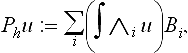
We describe in this chapter meshless methods, which use weighted finite element subspaces. For example, a solution of (11.1) is approximated by
where w is a fixed positive function, which vanishes on ∂D, and S is a suitable linear space. Such weighted approximations were already suggested by Kantorovich [32]. They have become particularly successful in connection with Rvachev’s R-functions method (cf. the survey [40] for an overview), which automatizes the construction of weight functions. The use of B-splines as basis for S suggests itself and was considered, e.g., in [46,41]. With appropriate modifications [26], the resulting finite element subspaces possess all the standard approximation properties. Numerical solutions can be computed very efficiently, in particular with the aid of software for manipulating B-splines [9] and tools from geometric modeling [17,18,30].
We use the following notational conventions. Dependencies on parameters are not always indicated, if they are clear from the context. For example, bk = bnk,h denotes the tensor product B-spline defined in Subsection 11.2.1. Moreover, we write ![]() , if f ≤ cg with a constant c, which does not depend on the grid width h, indices, or arguments of functions. The symbols
, if f ≤ cg with a constant c, which does not depend on the grid width h, indices, or arguments of functions. The symbols ![]() and
and ![]() are defined analogously. Finally, || || denotes the 2-norm for vectors and matrices and
are defined analogously. Finally, || || denotes the 2-norm for vectors and matrices and
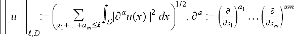
the norm on the Sobolev spaces H![]() (D) [1]. We assume throughout that the boundary ∂D is piecewise smooth and has the cone property, i.e., there are no cusp-like singularities.
(D) [1]. We assume throughout that the boundary ∂D is piecewise smooth and has the cone property, i.e., there are no cusp-like singularities.
11.2 SPLINES ON UNIFORM GRIDS
Uniform splines, discussed in this section, are spanned by scaled translates of a single B-spline (cf. chapter 6 by C. de Boor). Algorithms are particularly efficient and elegant, and there are a number of beautiful theoretical results originating from the classical work of Schoenberg [43] (cf. also [10] and chapter 10 by H. Prautzsch and W. Böhm).
Unlike for univariate splines, general knot sequences do not permit local refinement in several variables. Hence, from a practical point of view, there is not a very significant advantage over uniform knots. Adaptive refinement is possible in both cases with the aid of hierarchical bases and wavelet constructions.
11.2.1 Uniform B-splines
Uniform B-splines are special cases of the general B-splines Bk,n,t, described in chapter 6 by C. de Boor, and correspond to the uniform knot sequence t = …, -h, 0, h, …. They are scaled translates of the standard cardinal B-spline, which can be constructed with a particularly simple averaging process.
11.2.1 Definition
The standard uniform B-spline of order n > 1 is defined by the recursion
starting with the characteristic function b1 of the unit interval [0, 1).
With the first averaging step, we obtain the piecewise linear hat-function b2, which equals 1 at x = 1 and vanishes outside (0, 2). One more average yields the piecewise quadratic B-spline b3 with support (0, 3). In general, bn is a positive piecewise polynomial of degree < n, which is (n − 2)-times continuously differentiable at the integers and vanishes outside (0, n).
Forming products of uniform B-splines, we obtain multivariate B-splines on tensor product grids.
11.2.2 Definition
A normalized uniform m-variate B-spline of order n, grid width h, and shift k = (k1, …,km) ∈ Zm is defined by
As is illustrated in Figure 11.1, the B-spline bk is a scaled and translated normalized univariate B-spline in each coordinate direction. In particular, bk has support

and is a polynomial of coordinate degree < n on each grid cell Q = lh + Q*h. The normalizing factor h-m/2 ensures that the B-splines are uniformly bounded with respect to the L2-norm, i.e.,
More generally, ||bk||![]()
![]() h-l for l
h-l for l ![]() < n. This normalization is particularly convenient for finite element applications, so that we prefer it to the standard choice of simple scaling in this context.
< n. This normalization is particularly convenient for finite element applications, so that we prefer it to the standard choice of simple scaling in this context.
11.2.2 Splines on bounded domains
Splines are linear combinations of B-splines. The following more precise definition will be used for constructing finite element subspaces in the next section.
11.2.3 Definition
The splines S(D) consist of the linear combinations
where the sum is taken over all relevant shifts k, i.e., all k, for which bk has some support in D.
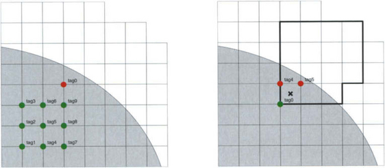
Definition 11.2.3 is illustrated in Figure 11.2 for quadratic splines (n = 3), where we have marked the lower left corners kh, k ∈ K, of the supports of the relevant B-splines. Apparently, depending on the shape of the domain D, the set of relevant shifts k may be complicated to describe explicitly. Therefore, in the implementation of algorithms, we will always allocate storage for an m-dimensional array of coefficients and simply mark the positions corresponding to the relevant shifts k ∈ K. This is much more efficient than storing precise lists.
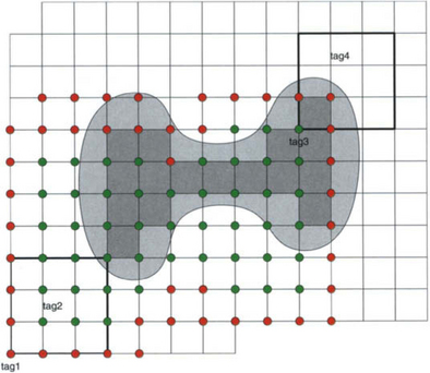
Figure 11.2 Relevant B-splines bk, spanning S(D), and classification into inner B-splines bi and outer B-splines bj.
It is important to note that the B-spline basis for S(D) is not uniformly stable with respect to the grid width h. This is due to the outer B-splines
(marked with red dots in Figure 11.2), for which no grid cell in their support is completely contained in D. The distinction between outer and inner B-splines
(marked with green dots in the Figure), which have at least one grid cell in D, will be essential for stabilizing the basis (cf. Subsection 11.3.2).
Splines have the local approximation power of polynomials, as stated in the following basic error estimate [44].
11.2.3 Hierarchical bases
To resolve small geometric details or rapid changes in solutions, local grid refinement is essential. There are numerous techniques, in particular in connection with wavelets (cf. chapter 14 by L. Kobbelt). As an example, we describe an elementary strategy for hierarchical subdivision of B-splines. This technique is very easy to implement and well suited for spline-based finite element approximations.
The hierarchical B-spline basis corresponds to a nested sequence of domains Dv, which specifies where the grid should be refined. The following natural selection of the basis functions, based on the standard subdivision schemes for splines [8,15], was proposed in [34].
11.2.4 Definition
The hierarchical spline space S(D), corresponding to the domains
is spanned by the B-splines
where Kv denotes the shifts k, for which D ∩ supp bk,hv is a nonempty subset of Dv, but is not contained in Dv+1.
This definition can be interpreted in the following way. We select a subset of the relevant B-splines for D with grid width h and replace it by B-splines of grid width h/2 via subdivision. From the B-splines on the finer grid, again, a subset is selected and refined. This process is repeated according to the sequence of domains Dv.
It is easily checked that the B-splines, spanning S(D), are linearly independent. If
we can show inductively, for v = 0, 1, …, that the coefficients ck,v are zero. First, we restrict x to the open set ![]() . By Definition 11.2.4, all B-splines with grid width hv, v > 0, vanish on this set. On the other hand, for each B-spline bk,h0, k ∈ K0, there exists a point x ∈ D0,1, where this B-spline is nonzero. Hence, by the local linear independence of the B-splines corresponding to one grid, all coefficients ck,0 must be zero. Now, we repeat the argument, restricting x successively to the sets D1,2, D2,3, ….
. By Definition 11.2.4, all B-splines with grid width hv, v > 0, vanish on this set. On the other hand, for each B-spline bk,h0, k ∈ K0, there exists a point x ∈ D0,1, where this B-spline is nonzero. Hence, by the local linear independence of the B-splines corresponding to one grid, all coefficients ck,0 must be zero. Now, we repeat the argument, restricting x successively to the sets D1,2, D2,3, ….
The hierarchical spline space S(D) contains for each domain Dv all B-splines bk,hv, for which the portion of their support in D is completely contained in Dv. Either such a B-spline belongs to the hierarchical basis, or, if D ∩ supp bk,hv ⊂ Dv+1, it can be represented as a linear combination of B-splines with smaller grid width via subdivision. Hence, as is to be expected, the local approximation power of S(D) corresponds to the level of refinement.
Figure 11.3 illustrates Definition 11.2.4 for bilinear splines with 3 grids. The subdomains D2 ⊂ D1 ⊂ D0 = D are displayed with different gray levels, and the lower left corners of the supports
of the B-splines in the basis are marked according to their level. For example, a blue/green dot corresponds to two B-splines with grid-widths h0 and h1 = h0/2, respectively.
11.3 FINITE ELEMENT BASES
In this section, we describe several types of weighted finite element subspaces, as proposed, e.g., in [40,46,26]. The essential difference, compared to standard mesh-based subspaces, is the treatment of boundary conditions. These are incorporated via weight functions, so that no mesh generation is required. As a result, we obtain finite elements on uniform grids, which share all the computational advantages of B-spline representations.
11.3.1 Mesh-based elements
Most of the standard finite element bases are constructed using a mesh of the domain. Figure 11.4 gives examples of triangular meshes in two and three dimensions, constructed with the ART-algorithm of A. Fuchs [20,21]. This method uses a physically motivated optimization strategy to achieve an almost regular mesh structure, i.e., almost all interior vertices have the same number of neighbors.
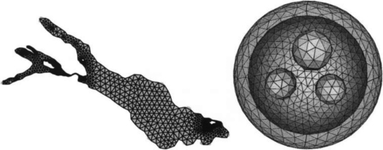
Generating finite element meshes is often the bottleneck in finite element simulations. Especially for three-dimensional problems, the construction of meshes with good geometric properties is a highly nontrivial task. Among the many algorithms, which have been developed, one can distinguish between three major approaches: advancing front techniques, domain decomposition and Delaunay triangulations. All methods have their pros and cons and, which one to choose, depends very much on the particular application.
The construction of finite element bases with respect to a given mesh is straightforward, at least if no continuous derivatives are required. Figure 11.5 lists some commonly used elements for triangular meshes. They are described in terms of the parameters which define the finite element approximation on a single triangle. For example, the standard linear element (degree 1) is determined by the 3 values at the vertices (dimension 3), indicated by dots. The corresponding piecewise linear approximations are continuous, hence belong to H1. Higher order elements can be defined by specifying more interpolation points, which are arranged in a regular triangular array. The quadratic case is shown in the Figure. To construct elements which join continuously differentiable across edges is more difficult. A classical example of a H2-element is Argyris′ triangle. It has degree 5 (dimension 21) and is determined by specifying values, first, and second derivatives at the corners (marked with dots, small, and large circles) and normal derivatives at the midpoints of the edges (marked with orthogonal bars). An alternative is the Clough-Tocher macro-element, which achieves H2-smoothness with degree 3 by splitting the triangle at the centroid.
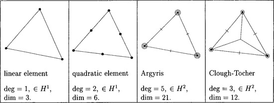
Figure 11.5 shows only a very small selection of the available possibilities. We refer to [12,50] for other examples and for quadrilateral and trivariate elements. No attempt is made here to analyze mesh-based elements in more detail. The brief description was included merely for comparison purposes. As is apparent from the bivariate examples given in the Figure, higher order or smooth elements require many parameters. In contrast, elements constructed with B-splines, as discussed in the next subsection, yield smooth highly accurate approximations with relatively few parameters. Moreover, no mesh generation is necessary, so that computing times are significantly reduced.
11.3.2 WEB-basis
At first sight, the use of B-splines as finite element basis functions seems not feasible, because the uniform grid does not conform to the boundary. However, this difficulty is easily overcome. To satisfy essential homogeneous boundary conditions, we multiply with a positive weight function w, which vanishes on ∂D, i.e., we approximate with the space
spanned by weighted relevant B-splines. For example, for a smooth domain, we may use a weight function, which is equivalent to the distance to the boundary, i.e.
There are a number of other possibilities, in particular for domains, which can be described in terms of simple primitives (lines, planes, circles, cylinders, etc.). A systematic approach will be discussed in the next subsection.
As we already remarked in Subsection 11.2.2, the B-spline basis is not uniformly stable when restricted to D. This may lead, e.g., to excessively large condition numbers of finite element systems. A well conditioned basis can be constructed with the aid of the classification of the relevant B-splines bk for the domain D into inner and outer B-splines (cf. Figure 11.2). To stabilize the basis, the outer B-splines bj, for which, by definition, no mesh cell of their support is contained in D, are attached to the inner B-splines bi. This has to be done in such a way, that polynomial precision, which guarantees full approximation order, is preserved. Hence, let us consider the B-spline representation
of a polynomial p of order n on D. As is well-known, q is a polynomial of the same order as p (cf., e.g., [10] for a proof in a more general context). Therefore, we can compute any coefficient q(j), j ∈ J, from nm coefficients q(i), corresponding to an array of shifts
closest to j. To compute q(j), we interpolate the values q(i) at the shifts in and evaluate the interpolant at j. Hence, if
denotes the value at j of the Lagrange polynomial associated with i ∈ I(j), we have
Inserting the expression for q(j) into (11.5) and interchanging sums gives
where J(i) ⊂ J is the set of all shifts j, for which i ∈ I(j). This identity suggests to define the term in square brackets as the proper extension of the inner B-spline bi. Of course, we have to multiply by the weight function w and choose an appropriate normalization. These considerations led to the following definition [26] (cf. also http://www.web-spline.de).
11.3.1 Definition
The weighted extended B-splines (web-splines)
with xi the center of an interior grid cell Qi ⊂ D in the support of bi form a basis for the web-space Swe.
Not all finite element simulations require subspaces that conform to boundary conditions. If no weight function is used, we denote the span of the extended B-splines by Se. Formally, this corresponds to the case w ≡ 1 in Definition 11.3.1.
Figure 11.6 illustrates the construction of the web-basis for quadratic splines (n = 3). On the left-hand side, the values of the coefficients ei,j with i ∈ I(j) are given for an outer B-spline bj. They are associated with the lower left corners of the supports of the inner B-splines bi. The zeros in the first and second column indicate that this outer B-spline is actually involved only in 3 web-splines Bi. This is because j1 = i1 for the right column of the shifts i ∈ I(j), causing the Lagrange polynomials associated with the other shifts in I(j) to vanish at j. On the right-hand side, the support of a web-spline Bi is shown together with the coefficients ei,j of the adjoined outer B-splines bj, j ∈ J(i). The point xi is marked by a cross.
11.3.3 R-functions
Many simple domains admit ad-hoc definitions of weight functions w. For example, for an annulus with radii 1 and 2, we may set
However, multiplying functions of implicit equations for boundary curves is not always possible. If we define
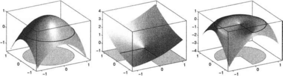
for the domain on the right of Figure 11.7, all functions in the finite element space Sw vanish on the coordinate axes. This imposes an undesirable constraint on the approximations. Fortunately, there exists a systematic approach, based on Rvachev’s concept of R-functions (cf., e.g., [40,45]). We describe below a special case of this fairly general theory, which is adequate for illustration purposes.
11.3.2 Definition
A function r : ![]()
![]() →
→ ![]() is an R-function, if its sign depends only on the sign of its arguments.
is an R-function, if its sign depends only on the sign of its arguments.
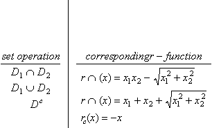
R-functions are closely related to Boolean functions. In fact, for any Boolean set operation o there exist associated R-functions ro, which define the corresponding operation on weight functions. In other words, if wv is a weight function for a set Dv, then
is a weight function for D1 ![]() D2. A popular choice of associated R-functions is shown in the following table.
D2. A popular choice of associated R-functions is shown in the following table.
Returning to the discussion of the domain
with f2(x) = x1 and f3(x) = x2, we can define
as is illustrated in Figure 11.7. The function f1 is depicted on the left, r∪(f2(x), f3(x)) in the middle, and finally w on the right of the Figure.
The explicit form of the weight function can be complicated. However, for computations this is irrelevant. Evaluation and differentiation is performed using the algorithmic definition with the aid of automatic differentiation [37,24]. The procedure is similar to algorithms in constructive solid geometry.
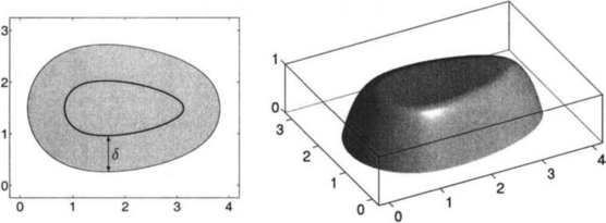
For general domains, described, e.g., by NURBS-representations [30,19], numerical techniques have to be used. A straightforward construction of a weight function is illustrated in Figure 11.8. The distance function is used near the boundary, where it is free of singularities, and blended smoothly with a plateau inside the domain. More precisely, we define
where δ controls the size of the plateau and γ the smoothness. The plateau facilitates the use of precomputed values when assembling finite element matrices. However, it should not be chosen too large in order to keep the derivatives of the weight function small.
As is apparent from the above examples, there is a great deal of flexibility in the construction of weight functions. In particular, spline approximations and numerical techniques can be effectively combined with the R-functions method.
11.3.4 Stability
With appropriate normalization, the norm of a finite element approximation is equivalent to the corresponding norm of the coefficients of the basis functions. This important stability property is also valid for the web-spaces Swe under mild assumptions on the weight function. For example, we may require that w is smooth and
Essentially, this condition implies that the norm of the gradient vanishes with one order less at the boundary than the weight function. It is valid for powers of the weight function (11.6) and also for products of such weight functions, constructed from distance functions to different boundary segments. Of course, (11.7) also holds for the trivial weight function w ≡ 1 formally corresponding to the spaces Se.
Stability can be proven with the aid of dual functions λ![]() , which are biorthogonal to the B-splines bi and uniformly bounded,
, which are biorthogonal to the B-splines bi and uniformly bounded,
There is a great deal of flexibility in the construction of such dual functions. In particular, we may require that the support of λ![]() is contained in the subcell
is contained in the subcell
of the grid cell Q![]() ⊂ supp b
⊂ supp b![]() ∩ D.
∩ D.
We claim that (11.8) remains valid if we replace bi by the web-splines Bi and λ![]() by the weighted dual functions
by the weighted dual functions
The biorthogonality follows easily since none of the outer B-splines bj has support on any of the grid cells Q![]() ⊂ D. By Definition 11.3.1, this implies
⊂ D. By Definition 11.3.1, this implies
and therefore
For the uniform boundedness we observe that
so that ![]() . The first inequality follows from the assumption (11.7), noting that for any point y on the line segment between x
. The first inequality follows from the assumption (11.7), noting that for any point y on the line segment between x![]() and x
and x
since x lies in a subcell of the grid cell Q ![]() ⊂ D.
⊂ D.
Similarly, we can show that ![]() for
for ![]() = 0, 1. In view of the local support of the web-splines and the dual functions, this implies the following stability result.
= 0, 1. In view of the local support of the web-splines and the dual functions, this implies the following stability result.
11.3.1 Theorem
For any linear combination uh = ∑i∈I uiBi of web-splines with coefficient vector U,
We emphasize that this Theorem is in general false for the spaces S and Sw, spanned by B-splines and weighted B-splines, respectively. For these spaces, the instability of the basis may lead to excessively large condition numbers of Galerkin systems and very slow convergence rates for iterative methods.
11.4 APPROXIMATION OF BOUNDARY VALUE PROBLEMS
Using weighted spline spaces, elliptic boundary value problems can be approximated in a familiar fashion [12]. We illustrate this by considering several typical model problems. In particular, the treatment of different types of boundary conditions is discussed since this affects the construction of the finite element subspaces. Finally, we state a basic error estimate and sketch the implementation of spline-based finite element techniques.
11.4.1 Essential boundary conditions
Essential boundary conditions have to be incorporated in the finite element subspaces since they are not automatically satisfied by solutions of appropriate variational problems. As a model problem, we consider the Poisson equation with homogeneous Dirichlet boundary conditions (11.1), mentioned in the introduction. We can construct approximations
choosing either one of the spaces Sw(D), Swe(D), or the weighted hierarchical spline space Sw(D) as finite element subspace Vh. Both the minimization of the functional (11.2) and the equations (11.3) with V replaced by Vh lead to the finite element equations
for the vector U of coefficients ui.
Figure 11.9 shows on the left the solution of (11.1) with f ≡ 1 on a circular domain with 3 holes, representing, e.g., the displacement of a membrane with constant load. Numerical approximations were computed with the web-spaces Swe and, for comparison, also with hat-functions on a triangulation of the domain. For orders 2, 3, 4, 5, 6 (markers *, •, ![]() ,
, ![]() ,
, ![]() , respectively), the diagram on the right shows the L2-error versus the number of basis functions. Compared to hat-functions (
, respectively), the diagram on the right shows the L2-error versus the number of basis functions. Compared to hat-functions (![]() marker), web-splines yield highly accurate solutions. For example, with 496 web-splines of order 4 the relative error in the L2-norm
marker), web-splines yield highly accurate solutions. For example, with 496 web-splines of order 4 the relative error in the L2-norm ![]() is 9.1705e-05 (in the H1-norm 7.8161e-04) whereas 17602 standard finite elements are needed to achieve a relative L2-error of 5.1614e-04.
is 9.1705e-05 (in the H1-norm 7.8161e-04) whereas 17602 standard finite elements are needed to achieve a relative L2-error of 5.1614e-04.
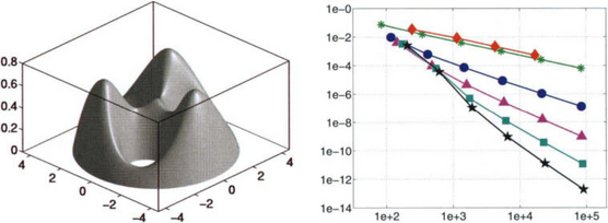
Figure 11.9 Displacement (magnified) of a membrane with constant load and error of piecewise linear and web-spline approximations of order n = 2,…, 6.
The Galerkin matrix Gwe for the space Swe can be computed with simple row and column operations from the larger matrix Gw for Sw. More precisely, Gwe = PGwPt with pi,j = (δi,j + ei,j)/w(xi), as is apparent from Definition 11.3.1. The transformation P, corresponding to the stabilization of the weighted B-spline basis, substantially reduces the condition number of the Galerkin system. In the example in Figure 11.9,
for h = 0.35 and bilinear splines (n = 2). The size of the system is reduced from 496 to 351 variables. For smaller grid width and splines of higher order, the difference is even more dramatic. For example, for h = 0.0875 and n = 5, the condition estimate of MATLAB [25] yields cond∞(Gw) = 9.3315e+61, while the condition of the reduced system is 3.0532e+10. This shows that the parameter reduction by the transformation P significantly improves the stability of the Galerkin system, thus permitting more accurate solutions and better convergence rates of iterative solvers.
Of course, Galerkin’s method applies to equations with variable coefficients as well. It is sufficient to assume that the boundary value problem can be described by the variational equations
where a and 〈f, ˙〉 are continuous bilinear and linear forms on H01(D) and a is elliptic, i.e.
(cf. [12] for several examples). The Lax-Milgram Lemma implies existence and uniqueness of weak solutions in this very general setting. Again, the finite element approximation uh ∈ Vh is obtained by replacing V by Vh in (11.10).
Problems with prescribed boundary data, u = g on ∂D, can be treated as well. They are reduced to the homogeneous case via the substitution u =: v + ![]() , where
, where ![]() is an extension of g to all of D. In effect, we seek an approximation for u from the affine space
is an extension of g to all of D. In effect, we seek an approximation for u from the affine space ![]() + Vh.
+ Vh.
11.4.2 Natural boundary conditions
As a typical problem, we consider the Laplace equation with Neumann boundary conditions,
assuming that the compatibility condition ∫∂D g = 0 is satisfied. The weak formulation of (11.11) is
Since no boundary conditions are imposed on the test functions v, the finite element formulation is much simpler than for problems with essential boundary conditions. No weight function is required, and we can work with the spline spaces S or Se.
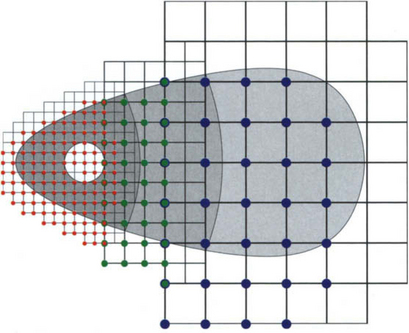
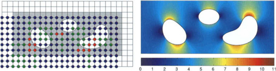
As an example, Figure 11.10 illustrates the computation of incompressible flow through a channel with three obstacles. In this case, u is the potential and –grad u the velocity. On the right of the Figure, we visualize ||grad u || for constant flow rate at the in- and outlet of the channel (∂u/∂n = ±v0 on the vertical boundaries). The finite element solution uh was calculated with extended B-splines of order 4 (uh ∈ Se). As for essential boundary conditions, the results are much superior to mesh-based approximations. For 9709 basis functions the relative L2-error is 2.2499e-08, which is by a factor 35290 smaller than for an approximation with 9835 hat-functions and a triangulation with mesh width 1/16. Moreover, as shown on the left of Figure 11.10, to construct the basis for Se, only very few B-splines have to be extended. For most of the inner shifts (marked with blue dots) the web-splines Bi coincide with the standard B-splines bi.
The more general Neumann problem,
with a(x), b(x) > 0, can be approximated in a completely analogous fashion. The variational form is
and we can use any of the spaces S(D), Se(D), or S(D) to compute finite element approximations.
11.4.3 Mixed and higher order boundary conditions
As an example of a mixed problem, we consider the system of linear elasticity
with the boundary conditions
where γ has positive (m − l)-dimensional measure. This system determines the displacement (u1(x), u2(x), u3(x)) of a three-dimensional elastic body, fixed at Γ, under a volume force with density f and a force applied to ∂DΓ with density g. The constants λ and μ are the Lamé coefficients, the matrix σ is the stress tensor, and ξ denotes the outward boundary normal. Without going into details, minimizing the potential energy over
yields a natural variational formulation. Hence, if wΓ is a weight function equivalent to the distance to Γ, each of the spaces
can be used to construct finite element approximations. An example is shown in Figure 11.11, where an elastic structure is attached to a planar surface Γ = {x : x1 = 0}. Here, the obvious choice wΓ(x) = x1 yields very simple weighted finite element subspaces. Higher order boundary conditions arise, e.g., in the biharmonic problem,
For homogeneous boundary conditions (g0 = g1 = 0), (11.12) describes the equilibrium position of a clamped plate under the action of a transverse force. In this case, finite elements should vanish to second order at the boundary. Hence, we choose a weight function, which, for smooth boundaries, is equivalent to the square of the distance function. For example, if D is the unit disc,
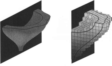
Figure 11.11 B-spline grid for computing the deformation of an elastic structure, fixed at a planar surface.
We can also use the weight function to construct affine finite element subspaces, which satisfy the inhomogeneous boundary conditions. If w = w12 and ∂w1/∂n = −1 on the boundary, as in the above example, then
where ![]() denotes an extension of ψ to D, satisfies the boundary conditions. Hence, each of the affine spaces
denotes an extension of ψ to D, satisfies the boundary conditions. Hence, each of the affine spaces
provides admissible approximations.
11.4.4 Error estimates
For most elliptic boundary value problems, the order of convergence of finite element approximations is determined by the order of the basis functions. Essentially, this is also true for all spline spaces described in section 11.3. For the norm associated with the variational formulation, the arguments are particularly simple and familiar from classical finite element analysis [48],[12]. As an illustration, we consider the Dirichlet problem for Poisson’s equation, discussed in Subsection 11.4.1. The generalization to the abstract variational problem (11.10) is straightforward.
11.4.1 Theorem
If uh is a finite element approximation to a solution u of (11.1) from a linear subspace Vh ⊂ H01(D), then
This estimate is a direct consequence of the variational formulation. By (11.9), uh = ∑iuiBi satisfies
Combining this with (11.3) yields ∫ grad (u - uh) grad v = 0 for all v ∈ Vh. Hence, choosing v := uh - vh,
where the left-hand side is ![]() by Friedrich’s inequality, and the right-hand side is
by Friedrich’s inequality, and the right-hand side is ![]() . Dividing by ||u - uh||1, the Theorem follows.
. Dividing by ||u - uh||1, the Theorem follows.
11.4.1 Theorem
implies convergence of the finite element approximations from Swe and therefore also from the larger space Sw. Moreover, with the aid of the canonical projector
associated with the dual functions for the web-basis, we can derive the following standard error bound [26,27].
11.4.2 Theorem
If the weight function w satisfies (11.7) and the solution u as well as u/w are smooth, then
for finite element approximations uh from Swe.
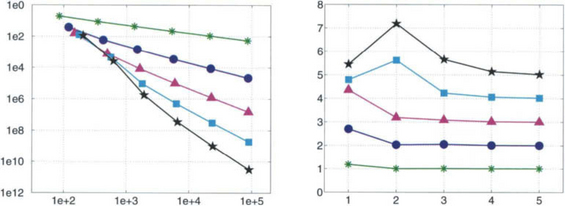
As shown in Figure 11.12 the numerical results for the model problem (11.1) live up to the theoretical predictions. For the example considered in Figure 11.9 the H1-error is plotted versus the number of web-splines on the left-hand side. The right-hand side shows the ratio between consecutive logarithmic errors in order to make the rate of convergence apparent. As is to be expected, the use of higher order approximations pays off.
11.4.5 Implementation
A typical finite element simulation with splines consists of the following major steps:
Each of these components will now be described in turn. For simplicity, we consider only the spaces S(D), Sw(D), and Swe(D), which do not involve adaptive refinement.
Construction of the basis.: The domain is enclosed in a bounding box and covered by a regular grid. Then the grid cells are classified into interior, boundary, and exterior cells (cf. Figure 11.2). This minimal information is sufficient to determine all parameters for constructing the various bases. Among all B-splines b![]() with support overlapping the bounding box, we mark the inner B-splines bi and the outer B-splines bj, checking whether their support contains at least one interior grid cell Qi or merely boundary cells. The union of these B-splines, bk, k ∈ K = I ∪ J, forms a basis for S.
with support overlapping the bounding box, we mark the inner B-splines bi and the outer B-splines bj, checking whether their support contains at least one interior grid cell Qi or merely boundary cells. The union of these B-splines, bk, k ∈ K = I ∪ J, forms a basis for S.
To construct the web-basis Bi for Se, we first determine for each j ∈ J the closest array I(j) among the inner shifts i. Then we associate with each i the set J(i) and the coefficients ei,j. Since ei,j, i ∈ I(j), only depend on the relative position of the array I(j) with respect to the outer shift j, and I(j) is usually close to j, tabulated values can be used in most cases.
For the spaces Sw and Swe, we have to specify the weight function. If permitted by the description of D, the R-functions method can be used, and the weight function w is specified explicitly via an algorithmic expression. In general, w has to be constructed with the aid of distance functions and must be evaluated numerically.
Assembly of the finite element system.: For the entries of the finite element matrices we have to compute integrals over grid cells with integrands that involve values and derivatives of the weight function, B-splines, and functions occurring in the formulation of the boundary value problem. Good results are usually obtained with tensor product Gauβ formulas. For interior grid cells, the integration is straightforward. However, boundary grid cells have to be divided into subcells, which can be mapped smoothly to standard domains. Integrating directly would result in a loss of accuracy due to the non-smooth boundary of the intersections Q ∩ D. While the subdivision in two dimensions just requires cuts by straight lines (cf., e.g., [42]), in three dimensions a number of different possibilities have to be considered; Figure 11.13 shows a few typical examples. To facilitate the visualization of the subdivision, arrows indicate the transformation to standard integration areas.

The integrands can be evaluated efficiently. The most complicated part is computing derivatives of the weight function at the Gauβ points. If w is defined via R-functions, automatic differentiation can be used in conjunction with the algorithmic definition [24],[47]. The numerical evaluation of w involves Newton’s method. However, only very few iterations are necessary since for neighboring points good start values exist. Moreover, for weight functions with plateau, the additional computational effort is required only near the boundary.
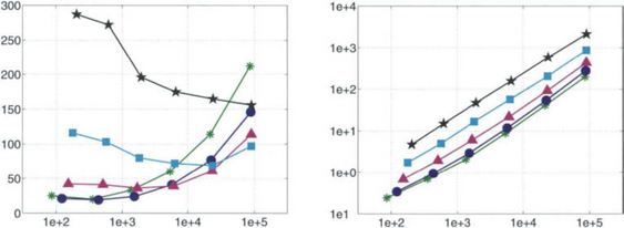
Iterative Solution.: The finite element systems can be solved with any of the standard iterative schemes. For example, as is illustrated in Figure 11.14, conjugate gradients, preconditioned with SSOR, give very good results. For the Dirichlet problem, considered in Figure 11.9, we have plotted on the left-hand side the number of iterations versus the dimension of the spline space Swe. The diagram on the right-hand side shows the total computing time in seconds, measured on a Pentium 11/400 MHz class personal computer. There is only a fairly moderate growth in the required computational work. Systems with more than 600,000 unknowns could be handled without any stability problems.
The spline approximations on uniform grids are also ideally suited for multigrid techniques. Subdivision algorithms [8,15] and the standard projector (11.13) provide natural grid transfer operators. For the standard multigrid w-cycle optimal grid independent convergence rates can be established [28]. Hence, the solution time remains proportional to the dimension of the spline spaces. Such techniques are particularly important for large scale three-dimensional applications.
11.5 SUMMARY
Weighted spline approximations provide a natural link from geometric modeling to finite element simulation. They do not require any grid generation, thereby eliminating an often time-consuming preprocessing step. Moreover, software for manipulating B-splines can be used to assemble Galerkin matrices and to visualize numerical results. Unlike for mesh-based methods, there are no limitations on the smoothness of the basis. Therefore, highly accurate approximations are possible with relatively few parameters.
An important feature of weighted finite elements is the simplicity of the geometry description. For domains defined in terms of implicit equations, the associated weight functions can be constructed with the R-functions method. This technique is applicable to many engineering problems, in particular those involving constructive solid geometry models. Efficient algorithms are also available for general NURBS-domains, where weight functions have to be constructed numerically. Hence, the methods combine well with standard boundary representations in CAD-systems.
Acknowledgement.
I am very grateful to Joachim Wipper for extensive numerical computations. Moreover, I would like to thank Alexander Fuchs and Jörg Hörner for helping with comparisons of spline- and mesh-based methods.
1. Adams, R.A. Sobolev Spaces. Academic Press; 1978.
2. Argyris, J.H. Energy Theorems and Structural Analysis. Butterworths; 1960.
3. Argyris, J.H. Recent Advances in Matrix Methods of Structural Analysis. London: Pergamon Press; 1964.
4. Babuška, I. The finite element method with penalty. Mathematics of Computation. 1973;27(122):221–228.
5. Babušska, I. The finite element method with Lagrangian multipliers. Numer. Math. 1973;20:179–192.
6. Belytschko, T., Krongauz, Y., Organ, D., Fleming, M., Krysl, P. Meshless methods: An overview and recent developments. Comput. Methods Appl. Mech. Eng. 1996;139(1–4):3–37.
7. Bochev, P., Gunzburger, M. Finite element methods of least squares type. SIAM Review. 1998;40:789–837.
8. Böhm, W. Inserting new knots into B-spline curves. Computer-Aided Design. 1980;12:199–201.
9. de Boor, C., A Practical Guide to Splines. Springer-Verlag: Elmsford, N.Y., 1978.
10. de Boor, C., Höllig, K., Riemenschneider, S., Box Splines. Springer-Verlag, 1993.
11. Heft 81, SPB Bubnow, I.G., Rezension über die mit dem Schurawski-Preis ausgezeichneten Abhandlungen von Prof. Timoschenko, Sammlung des Instituts für Vekehrswesen, 1913.
12. Ciarlet, P.G. The Finite Element Method for Elliptic Problems. North-Holland; 1978.
13. Ciarlet P.G., Lions J.P., eds. Handbook of Numerical Analysis. Amsterdam: North Holland, 1991.
14. Clough, R.W., The finite element method in plane stress analysis. Proc. 2nd ASCE Conf. on Electronic Computation. Pittsburgh. 1960.
15. Cohen, E., Lyche, T., Riesenfeld, R., Discrete B-splines and subdivision techniques in computer- aidedgeometric design and computer graphics. Computer Graphics Image Proc., 1980;14:87–111.
16. Courant, R. Variational methods for the solution of problems of equilibrium and vibrations. Bull. Amer. Math. Soc. 1943;49:1–23.
17. Farin G.E., ed. Geometric Modeling: Algorithms and New Trends. Amsterdam: SIAM, 1987.
18. Farin, G.E. Curves and Surfaces for Computer Aided Geometric Design. Academic Press; 1988.
19. Farin G.E., ed. NURBS for Curve and Surface Design. SIAM, 1991.
20. Fuchs, A. Almost regular Delaunay-triangulations. Internat. J. Numer. Meths. Eng. 1997;40:4595–4610.
21. Fuchs, A. Optimierte Delaunay-Triangulierungen zur Vernetzung getrimmter NURBS-Körper. PhD thesis, Universität Stuttgart. 1999.
22. Fuchs, A. Almost regular triangulations of trimmed NURBS-solids. Engineering with Computers. 2001;17:55–65.
23. Galerkin, B.G. Stäbe und Platten; Reihen in gewissen Gleichgewichtsproblemen elastischer Stäbe und Platten. Vestnik der Ingenieure. 1915;19:897–908.
24. Griewank, A., Evaluating derivatives: principles and techniques of algorithmic differentiation. Frontiers in Applied Mathematics 19. SIAM, 1999.
25. Higham, N.J., Tisseur, F. A block algorithm for matrix 1-norm estimation, with an application to 1-norm pseudospectra. SIAM J. Matrix Anal. Appl. 2000;20(4):1185–1201.
26. Höllig, K., Reif, U., Wipper, J. Weighted extended B-spline approximation of Dirichlet problems. SIAM J. Num. Anal. 2001;39:442–462.
27. Höllig, K., Reif, U., Wipper, J. Error estimates for the web-method. In: Lyche T., Schumaker L., eds. Mathematical Methods for Curves and Surfaces Oslo 2000. Vanderbilt University Press; 2000:195–209.
28. Höllig, K., Reif, U., Wipper, J. Multigrid methods with web-splines. Numer. Math. 2002;91(2):237–256.
29. Ho-Le, K. Finite element mesh generation methods: a review and classification. Computer-Aided Design. 1988;20(1):27–38.
30. Hoschek, J., Lasser, D. Fundamentals of Computer Aided Geometric Design. Nashville: A.K. Peters; 1993.
31. Huebner, K.H., Thornton, E.A., Byrom, T.G. The Finite Element Method for Engineers. John Wiley & Sons; 1994.
32. Kantorowitsch, L.W., Krylow, W.I. Näherungsmethoden der Höheren Analysis. VEB Deutscher Verlag der Wissenschaften; 1956.
33. Kardestuncer H., ed. Finite Element Handbook. Berlin: McGraw-Hill, 1987.
34. Kraft, R. Adaptive und linear unabhängige multilevel B-Splines und ihre Anwendungen. PhD thesis, Universität Stuttgart. 1998.
35. Mackerle, J. Finite Element Methods: A Guide to Information Sources. New York: Elsevier Science Publishers B.V.; 1991.
36. Owen, S.J. A survey of unstructured mesh generation technology. In: Proceedings of 7th International Meshing Roundtable. Sandia National Laboratories; 1998:239–268.
37. Rail, L.B. Automatic Differentiation. Springer Lecture Notes in Computer Science 120. 1981.
38. London Rayleigh, J.W.S., The Theory of Sound, 2nd edition. 1894, 1896.
39. Ritz, W. Über eine neue Methode zur Lösung gewisser Variationsprobleme in der Mathematischen Physik. J. reine angew. Math. 1908;135:1–61.
40. Rvachev, V.L., Sheiko, T.I. R-functions in boundary value problems in mechanics. Appl. Mech. Rev. 1995;48(4):151–188.
41. Rvachev, V.L., Sheiko, T.I., Shapiro, V., Tsukanov, I. On completeness of RFM solution structures. Comp. Mech. 2000;25:305–316.
42. Rvachev, V.L., Shevchenko, A.N., Veretel’nik, V.V. Numerical integration software for projection and projection- grid methods. Cybernetics and Systems Analysis. 1994;30:154–158.
43. Schoenberg, I.J. Contributions to the problem of approximation of equidistant data by analytic functions. Quart. Appl. Math. 1946;4:45–99. Schoenberg, I.J. Contributions to the problem of approximation of equidistant data by analytic functions. Quart. Appl. Math. 1946;4:121–141.
44. Schumaker, L.L. Spline Functions: Basic Theory. Wiley-Interscience; 1980.
45. Shapiro, V. Theory of R-functions and applications: A primer. Technical Report CPA88-3, Cornell Programmable Automation, Sibley School of Mechanical Engineering, Ithaca, NY. 1988.
46. Shapiro, V., Tsukanov, I. Meshfree simulation of deforming domains. Computer-Aided Design. 1999;31:459–471.
47. Shevchenko, A.N., Rokityanskaya, V.N. Automatic differentiation of functions of many variables. Cybernetics and Systems Analysis. 1996;32(5):139–158.
48. Strang, G., Fix, G.J. An Analysis of the Finite Element Method. Prentice-Hall; 1973.
49. Turner, M.J., Clough, R.W., Martin, H.C., Topp, L.C. Stiffness and deflection analysis of complex structures. J. Aeronaut. Sci. 1956;23(9):805–823. Turner, M.J., Clough, R.W., Martin, H.C., Topp, L.C. Stiffness and deflection analysis of complex structures. J. Aeronaut. Sci. 1956;23(9):854. []
50. Zienkiewicz, O.C., Taylor, R.I., Finite Element Method – Basic Formulation and Linear Problems, Vol. I, II, III. Butterworth & Heinemann, 2000.