
Sculptured Surface NC Machining
Many products are designed with sculptured surfaces to enhance their aesthetic appeal; it is an important factor in customer satisfaction, especially in the automotive and consumer-electronics industries. Other products have sculptured shapes to meet functional requirements, such as:
• Aerodynamic: airfoils (jet engines), impellers (compressors), marine propellers, etc.
• Optical: lamp reflectors (automobiles), shadow masks (TV monitors), radar dishes, etc.
• Medical: parts for anatomical reproduction.
• Structural: structural frames (aircraft), sporting goods, etc.
• Manufacturing: parting surfaces (molding dies), die faces (stamping dies), etc.
While these aesthetic and functional surfaces are created using CAGD (computer-aided geometric design) techniques, it is the role of SSM (sculptured surface machining) to realize them in physical form. As an ever-increasing variety of products are being designed with sculptured surfaces, efficient machining of these surfaces is becoming increasingly important in many areas of manufacturing including the automobile, consumer-electronics, aerospace, ship-building, die-making, sporting-equipment and toy-making industries. For many companies, sculptured surface machining has become a strategic technology.
22.1 INTRODUCTION
22.1.1 Overview of the sculptured surface machining process
Examples of various sculptured surface machining (SSM) processes are provided in a number of articles: airfoil machining in Mason [15], impeller machining in Takeuchi et al. [22], marine propeller machining in Choi et al. [6], die and mold machining in Altan et al. [1] and Fallbohmer et al. [12], medical parts machining in Duncan and Mair [10], etc. However, the lack of a unified framework for describing SSM processes makes it difficult to compare one approach to another.
The first step in providing such a framework is a set of basic definitions as follows:
• UMO (unit machining operation): a basic unit of an SSM operation carried out by a single cutting tool, which has a distinguishable pattern with a well-defined machining boundary.
• Machining stage: a group of UMOs employed to achieve a certain operational goal, such as roughing, finishing, clean-up, etc.
• SSM process: a set of machining stages employed in making a sculptured part.
It should be noted that the actual definitions of UMOs and machining stages may vary between different applications, but they provide a framework for representing an SSM process.
The purpose of an SSM process is to produce a sculptured part by applying a series of metal-removal processes to a workpiece. The term workpiece is used to denote the current state of the object at any given stage of the SSM process.
Most engineering disciplines are concerned with modeling. A modeling process involves abstraction and generalization, and the resulting model should serve as a general framework as well as a useful tool for investigating or solving the problem at hand. SSM process models are classified into sequential models and hierarchical models.
In the abstract, an SSM process may be viewed as a sequence of material removal functions (MRF). In the most simplistic view, the SSM process can be regarded as a ‘sculpting process’ in which a ball-endmill cutter will form the machined-surface by a series of ‘touches’, just as a sculptor forms his massif by the classical process called ‘pointing’ (Duncan and Mair [10]). Taking this view, the entire surface is treated asa single sculptured surface, and all the SSM operations are treated as a single material removal function called SCULPT. Of course, this model is too simple to be useful in metal cutting.
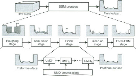
A natural extension of the sculptural model is to decompose the SCULPT operation into a number of specialized operations. If individual UMOs are used as transform functions, we will have a ‘UMO model’. If machining stages are used, a ‘machining-stage model’ may be obtained. Based on the observation that each machining stage consists of a sequence of UMOs, one may obtain a model of the SSM process, as shown in Figure 22.1, in which it is modeled as a sequence of machining stages, and each machining stage is decomposed into a sequence of UMOs.
22.1.2 Information processing issues
The SSM problem is to generate: 1) a sequence of UMOs for machining the sculptured part, 2) a sequence of NC code blocks for each UMO, and 3) cutting conditions for each NC code block. We need a separate information processing stage for each of these three steps. Given below are the three information processing stages along with their functional requirements:
1. The feature-based processing stage generates UMOs with a minimum P/M (NC programming / NC machining) ratio.
2. The geometric processing stage obtains NC blocks with the minimum cutter-failure rate and the minimum cutter-gouge rate.
3. The technological processing stage obtains cutting conditions by which maximum cutting efficiency and minimum cutting-failure rate are achieved.
Feature-based information processing
Generating an SSM process (i.e. a sequence of UMOs) from input data requires a high-level decision-making function, which in turn requires feature-based information processing. A list of machining features is extracted from the geometric definition of the design surface, and then these are converted into a sequence of UMOs (unit machining operations). The first process is called feature extraction, and the second is called computer-automated process planning (CAPP).
The main issues at this stage are 1) how to define and extract the machining features and 2) how to define and obtain the UMOs. In SSM, these two areas, feature extraction and CAPP, have not yet been fully investigated.
Geometric information processing
Geometric information processing involves the generation and verification of NC data. As shown in Figure 22.2, the generation function consists of tool path planning and cutter location data computations, while the verification function involves cutting simulation and gouge detection. To describe the geometric information processing stage, the following terms are now introduced: a CC-path is a series of cutter-contact (CC) points where the cutter is tangent to the surface being machined; and a CL-path is defined as the locus of cutter-location (CL) points, typically at the center or tip of the tool. Brief descriptions of those operations are now given:
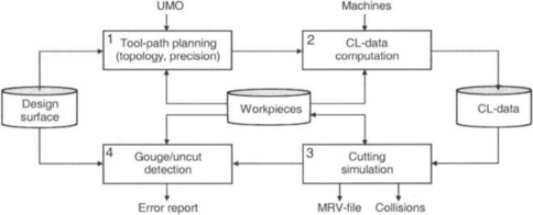
1. Tool path planning: for a UMO, CC-paths are obtained from the design surface.
2. CL-data computation: CC-paths are converted to CL-paths.
3. Cutting simulation: the workpiece is ‘virtually machined’.
4. Gouge detection: the simulated machined surface is compared against the design surface.
The cutting simulation operation also involves computing metal-removal volumes (MRV) and checking for collisions.
The key issue at this stage is how to generate dependable NC data to minimize both the cutter failure rate and cutter gouge rates, while also achieving tool path economy (i.e. minimizing the effective length of the total cutter path). Another issue is how to automate the tool path generation process by using generative NC (GNC), in order to minimize the P/M ratio.
Technological information processing
Technological information processing is mainly concerned with cutting conditions, but it also involves selecting cutting tools and choosing milling strategy options etc. Once the tool path pattern has been determined, during the geometric information processing stage, cutting efficiency is dependent on the spindle speed and feedrate for each NC block. Ideally, the feedrate would be adaptively varied according to the changes in metal removal volume. In general, the machining process conditions are affected by non-geometric factors such as:
2. Surface-finish requirements.
3. Properties of the workpiece material such as hardness, strength, ductility, etc.
4. Cutting tool material (HSS, WC, CBN, …), type, shape, etc.
5. Machine tool characteristics.
6. Milling strategy options (e.g. down-milling or up-milling, reverse-cutting or plunge-cutting, etc.)
The difficulty of technological information processing lies in the fact that there are so many variables to consider, because modern SSM operations have become so complicated. Thus, it is essential to have a cutting-condition DBMS (database management system) that is constantly updated, based on feedback from the shop floor.
22.2 UNIT MACHINING OPERATIONS
This section presents tool path topology, milling strategy options, and a comprehensive list of UMOs for 3-axis machining. Commonly used cutter types for SSM operations are the ball-endmill, flat-endmill, and round-endmill.
22.2.1 Tool path topology and milling-strategy options
Sculptured surface machining is a ‘point’ milling process in which a sequence of CC-points is traced by milling cutters. When a region is machined by the point milling method, the process is often called regional milling, and the pattern of ‘tracing’ or scanning is called the tool path topology (Marshall and Griffiths [14]). The traced region could be an area, a strip of fillets or a ‘wall’. There are four types of tool path topology pattern, as summarized below (where BC stands for boundary-curves and CPO stands for contour-parallel offset):
• Serial-pattern: xy-parallel, BC-parallel and BC-normal (Figure 22.3-a).
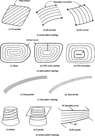
• Radial-pattern: spiral and CPO (Figure 22.3-b).
• Strip-pattern: strip-parallel and strip-normal (Figure 22.3-c).
• Contour-pattern: helical, z-constant, and BC-parallel (Figure 22.3-d).
Both the serial and radial types may be used for machining an area, and the contour type is appropriate for cutting a vertical or slanting wall. The spiral and helical topologies (Figure 3-b-1 and Figure 3-d-1) are widely used in high-speed machining. It should be noted that the so-called isoparametric tool path is a special case of the BC-parallel topology, which also includes the so-called isocurvature tool path proposed by Jensen and Anderson [13] and Suresh and Yang [21].
When planning for regional milling, it is also necessary to consider milling strategy options (Schulz and Hock [19]) and parameters related to the SSM-process such as:
22.2.2 Ball-endmill UMOs
The ball-endmill is by far the most popular cutting tool for sculptured surface machining. As shown in Figure 22.4, there are seven types of ball-endmill UMOs widely found in sculptured surface machining. Listed below are these ball-endmill UMOs together with their tool path topologies. (There are a large number of possible combinations of tool path topologies, but only the most common ones are considered here):
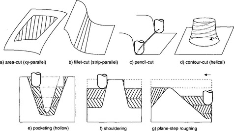
1. Area-cut: serial-pattern or radial-pattern topologies (Figure 22.4-a: xy-parallel).
2. Fillet-cut: strip-pattern topologies (Figure 22.4-b: strip-parallel).
3. Pencil-cut (Figure 22.4-c).
4. Contour-cut: contour-pattern topologies (Figure 22.4-d: helical).
5. Pocketing (hollow only): radial-pattern topologies (Figure 22.4-e).
6. Shouldering: radial-pattern or xy-parallel topologies (Figure 22.4-f).
7. Plane-step roughing (or plane-stepping): xy-parallel topologies (Figure 22.4-g).
The area-cut UMO is mainly used in generating a smooth surface by tracing the surface area. If a large ball-endmill is used during finish-machining, strips of uncut region may appear along the sharp concave fillets. These uncut regions in the concave fillets can be cleaned up by the fillet-cut UMO using a smaller ball-endmill. Since the radius of theconcave fillet is smaller than the radius of the ball-endmill, the ball-endmill will make multiple-point contact with the part surface. The trajectory of the center of the ball-endmill in this case is called a ‘pencil curve’, and the progress of the ball-endmill along the pencil-curve is called a pencil-cut UMO.
As shown in Figure 22.4-d, a ‘core-wall’ surface can be effectively machined by employing the contour-cut UMO. The remaining three UMOs in Figure 22.4 are for roughing operations: pocketing, shouldering and plane-stepping. They are based on the concept of cutting layers in which the volumes to be removed are sliced into layers by a number of (equally spaced) horizontal cutting planes. The thickness of the cutting-layer is often called the ‘plane step’, and so this type of roughing method is often called the plane-step method. Especially in pocketing, if the cavity-volume to be removed already has a cavity, as shown in Figure 22.4-e, the process is called hollow pocketing; if the cavity is to be machined from a solid stock, it is called (solid) pocketing.
22.2.3 Flat-endmill UMOs
There are seven types of 3-axis flat-endmill UMOs widely used in sculptured surface machining. They are listed below, together with their tool path topologies (but note that only the most common topologies are considered):
1. Fillet-cut (upward only): strip-normal topology (Figure 22.5-a).
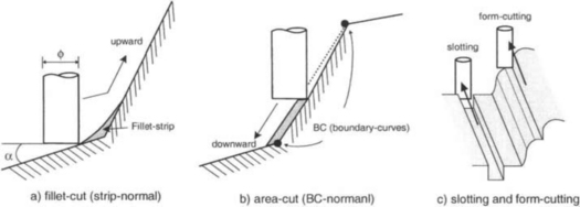
2. Area-cut (downward only): BC-normal topology (Figure 22.5-b).
5. Pocketing: radial-pattern topologies.
With 3-axis NC machine tools, flat-endmills are rarely used for finish-machining, except in the two cases shown in Figure 22.5: that is, the ‘strip-normal topology’ shown in Figure 22.5-a and the ‘BC (boundary contour)-normal topology’ shown in Figure 22.5-b. The former is often used in finish-machining of injection molding dies, and the latter is mainly employed in clean-up machining. The two ‘simple’ UMOs, slotting and 2D-contouring, are used in the roughing stage as well as in the form-cutting stage (i.e. the form-EDM stage for concave sharp edges). The other three roughing UMOs—pocketing, shouldering and plane-stepping—are defined in almost the same way as their ball-endmill counterparts.
22.3 INTERFERENCE HANDLING
Even with the most robust algorithms, there are many opportunities for making errors when generating the tool paths for sculptured surface machining (SSM). The kinds of errors considered in this section are:
1. Gouging of the part in excess of the in-tolerance value ti.
2. Collision between a non-cutting cutter element (e.g. the cutter holder) and the workpiece.
The purpose of this section is to understand the nature of cutter interference in SSM, which is essential for preventing, detecting, and correcting errors. In this section, commonly found types of cutter interference are categorized as:
1. CL-point interference: gouging occurs at a CL-point.
22.3.1 CL-point interference
Figure 22.6-a shows a typical CL-point interference; this type is known as a concave-gouge, which can occur at a CL-point located in a concave region when a cutter contacting a CC-point invades other portions of the part surface. When a smooth surface is machined with a ball-endmill, a sufficient condition for concave-gouging is given by
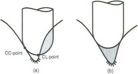
where ρ is the ball-endmill radius and kn is the maximum normal curvature. Even though some methods for preventing concave-gouging have been proposed in the literature (Choi and Jun [4]), it is not easy to detect (and correct) this type of gouging from a given tool path. Moreover, ‘correction’ of the concave-gouge would lead to a CL-point uncut as depicted in Figure 22.6-b.
22.3.2 CL-line interference
Even if there is no interference at each CL-point, a convex-gouge may occur during the movement of the tool along a CL-line, as shown in Figure 22.7-a. A convex-gouge may occur only at a CL-line (and a concave-gouge may occur only at a CL-point). Figure 22.7-a shows a typical convex-gouge associated with a ball-endmill. The ‘thickness’ of the convex-gouge (γi) is defined as the distance from the CC-point (ri) to the machined surface, and it is expressed (Choi and Jun [4]) as:
where ρ is the cutter radius, α1 = ∠r1p1p2 and α2 = ∠p1p2r2 (see Figure 22.7-a).
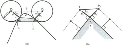
In the extreme, the convex-gouge shown in Figure 22.7-a becomes the sharp-edge gouge shown in Figure 22.7-b. In both cases (Figures 22.7-a and 22.7-b), the thickness of the convex-gouge could be unacceptably high for a large value of αi. The actual size of the convex-gouge is roughly equal to the sum of the gouge thickness γ given by (22.2) and the in-tolerance τi.
A simple way to correct (or remove) the convex gouge at pi is to insert additional CL-points at qi (for i = 1, 2), located (Choi and Jun [4]) at:
where ni is the unit normal vector at ri and c = (r2 − ri)/|r2 − r1|. Now the CL-path at the convex region is changed to the sequence
This correction is effective on both the convex-gouge of Figure 22.7-a and the sharp-edge gouge of Figure 22.7-b.
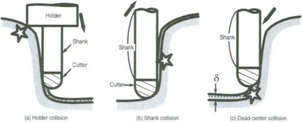
22.3.3 Collisions
A cutting tool is supposed to interact with the workpiece only through its ‘cutter-part’ (or cutting-edge), and if its non-cutting portion makes contact with the workpiece, there is a collision. In fact, there may be three types of collision: 1) holder-collisions, as shown in Figure 22.8-a, 2) shank-collisions as in Figure 22.8-b, and 3) dead-center collisions, as shown in Figure 22.8-c.
22.4 TOOL PATH GENERATION METHODS AND CONSEQUENT GEOMETRIC ISSUES
22.4.1 The conventional approach and the C-space approach The conventional approach
In CC-based TPG (tool path generation) methods, tool paths are generated by sampling a sequence of CC-points from the part surface, and then each CC-point is converted to a CL-point. Here, the part surface is used as a path-generation surface on which tool paths are generated. These are often called conventional TPG-methods.
There are three types of path planning domain in which tool path patterns are planned: the parameter domain, the guide-plane and the drive-surface. Thus, depending on the type of path-planning domain, CC-based TPG-methods can be grouped into the three cases shown in Figure 22.9:
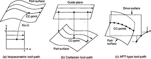
1. The isoparametric method: CC-paths are planned on the parameter domain of the part surface and then they are mapped on to the part surface (Figure 22.9-a).
2. The Cartesian method: tool paths are planned on a guide-plane and then tool positions are projected on to the part surface (Figure 22.9-b).
3. The APT (Automatically Programmed Tool) method: tool paths are defined by intersecting the part surface with a series of drive-surfaces (Figure 22.9-c).
The isoparametric method is the simplest TPG-method, but it may not be suitable for machining a compound surface consisting of a collection of surface patches. Moreover, this method is susceptible to concave gouging. Thus, the alternative Cartesian method is widely employed in modern CAD/CAM systems. The APT method has been employedin the APT system. In all these three cases, however, the CL-data computation is carried out in the following three phases:
1. Mapping: computation of a CL-point for a given ‘domain-point’.
2. Marching: finding the next domain-point from the current point on the path.
3. Side-stepping: finding the initial domain-point on the next path.
The C-space approach
The C-space (configuration space) idea has been widely used in spatial planning for robot manipulators [16] and may also be applied to NC tool path planning by treating the cutter assembly as the moving object and the workpiece and fixtures as the obstacles. The configuration of a 3-axis NC machine (i.e. its cutter) is the 3D position vector denoting a CL-point, and its C-space is given by the NC-volume VNC within reach of the cutter. In tool path planning, however, there are two types of safe C-space: ‘free-travel’ C-space and ‘machining’ C-space.
Now we will consider two CL-surfaces (SD and Sp), one from the design-surface and the other from the preform-surface, as depicted in Figure 22.10:
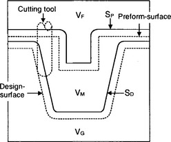
Then, as shown in Figure 22.10, the two CL-surfaces would divide the entire C-space VNC into the following three disjoint C-space volumes:
• VF : the ‘free-travel’ C-space volume (the region above SP).
• VM : the ‘machining’ C-space volume (the region between SP and SD and including both surfaces).
The geometric entities SP, SD, VF, VM, VG are called C-space elements.
As will be discussed shortly, these C-space elements contain all the geometric information needed for generating tool paths. In summary, the C-space approach to tool path generation may be formalized as follows:
1. Compute SP: CL-surface of the preform-surface.
2. Compute SD: CL-surface of the design-surface (with an uncut-allowance).
Compared with conventional methods, the key feature of the C-space approach is that all the decisions, including global ones such as feature extraction and adaptive feed control, can be based solely on the C-space representation.
22.4.2 Geometric issues in conventional approach
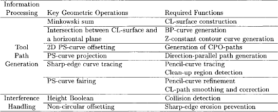
The geometric information processing of SSM may be classified into a tool path generation (TPG) step and an interference handling step in which geometric issues are identified; this is the case both in the conventional approach and in the C-space approach. Table 22.1 summarizes the geometric aspects of the conventional approach, while the six key geometric procedures in the TPG step are listed below:
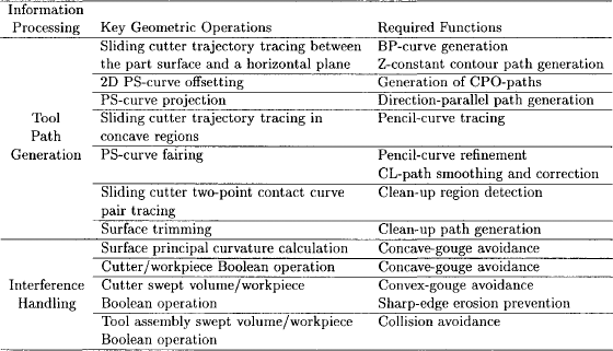
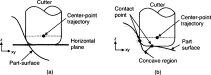
• A sliding cutter trajectory between the part surface and a horizontal plane is traced to generate a BP (boundary pocket)-curve or a z-constant contour curve. However, many researchers are still struggling to design and implement a robust tracing algorithm (see Figure 22.11-a).
• A 2D PS(point sequence)-curve offsetting algorithm is used to generate a series of contour-parallel offset (CPO) curves especially in pocket machining. A more detailed description of this issue is presented in section 22.5.2.
• PS-curves defined during tool path planning are projected on to the part surface to generate CPO-paths or direction-parallel CC-paths. Vertical and horizontal projection are usually sensitive in near-vertical and near-plane regions of the part surface respectively. Depending on the shape of the part surface, we should select an appropriate projection method, such as the normal projection.
• Sliding cutter trajectories in concave regions are traced to detect pencil-curves on the part surface. The trajectory of the center of the ball-endmill in this case is the pencil-curve (see Figure 22.11-b).
• Sliding cutter two-point contact curve pairs are traced to extract clean-up machining regions. The sliding cutter in this case is the smallest used in finish machining (see Figure 22.11-b).
• PS-curve fairing is used in refining pencil-curves and correcting CL-paths to improve the quality of the machined surface.
The following four key geometric issues are also identified in the interference handling step:
• Principal curvature calculations and Boolean operations between the cutter and the workpiece are used to detect concave-gouging (CL-point gouging) in SSM.
• Boolean operations between the volume swept by the cutter and the workpiece are used to detect convex-gouging (CL-path gouging).
• Boolean operations between the volume swept by the tool assembly and the workpiece are used to check for collisions.
In these cases, effective performance of the Boolean operations requires a unified scheme for representing the cutter and the workpiece. There is no general algorithm to prevent the erosion of sharp edges in the conventional approach, so a special algorithm has to be designed and implemented for each case.
22.4.3 Geometric issues in the C-space approach
In the C-space approach, six geometric issues may be identified in the TPG step and two more become apparent in the interference handling step. PS-curve handling algorithms, discussed in the conventional approach, can also be applied to the C-space approach. The six key geometric issues in the TPG step can be summarized as follows.
• The concept of the Minkowski sum is used to construct the inverse tool offset surface, the CL-surface. A unified scheme for consistent representation the part surface and the CL-surface is required to construct the CL-surface effectively. In section 22.5.1 an algorithm for constructing the CL-surface is described. The z-map model is used as a representation scheme for the CL-surface.
• A z-constant contour curve including a BP-curve are computed by intersecting the CL-surface and a horizontal plane. The z-constant contour curve becomes a path segment in the C-space approach.
• As in the case of the conventional approach, 2D PS-curve offsetting, PS-curve projection, and PS-curve fairing are employed to handle PS-curves (in the generation of CPO-paths, direction-parallel tool path generation, and in pencil-curve refinement).
• Since pencil-curves are represented as sharp-edges in the CL-surface, we use the algorithm for tracing sharp-edge curves to detect pencil-curves and clean-up regions in the C-space approach.
The C-space of the tool assembly is constructed from the part surface using the concept of the Minkowski sum. Collisions between the part surface and the tool assembly are easily detected using height Boolean operations, because the tool assembly is represented as a line segment in its C-space. To prevent sharp-edge erosion in the C-space approach, we must use a special method, such as a non-circular offsetting of the sharp edges. (If a cutter moves along a circular offset tool path which crosses a convex sharp edge, the cutter contacts only one point on the convex sharp edge. In that case, the convex sharpedge should be eroded because of the interpolation characteristics of CNC controllers and spindle vibration.) Table 22.2 summarizes key geometric issues in the C-space approach.
22.5 GEOMETRIC ALGORITHMS
22.5.1 CL-surface construction
The merit of the C-space approach can only be realized through a reliable and efficient implementation scheme. To construct the CL-surface, we first of all select its representation, considering the following factors:
• The CL-surface (SD) can be represented in a nonparametric form: z = f(x, y).
• SD can be constructed by computing its inverse tool-offset (ITO) surface.
• For chip-load leveling, it is necessary to trace the sharp edges of SD. (An abrupt jump in chip load may result in cutter breakage)
• For cutting-load smoothing, it is necessary to compute normal curvatures of SD.
• For tool path planning, it is necessary to extract machining features from SD.
• For tool path generation, it is necessary to intersect SD with planes.
The CL-surface may be represented as a triangulated facet model (Choi et al. [3] and Sheng and Hirsch [20]) or as a Z-map model. It turns out that the above requirements are quite effectively covered by the Z-map model. A Z-map, also known as a G-buffer (Saito and Takahashi [18]), is nothing but a 2D-array of z-values of the surface sampled at points on a regular grid. The x, y coordinates of the Z-map element z[i, j] are computed as
where (x[0], y[0]) is the grid-point at the bottom-left corner of the Z-map domain, and γx and γy denote the grid intervals.
This section presents a method for obtaining the Z-map model of a CL-surface called the CL Z-map. The method for constructing a CL Z-map from a CAD model havina number of trimmed parametric surface patches is called the offset-surface digitizing method. Throughout the rest of this section, the term ‘master Z-map’ will be used to denote the Z-map model of the part surface to be produced or its preform-surface. The generation of a master Z-map from a CAD model is called Z-map sampling or virtual digitizing, which may be carried out by using the 2D Jacobian inversion algorithm (Choi [5]).
Once the Z-map structure is obtained, the CL-surface of the CAD model has to be ‘digitized’ again at each grid-point of the Z-map model. Since the 2D Jacobian inversion algorithm would become unstable for a CL-surface, we use the ‘offset-surface digitizing method’ in constructing a CL Z-map (Choi and Jerard [9]).
Figure 22.12 shows a two-dimensional cross-sectional view of a CAD model and its CL-surface. The CAD model consists of four trimmed parametric surface patches Si together with five edges, A, B, C, D and E. Note that A and E are boundary edges, B is a smooth common edge, C is a convex edge and D is a concave edge. Also depicted in the figure are patch-offsets and edge-offsets: one patch-offset surface for each surface patch and an edge-offset surface for each convex-edge and boundary-edge. (Smooth-edges and concave-edges are simply neglected.)
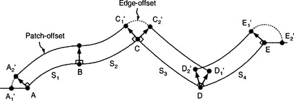
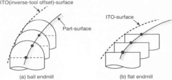
As depicted in Figure 22.12, the CL-surface is a compound surface consisting of patch-offset surfaces and edge-offset surfaces. Thus, in the offset-surface digitizing method, the CL Z-map is constructed by digitizing the individual offset surfaces. (If more than one z-value is sampled for a given grid-point, the highest is selected.) Each patch-offset surface is digitized by performing Z-map sampling on its triangulated facet-model, while edge-offset surfaces are digitized by simulating the cutting of an ‘inverse tool’, as depicted in Figure 22.13. Thus, the overall procedure for constructing the CL EZ-map (extended Z-map) may be expressed as follows:
Input: a CAD model consisting of parametric surface patches, together with the cutter geometry.
Step 1. Construct a master Z-map model using the 2D Jacobian algorithm.
Step 2. Construct a triangulated facet model for each of the patch-offset surfaces.
Step 3. Digitize each individual offset triangle in the triangulated facet-models.
Step 4. Find all the convex and boundary edges.
Step 5. Perform ‘inverse tool’ cutting simulation along each of the edges found in Step 4.
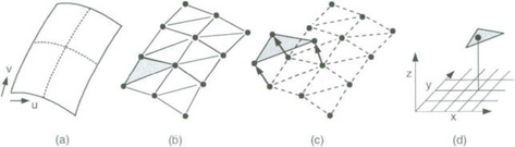
Figure 22.14-a shows a parametric surface patch whose offset surface is to be digitized. First, the surface patch is discretized and triangulated as, depicted in Figure 22.14-b, and then the vertices of each triangle are offset along their ‘offset vectors’ to obtain an offset triangle as shown in Figure 22.14-c. For a ball-endmill of radius ρ, the offset vector may be given by ρ · n, where n is the unit normal vector. Finally, as shown in Figure 22.14-d, each offset triangle is digitized.
A number of surface-discretization algorithms are available in the literature (see Austin et al. [2]). One of the key issues in discretization is the choice of an appropriate resolution, the step-length λ between two adjacent vertices, while keeping the discretization error ![]() within the input tolerance τ. A simple method is to approximate the curve joining the two vertices with a circular arc of radius ρk, so that the step length λ is givenby
within the input tolerance τ. A simple method is to approximate the curve joining the two vertices with a circular arc of radius ρk, so that the step length λ is givenby
However, as shown in Figure 22.15, the offset surface discretization error, ![]() o, is different from the base surface discretization error,
o, is different from the base surface discretization error, ![]() , although they are related to each other as follows:
, although they are related to each other as follows:
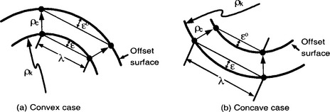
where ρc is the radius of the (ball-endmill) cutter. (The ± becomes + for a convex region and - for a concave region.) Since ![]() o ≤ τ, from the results of (22.5) and (22.6), the triangulation step-lengths λ for the convex case (Figure 22.15-a) and concave case (Figure 22.15-b) are expressed as follows:
o ≤ τ, from the results of (22.5) and (22.6), the triangulation step-lengths λ for the convex case (Figure 22.15-a) and concave case (Figure 22.15-b) are expressed as follows:
where ρk is the radius of the normal curvature in the direction of the ‘next’ vertex and ρc is the (effective) radius of the cutter (in the same direction).
It should be noted that the inequalities (22.7) and (22.8) are undefined in ‘narrow concave regions’ where the radius of normal curvature is less than or equal to the cutter radius. (Such regions are simply excluded from digitizing.)
The above procedure for determining step-length may easily be implemented for a ball-endmill. However, the procedure would be quite involved for a round-endmill because:
1. The effective cutter radius ρc is not easily computed, and
2. Inequality (22.6) is no longer valid in horizontal regions where the normal vector n of the surface is vertical. (The horizontal regions may be digitized by simulating inverse cutting.)
22.5.2 2D PS-curve offsetting
The 2D-curve offsetting problem (Tiller and Hansen [23]) has been regarded as one of the key issues in generating tool paths for 2D pocketing. In general a 2D curve may be 1) in parametric form, for instance a NURBS-curve, 2) a curve consisting of lines and arcs, or 3) a curve defined by a sequence of points (PS-curve).
The parametric-curve offsetting problem was formulated mainly in terms of self-intersectior while the main reason for offsetting a line/arc-curve was to obtain a non-self-intersecting offset curve. Line/arc-curve offset methods may further be classified into the curve-based approach and the area-based approach. The area-based methods make use of related concepts such as the bisector and Voronoi algorithms, which provide more stable means to obtain an offset curve. The subject of offsetting a PS-curve has received less attention,perhaps because it can be approximated by a line/arc-curve. However it still remains a hot issue in developing commercial SSM software.
This section describes a robust pairwise offset algorithm that obtains the valid offset curves of an input boundary PS-curve. Initially, the PS-curve is given as a closed sequence of 2D points, where each point is regarded as a vertex. In a preprocessing step, collinear vertices may be removed from the initial PS-curve. This is not essential for the algorithm but it may help speed up subsequent processes. After that, the PS-curve is converted into a counter-clockwise linked-list of segments, during which a list of pointers (to the PS-curve) for the convex vertices is also constructed. The PS-curve offsetting algorithm is described as follows (Choi [5]):
2D PS-curve offsetting
Input: PS-curve, offset direction, offset distance (ρ).
Step 1. Remove all local interfering ranges (LIR):
While (there remains a convex vertex in the PS-curve) do {
1. Get the parameter value tc of a convex vertex;
3. Perform pairwise interference detection (f, b);
step 2. Construct a raw offset curve from the remaining segments in the PS-curve.
step 3. Find all self-intersections of the raw offset curve using a sweep-line algorithm.
step 4. Remove all global interfering ranges (GIR):
While (‘unmarked’ self-intersections remain in the raw offset curve) do {
1. Select an unmarked self-intersection point P = (fs, bs) and mark it;
3. Perform pairwise interference detection (f, b);
4. Mark the self-intersection point Q = (f, b);
step 5. Construct valid offset curves from the remaining segments of the offset curve.
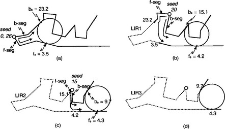
Step 1 of the algorithm will be explained with the LIR of the PS-curve that is shown in Figure 22.16. As depicted in Figure 22.16-a, the convex vertex shown as tc = 0 is selected as a local seed point in Step 1-1. In Step 1-3, the pairwise-interference-detection (PID: f, b) function is called with f = b = 0, which will return the parameter values (f = fe = 3.5, b = be = 23.2) at the contact-points of the common tangential circle. In Step 1-4, the LIR1 = [23.2, 3.5] is deleted from the PS-curve, as depicted in Figure 22.16-b. In the next iteration of the While loop, another convex vertex at tc = 20 is selected, in Step 1-1; and then, in Step 1-3, the PID function is called with f = b = 20 and the parameter values (f = fe = 4.2 and b = be = 15.1) for a new LIR are returned. Next, in Step 1–4, the new interference range, LIR2 = [15.1, 4.2], is deleted (see Figure 22.16-c). During a further iteration of the While loop, another interference range, LIR3 =[9.7, 4.3],is detected and deleted (see Figure 22.16-d). In the example shown in Figure 22.16, one may observe that a segment is visited only once, even though it may belong to more than one LIR (since LIR1 ⊂ LIR2 ⊂ LIR3).
A comment on the choice of local seed points in Step 1 may be in order. For the PS-curve of Figure 22.17, the convex vertices shown as t = 0,20, 15 (hollow points) were selected ‘at random’ as local seed points (Step 1–1 of the algorithm). In theory, the performance of Step 1 can be improved by employing an ‘optimal’ strategy for selecting a local seed point. In practice, however, defining such a strategy is not easy, and finding a better seed point imposes an additional computational burden.
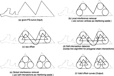
Since all the segments belonging to local interference ranges have been deleted from the PS-curve during Step 1, it now contains only five linear segments and one reflex segment (Figure 22.17-b). In Step 2 of the algorithm, a raw offset curve of the resulting PS-curve is constructed (Figure 22.17-c). In Step 3 of the algorithm, self-intersection points of the raw offset curve are computed (Figure 22.17-d).
Now we describe in detail the operations performed in Step 4 of the algorithm. In Step 4–Step 1, a self-intersection point P (Figure 22.17-d) is selected and tracing directions are assigned by setting fs = 4.5 and bs = 8.2. Since the self-intersection point P of the raw offset curve is the center point of a tangential circle of the PS-curve, the tracing directions are assigned in such a way that the tangential circle ‘gouges’ the PS-curve. Now, using the selected point P(fs = 4.5, bs = 8.2) as a global seed point, the PID (f, b) function is called with f = 4.5 and b = 8.2, in Step 4–3. The PID function will then return the parameter values at another self-intersection point Q(f = 4.7, b = 6.8). The two self-intersection points P and Q are ‘marked’ in Steps 4–1 and 4–4, respectively. In Step 4–Step 5, the global interference range, GIR = [4.5, 4.7] ∪ [6.8, 8.2], that was detected in Step 4–3 is collected.
The collected GIRs are deleted after the While loop (i.e. in Step 4–6) because otherwise small portions of some GIRs might be traced more than once.
22.5.3 Area scan algorithm
This section describes an area scan algorithm mainly used in direction-parallel area milling. The algorithm handles multiply-connected areas and is not restricted to specific types of contour elements such as line segments or circular arcs (Park and Choi [17]). For the sake of simplicity, however, we assume that the area curves are PS-curves consisting of a large number of points. In practice, area curves are usually given as PS-curves obtained from surface-surface intersections (i.e. the intersection between the CL-surface and a plane) or feature curves extracted from the CL-surface. We divide the algorithm into two modules: 1) finding the optimal inclination and 2) calculating and storing tool path elements.
Optimal inclination
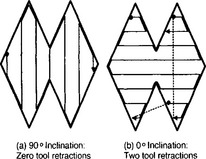
In actual machining, the inclination of milling may be decided by the user, based on technological requirements such as the feature (slope) of the part surface or constraints imposed by the machining configuration (NC-machine, jigs and fixtures). Otherwise the tool path planning system should be able to find an optimal inclination that satisfies three objectives: 1) minimizing the number of tool retractions, 2) minimizing the number of toolpath elements and 3) maximizing the average length of tool path elements. Figure 22.18 shows that the inclination is related to three objectives.
Note that the number of tool retractions may not be decided by the inclination alone, because it is also influenced by the tool path linking method. In order to incur the minimum number of tool retractions, some researchers have suggested algorithms that perform two-step optimizations: global optimization (selecting optimal inclination) and local optimization (tool path linking method). But for the other two objectives, minimizing the number of tool path elements and maximizing the average length of tool path elements, there is no available prior research, to the best of our knowledge. We do not explicitly consider the average length of tool path elements, because the minimum number of tool path elements will in any case maximize their average length.
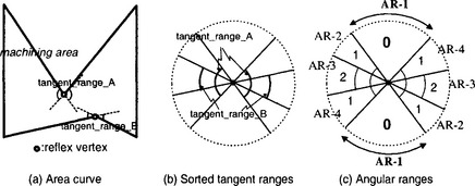
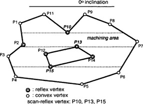
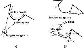
Before giving a formal description of the proposed module, we first introduce some basic terminology. A vertex is called reflex if the internal angle between its incident segments is greater than π, and convex otherwise (Figure 22.19). Given some inclination, a reflex vertex v is called a scan-reflex vertex if there is a neighborhood δ at v such that the boundary of the inside area is on one side of the line parallel to the inclination and passing though v (Figure 22.19). A sequence of consecutive reflex vertices is called a reflex profile if its tangent range is smaller than π (Figure 22.20-a), otherwise it is divided into several reflex profiles (Figure 22.20-b). Note that a reflex profile has at most one scan-reflex vertex with respect to an arbitrary inclination. The length of a reflex profile is defined as the sum of the lengths of all its segments.
To fulfil the objectives listed above, an inclination should be chosen by considering not only the geometric shape of the area but also the tool path interval. Some researchers have suggested algorithms that select an inclination which minimizes the number of local extrema (scan-reflex vertices), but without considering the tool path interval. As a result these algorithms may not properly deal with the local (small) features of the boundary curves and thus fail to minimize the number of tool path elements.
The proposed module has to find the inclination that minimizes the number of scan-reflex vertices after removing reflex profiles with a length smaller than the tool pathinterval, and also local (small) features. The algorithm is described as follows:
Step 1. Identify all the reflex vertices on the area curve, and construct a reflex profile set by grouping consecutive reflex vertices.
Step 2. Remove reflex profiles with a length smaller than the tool path interval from the reflex profile set. (Local features are removed from the reflex profile set.)
Step 3. Compute tangent ranges of the reflex profiles in the set and sort them (Figure 22.21-b).
Step 4. Find an angular range belonging to the smallest number of tangent ranges (Figure 22.21-c).
Step 5. Pick the central inclination inside the selected angular range.
Note that the angular range found in Step 4 contains the minimum number of scan-reflex vertices because a reflex profile gives at most one scan-reflex vertex when the inclination belongs to the tangent range
Calculating and storing tool path elements
This module has two objectives: one is to find tool path elements efficiently and the other is to store them in a suitable data structure for tool path linking. For the former purpose, we use the plane sweep paradigm and the concept of a monotone chain. A graph-like structure, the tool path element net (TPE-net) is suggested to achieve the latter goal.
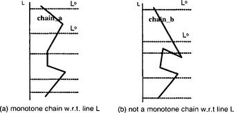
A chain C is monotone with respect to a line L if C has at most one intersection point with each line L° perpendicular to L (Figure 22.22-a). The line L is called the monotone direction and the line L° becomes a sweep line.
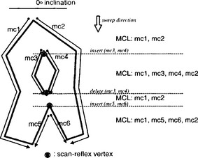
Without loss of generality, we may assume that the x-axis (0°) is the inclination found in the previous module: i.e. the reference lines (or tool path elements) are horizontal. Firstly, we decompose area curves into monotone chains with respect to the y-axis. After decomposition, the tool path elements are calculated by sweeping a horizontal line across the monotone chains from top to bottom. During sweeping we maintain a monotone chainlist (MCL) which is crossed by a reference line, and the list is ordered by the x-values at their intersection. Note that the number of monotone chains is not changed unless the sweep passes over a scan-reflex vertex. At an event corresponding to a scan-reflex vertex v, a pair of monotone chains is inserted into the MCL if v has a local maximum y-value, or deleted from the MCL if v is locally minimal (Figure 22.23). Then at each reference line, the tool path elements can easily be obtained by checking intersections between the reference line and the monotone chains in the MCL.
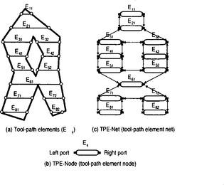
A tool path element Eij is intuitively represented using the ‘TPE-node’ (tool path element node) (Figure 22.24-b). We suggest a graph-like structure to denote the connectivity relationships among TPE-nodes called a TPE-net (tool path element net) consisting of TPE-nodes and arcs (Figure 22.24-c). Note that to achieve the fifth requirement ‘movement along boundary curves’, every arc in the TPE-net should contain geometric information about the corresponding segment of the boundary curve. Owing to the intuitiveness of the TPE-net, we can easily construct and handle it in the next module, tool path linking.
22.5.4 Point-sequence curve fairing
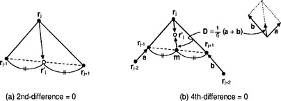
This section describes a fairing algorithm for a PS-curve such as a pencil curve consisting of pencil-points. In this case, the 3D coordinates rj = (xj, yj, zj) of points can be decomposed into ‘domain’ coordinates pj = (xj,yj) and ‘height’ coordinates qj = (sj, zj), where sj is the cumulative length of the PS-curve given by
PS-curve fairing is performed using a systematic fairing scheme based on difference operators. Our strategy is to apply the point-data fairing operations separately to the domain coordinates (pj) and the height coordinates (qj).
For a 3D point sequence rj, the n th difference is defined as
Then, by setting Equation (22.10) to zero for n = 2, the ‘ideal’ position ![]() for the input point rj can be computed from the 2nd-difference fairing equation given by
for the input point rj can be computed from the 2nd-difference fairing equation given by
Similarly, by setting Equation (22.10) to zero for n = 4, the ideal position ![]() can be computed from the 4th-difference fairing equation given by
can be computed from the 4th-difference fairing equation given by
The physical meaning of the above fairing equations is shown in Figure 22.25: 2nd-difference fairing straightens the curve, while 4th-difference fairing leads to a curve withlinear change in curvature (if the point spacing is uniform). In the literature, a quantity similar to the sum of squares of the right-hand side terms in Equation (22.12) is often used as a global smoothness measure of a digitized curve (Eck and Jaspert [11]). For local straightening, we use the 2nd-difference fairing equation (22.11), while the 4th-difference fairing equation (22.12) is employed for global smoothing.
In practice, the input point sequence may have uneven spacing. Thus, the above fairing expressions have to be normalized with respect to their chord lengths. For this purpose, we will define the following quantities:
Then, from Equations (22.11) and (22.12), the following ‘normalized’ fairing equations may be obtained:
and
where d0 = (d−1 + d+1)/2. Note that Equations (22.14) and (22.15) become equivalent to Equations (22.11) and (22.12) when we have d−2 = d−1 = d+1 = d+2
In actual fairing, the ‘faired’ position ![]() is usually determined by taking a linear combination of the ideal position
is usually determined by taking a linear combination of the ideal position ![]() and the input point rj, as follows:
and the input point rj, as follows:
where φ ∈ [0,1] is a damping factor and φ is a fairing tolerance. The blending operation (22.16) is often called a ‘damping correction’. In practice, a damping factor of 0.4 to 0.6 is commonly used.
Domain-coordinates fairing
To fair the domain-coordinate points {pj}, the ideal position ![]() can be obtained by applying the normalized fairing equations in (22.14) and (22.15). Thus, we have:
can be obtained by applying the normalized fairing equations in (22.14) and (22.15). Thus, we have:
and
where d0 = (d-1 + d+1)/2 and {di } are defined as follows:
The 2nd-difference fairing equation (22.17) is used for local straightening of the domain coordinates of the pencil-points, and the 4th-difference fairing (22.18) is used for global smoothing. In Equations (22.17) and (22.18), the damping-correction operation (22.16) is applied to the ideal position p′j and the input-point pj in order to obtain a corrected position p″j. That yields:
where φd and τd are the damping factor and fairing tolerance for the domain fairing.
Height-coordinates fairing
A unique feature of the process of fairing the height coordinates is that 1) only height values {Zj} in {qj = (sj, zj)} are allowed to move and 2) the domain chord-lengths {Sj} are used in normalizing the fairing expressions. We define the following quantities:
Then, from Equations (22.14) and (22.15), we obtain the normalized fairing expressions for {qj = (Sj, Zj)} given below:
and
where d0 = (d−1 + d+1)/2.
The ‘faired’ position ![]() is obtained from the following correction operation:
is obtained from the following correction operation:
where φh is the damping factor and τh is the fairing tolerance for the height-fairing.
Overall fairing procedure
Based on the results presented so far, the overall PS-curve fairing procedure may be summarized as follows:
Step 1. Local ‘saw-tooth pattern’ straightening of {pj} by employing Equations (22.17) and (22.19).
Step 2. Global smoothing of {pj} using Equations (22.18) and (22.19).
Step 3. Local ‘saw-tooth pattern’ straightening of {Zj} utilizing Equations (22.20) and (22.22).
Step 4. Global smoothing of {Zj} using Equations (22.21) and (22.22).
At each step, the correction operation from Equation (22.19) or (22.22) is applied repeatedly. In each iteration, only the data points that have a ‘local maximum’ deviation are corrected, and the iteration is terminated when no significant improvement is observed.
For this purpose, we define the deviation vj of a data point (from the ideal position) to be
Then, in a local straightening, the j-th data point may be corrected only when vj > max(vj−1, vj+1) is satisfied. In a global smoothing, the j-th data point is corrected when we have vj > max(vj−2, vj−1, vj+1, vj+2).
22.5.5 Collision detection algorithms
In the C-space approach described in Section 22.4.1.2, ‘rapid-move’ collisions can be avoided by preventing rapid-moves (G00 NC code blocks) from entering the machining C-space volume VM. This is equivalent to confining the rapid moves to the space above the preform CL-surface Sp.
The C-space method allows a straightforward mechanism for preventing collisions during cutting moves (G01 or G02/03 NC code blocks) as well. As shown in Figure 22.26-a, an endmill assembly consists of four elements: cutting-edge, dead-center, shank and holder. Cutting actions take place only at the cutting edge. The dead-center is the center region of the base of the endmill, which has no cutting capability. If a non-cutting element is in contact with the workpiece during a machining operation, a ‘cutting-move’ collision occurs. Thus, there are three types of cutting-move collision: dead-center collision, shank-collision and holder-collision.
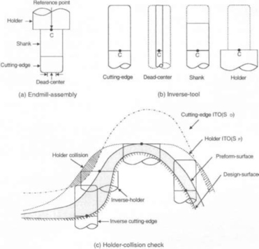
It should be observed that a dead-center collision can only occur during downward milling, while a shank collision may occur during upward milling. On the other hand, a holder collision can occur in both downward and upward milling. Now, as depicted in Figure 22.26-b, we define an ‘inverse’ tool (IT) for each element of the endmill-assembly: a cutting-edge IT, a dead-center IT, a shank IT and a holder IT. Note that we use the same reference point C in all the inverse tools. The next step is to generate ITO (inverse tool offset) surfaces as follows:
1. The cutting-edge ITO surface is the design CL-surface (SD) for the cutting-edge IT.
2. The dead-center ITO surface is the preform CL-surface (Sp) for the dead-center IT.
3. The shank ITO surface is the preform CL-surface (Sp) for the shank IT.
4. The holder ITO surface is the preform CL-surface (Sp) for the holder IT.
Then a necessary condition for a holder collision is that “there exists a region where the holder ITO surface is higher than the cutting-edge ITO surface”, as indicated in Figure 22.26-c. Similarly, a necessary condition for a shank collision (dead-center collision) may be expressed as “there exists a region where the shank ITO surface (dead-center ITO surface) is higher than the cutting-edge ITO surface when the endmill is moving upward (downward)”.
The C-space-based collision-detection procedure introduced in this section is not limited to roughing. It is applicable to any type of 3-axis NC machining.
22.6 CONCLUSION
Sculptured surface machining (SSM) is a means to realize sculptured surfaces created by engineering designers and often becomes a vital part of other non-machining processes,such as sheet-metal stamping and plastic injection molding. CAGD people should know about the SSM process because 1) geometric problems of SSM are closely related to CAGD and 2) the seamless connection of product design and the SSM process is a key factor in improving product quality while reducing development time.
This chapter has introduced the SSM (sculptured surface machining) process, including the UMO (unit machining operation) and identified the geometric issues that occurr in the information processing stages of SSM, which are as follows: 1) interference handling, 2) CL-surface construction for the C-space approach, 3) 2D PS(point sequence)-curve offsetting, 4) area scan algorithms, 5) PS-curve fairing and 6) collision detection algorithms.
1. Altan, T., et al. Advanced techniques for die and mold manufacturing. Annals of the CIRP. 1993;42(2):707–716.
2. Austin, S., Jerard, R.B., Drysdale, S. Comparison of discretization algorithms for NURBS surfaces with application to numerically controlled machining. Computer-Aided Design. 1997;29(1):71–83.
3. Choi, B.K., et al. Triangulation of acattered data in 3D space. Computer-Aided Design. 1988;20(5):239–247.
4. Choi, B.K., Jun, C.S. Ball-end cutter interference avoidance in NC machining of sculptured surfaces. Computer-Aided Design. 1989;21(6):371–378.
5. Choi, B.K. Surface Modeling for CAD/CAM. Elsevier; 1991.
6. Choi, B.K., et al. Development of a 9-axis marine propeller machining system. Final Report submitted to Hyundai Heavy Industries Ltd, KAIST, Korea (in Korean). 1991.
7. Choi, B.K., Kim, D.H., Jerard, R.B. C-space approach to tool-path generation for die and mold machining. Computer-Aided Design. 1997;29(9):657–669.
8. Choi, B.K., Park, S.C. A pair-wise offset algorithm for 2D point-sequence curve. Computer-Aided Design. 1998;31(12):735–745.
9. Choi, B.K., Jerard, R.B. Sculptured Surface Machining. Amsterdam: Kluwer Academic Publishers; 1998.
10. Duncan, J.P., Mair, S.G. Sculptured Surfaces in Engineering and Medicine. Cambridge University Press; 1983.
11. Eck, M., Jaspert, R. Automatic fairing of point sets. In: Sapidis N., ed. Designing Fair Curves and Surfaces. Cambridge - London - New York: SIAM; 1994:44–60.
12. Fallbohmer, P., et al, Survey of the U.S die and mold manufacturing industry. ERC/NSM-D-95-41. The Ohio State University, 1995.
13. PED 59 Jensen, C.G., Anderson, D.C., Accurate tool placement and orientation for finish surface machining. Concurrent Engineering. ASME: U.S.A., 1992:127–145.
14. Marshall, S., Griffiths, J.G. A new cutter-path topology for milling machines. Computer-Aided Design. 1994;26(3):204–214.
15. Mason, F. 55 for high-productivity airfoil milling. American Machinist. 1991:37–39.
16. Murray, R.M., et al. A Mathmatical Introduction to Robotic Manipulation. CRC Press; 1994.
17. Park, S.C., Choi, B.K. Tool-path planning for direction-parallel area milling. Computer-Aided Design. 2000;32(1):17–25.
18. July Saito, T., Takaashi, T. NC Machining with G-buffer method. Computer Graphics. 1991;25(4):207–216.
19. Schulz, H., Hock, S. High-speed milling of dies and moulds – cutting conditions and technology. Annals of CIRP. 1995;44(1):35–38.
20. Sheng, X., Hirsch, B.E. Triangulation of trimmed surfaces in parametric space. Computer-Aided Design. 1992;24(8):437–444.
21. Suresh, D.J., Yang, D.C.H. Constant scallop height machining of free form surfaces. Journal of Engineering for Industry. 1994;116:253–259.
22. (in Japanese) Takeuchi, Y., et al. 5-axis control machining based on solid model. J. Precision Eng. 1990;56(11):111–116.
23. September Tiller, W., Hansen, E.G. Offset of two-dimensional profiles. IEEE Computer Graphics and Applications. 1984;4(9):36–46.