Cyclides
23.1 INTRODUCTION
Cyclides were detected and first studied by Ch. Dupin (1784-1873) in [22] and are since called “Dupin cyclides”. At that time differential geometry was in a very early stage: Only some investigations of L. Euler (1707-1783) and the fundamental work of G. Monge (1746-1818) “L′Application de l′analyse à la géométrie” proceeded but the famous treatise of C.F. Gauss (1777-1855) “Disquisitiones generales circa superficies curvas” appeared only a few years later.
In parallel, after projective geometry was founded by Poncelet (1788-1867), research on algebraic curves and surfaces had a first blossom. Dupin cyclides belong to both of these areas: In differential geometry, they can be defined as surfaces having constant main curvatures along the corresponding curvature lines. This property has been widely generalized into the differential geometry of manifolds in higher dimensional spaces up to present (see [13] for instance).
On the other hand, they are algebraic surfaces of fourth or third order 1being simultaneously enveloped by two families of spheres. This latter property is characteristic and serves often as an alternative definition. As algebraic surfaces they can be represented by a single polynomial equation of degree up to four; but they proved, in addition, to be rational, thus they can be parametrized by quadratic functions of u and v. These two kinds of representations that can be converted into each other confers the Dupin cyclides many advantages, in particular with respect to applications.
It was soon realized that Dupin cyclides of fourth order have the isotropic circle at infinity as its double curve. This gave rise to extensive investigations on algebraic surfaces. Kummer [29] and Casey [11] found interesting generalizations of Dupin cyclides, 2howeverthese topics must be renounced in the present chapter (see the excellent treatise of Jessop [25] for details).
But there is another intermediate class of surfaces, found by Degen [15–17], they are defined to be the envelope of two families of general quadrics such that each of these quadrics is tangent to the surface along a conic, with the additional property that these conics build up a conjugate net on the surface (what holds also for Dupin cyclides). These surfaces, now called “supercyclides” (originally “double Blutel surfaces”) will be treated in section 23.3.
Dupin cyclides were recovered for CAGD purposes about 1988; they extended the class of surfaces so far used in geometric modeling (essentially the natural quadrics) considerably. In particular, the virtues of cyclides were realized when serving as blending surfaces. Still much more flexibility is attained by using supercyclides. The long list of papers that since appeared show the importance of cyclides and supercyclides in CAGD.
23.2 THE GEOMETRY OF DUPIN CYCLIDES
23.2.1 Dupin cyclides in classical differential geometry
As usual in local differential geometry, one starts with a regular surface patch in parameter representation φ … x: I1× I2→ IR3. where the curvature lines are used as iso-parameter lines. (This is possible if the patch has no umbilics; see [10] for basic information on classical differential geometry). They will be denoted by C1(v0) = {x(u, v0) | u ∈ I1} and C2(u0) = {X(u0, v) | v ∈ I2}. We further assume differentiability (at least x∈ C3[I1× I2]) and regularity xu ∧xv ≠ 0 throughout.
Let n: I1× I2→ IR3 be the normal vector field (n = xu ∧ xv/ ![]() xu∧xv
xu∧xv ![]() ), then the formulas of Rodrigues and the defining property of the Dupin cyclides are expressed by 3
), then the formulas of Rodrigues and the defining property of the Dupin cyclides are expressed by 3
This implies that the curvature centers
depend only on one parameter, thus describing two curves P… p: I1→ IR3, Q… q: I2→ IR3. Furthermore we consider the curvature spheresS1(u) (S2(v)) having p(u) (q(v)) as mid point and r2(u) (respectively r1(v)) as radius 4and conclude that they also depend only on one parameter. Obviously, the curvature spheres S1(v) and S2(u) touch each other at the surface point x(u, v); but by n˜p- qboth are tangent also to Φ at that point. Thus both families of curvature spheres envelope the cyclide; if one of them moves through its family and another one of the other family is kept fixed, the points of contact generate the corresponding curvature line. But since the characteristics(defined as ![]() ) of a one parameter family of spheres are circles, so are the curvature lines of a Dupin cyclide. Furthermore, as [p(u), p′(u)] is the rotational axis ofthe enveloping cone C*2(u0) its apex a(u0) does not depend on v and thus all the planes of C1(v) (v ∈ I1) contain the tangent a1:= [a(u), a′(u)]. Since these planes do not depend on u, this line a1is fixed in space. Hence these planes belong to a pencil with axis a1. As the analogous properties hold also for the other family, we can summarize:
) of a one parameter family of spheres are circles, so are the curvature lines of a Dupin cyclide. Furthermore, as [p(u), p′(u)] is the rotational axis ofthe enveloping cone C*2(u0) its apex a(u0) does not depend on v and thus all the planes of C1(v) (v ∈ I1) contain the tangent a1:= [a(u), a′(u)]. Since these planes do not depend on u, this line a1is fixed in space. Hence these planes belong to a pencil with axis a1. As the analogous properties hold also for the other family, we can summarize:
Theorem 1
(a) The focal surfaces of the normals of a Dupin cyclide5degenerate into two curvesPandQ. (b) The curvature spheres of a Dupin cyclide consist of two one parameter families S1and S1. (c) Each curvature sphere envelopes the cyclide along a curvature line (more preciselyS2(v0) is tangent to Φ along the curvature lineC1(v0) and, analogously, S1(u0) is so alongC2(u0)). (d) All the curvature lines are circles. 6Their planes belong to two pencils (more precisely: the planes ofC1(v0) belong to the pencil with axis a1, those ofC2(u0) belong that one with axis a2. (e) The apexesa(u) of the circumscribed cones alongC2(u) lie on the axis a1and those of the other family, b(u), lie on a2. (f) The mid point curvesPandQare planar curves whose planesEandFcontain the axes a1and a2respectively.
The last property (f) is implied by the fact that the tangent [p(u), p′(u)] meets the axis a1and analogously for the other family. — Finally, simple geometric reasoning leads to
Theorem 2
(a) The mid point curvesPandQof the two families of enveloping spheres are conics lying in two planesEandFwhich are orthogonal to each other and symmetry planes of the cyclide. (b) both axes a1and a2are orthogonal to the intersection line1:= E∪ F. (c) One of the curvesPorQ, sayQ, may degenerate into a straight line; thenQmust coincide with a2and a1is inEat infinity.
Furthermore, from (23.2) one can take
Thus the surface is determined once the curves Pand Qas well as the radius functions r1and r2are known.
As the radius functions can be replaced by ![]() (while the normals are maintained) one gets:
(while the normals are maintained) one gets:
Theorem 3
The offset surfaces of a Dupin cyclide are again Dupin cyclides; they share the same normals with the original cyclide and have the radius functions with an arbitrary constant c added7.
It remains to determine the exact possibilities of the different kinds of conics that can be combined to a pair of curves Pand Qfor a Dupin cyclide. This will be done in the next section.
23.2.2 The three main types of Dupin cyclides and their parameter representations
There are the following three types of regular Dupin cyclides
I Tori:Pis a circle, the surface is rotationally symmetric, Qdegenerates into a line being simultaneously the second axis a2and the axis of rotation. The first axis a1is in the planeEat infinity.
II General Dupin cyclides:Pis an ellipse inEandQisa hyperbola inF, orthogonal toE. These conics share their vertices and foci but with reversed roles. All these points lie on1 = E∩ F. The axes a1and a2lie inE, Frespectively and are orthogonal to1.
III Parabolic Dupin cyclides:P and Q are both parabolas having1as their common axis. They also share their vertex and focus in reversed roles.
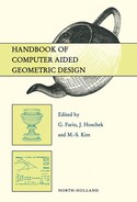
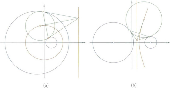
Proof: The exceptional case of a torus is already contained in Theorem 3. In all the other cases, P and Q are true real conics. Since E and F are symmetry planes, the vertices lie on 1. In the plane E there are the intersection circles D1(u) = S1(u) ∪ E of the first family of spheres S1, having their mid points at p(u). From the other family S2there is at least one profile circle D2(v0) having its mid point at (one of) the vertex q(v0) on 1. Thus, all the circles D1(u) touchD2(v0) at X(u, v0). Furthermore, thetangents to P at p(u) and to D2(v0) at x(u, v0) ⊂E must intersect on the point a(u) of a1.
Figure 23.2 The two enveloping spheres at a point of a Dupin cyclide and the mid point curves in the symmetry planes.
These conditions can be exploited with methods of elementary geometry in all the three cases when P is an ellipse, a hyperbola or a parabola. The crucial conclusion is the following: Using a rational parametrization in any case, setting a(u) = (d, α(u), 0) in a suitable coordinate system with 1 as x-axis, E as x-y-plane and F as x-z-plane one gets for α a rational function. This implies that ![]() must be rational too. The radicand of ω(u) turns out to be a biquadratic function and so it must be a complete square. The calculations with coordinates yield in any case that q(v0) is a focal point of P.
must be rational too. The radicand of ω(u) turns out to be a biquadratic function and so it must be a complete square. The calculations with coordinates yield in any case that q(v0) is a focal point of P.
Elaborating this idea yields for Q a hyperbola when P is an ellipse, an ellipse when P is a hyperbola and a parabola when P is a parabola. Since in the first two cases only the two curves P and Q are permuted, there remain, besides the tori, only the two further cases of the theorem.
The parameter representations of the Dupin cyclides are obtained by (23.3). We use rational parameters for P and Q in all cases (They can, if wanted, easily be convertedinto trigonometric forms by setting ![]() and
and ![]() and likewise for v.) Then the radius functions are obtained by the method described above. One obtains the following results:
and likewise for v.) Then the radius functions are obtained by the method described above. One obtains the following results:
Case I. Tori:
Parameter representation of the cyclide:
Depending on the ratio of R and r, there are three subcases of tori:
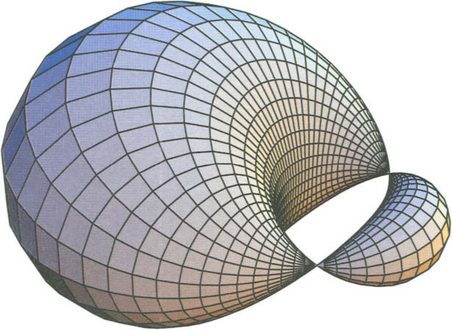
1. r > R: All the spheres S1(u) intersect the second axis a2in a pair real, different points where the radius function r1has zeros and the cyclide has singular points (like the apex of a cone); it is called a “spindle cyclide”.
2. r = R : The axis a1is is tangent to all the spheres S1(u) of S1. The surface has a singularity (a sharp double spike) at the point of contact and is called “limit torus”.
3. r < R: The spheres S1(u) don′t intersect. The surface has no singularities and is ring-shaped.
Case II. General Dupin cyclides
with f2 = a2- b2 saying that q(v0) is a focal point 8of P.
Parameter representation of the cyclide:
From these formulas one can take that there are three subcases for each of the positions of the axes with respect to P and Q respectively. However, since both axes depend on the same parameter c there are only the following five subcases:
1. c < f: The axis a1intersectsP in a pair of real, different points where the radius function r2has zeros and the cyclide has singular points (like the apex of a cone); it is called a “spindle cyclide”.
2. c = f: The axis a1is is tangent to P at the point (a, 0, 0) and so are all the spheres of S1. The surface has a singularity (a sharp double spike) at that point.
3. f < c < a: Both axes don′t intersect P or Q. The surface has no singularities and is ring-shaped. The second axis a2passes through the hole while the first one lies outside the surface.
4. c = a: The axis a2is is tangent to Q at the point (f, 0,0) and so are all the spheres of S2. The surface has a singularity (a sharp double spike) at that point.
5. c > a: The axis a2intersectsQ in a pair of real, different points where the radius function r1has zeros and the cyclide has singular points (like the apex of a cone); it is called a “horn cyclide”.
Case III. Parabolic Dupin cyclides
(where the mid point between the vertex and focus serves as origin).
with an arbitrary constant c. One can assume c ≥ 0 since otherwise the two parabolas can be permuted.
Theorem 5
Parabolic Dupin cyclides contain both their axes as degenerated curvature linesC1(∞) andC2(∞) respectively.
This is an essential difference to both the other main classes: In general, a certain plane of a curvature circle intersects the cyclide of class I or II yet in another curvature circle (of the same family) in accordance with the fact that it is an algebraic surface of fourth order (see section 23.2.3). But if the cyclide is parabolic, then the intersection of a plane from the pencils through the axes, the intersection consists of the axis itself and the corresponding curvature circle in accordance with the fact that parabolic cyclides are of the third order.
23.2.3 Implicit equations
By eliminating the parameters in the representations (23.6), (23.9), (23.15), one gets the following implicit representations of the corresponding cyclides.
Case I. Tori:
So the tori are algebraic surfaces of fourth order. The terms of fourth order being (x2 + y2 + z2)2 confirms that the isotropic circle at infinity is the double curve of ΦI.
Case II. General Dupin cyclides
The implicit equation of general Dupin cyclides is:
So the general Dupin cyclides are, like the tori, algebraic surfaces of fourth order. The terms of fourth order are the same as for tori; this confirms that the isotropic circle at infinity is the double curve also for the general Dupin cyclides.
One can see that this equation carries over to (23.16) for f = 0 and with R = a, r = c. So a torus can be considered as a limit case of a general Dupin cyclide (the abscissa of a1tends to ∞ and that of a2to 0 in accordance with Theorem 4, I).
Case III. Parabolic Dupin cyclides
For parabolic Dupin cyclides parameter elimination yields
So the parabolic Dupin cyclides are algebraic surfaces of third order and the intersection with the plane at infinity splits into the isotropic circle and the straight line x = 0.
One realizes that the two axes a1… x = −c − f, z = 0 and a2… x = − c + f, y = 0 are contained in ΦIII. So the planes of the two pencils with those axes intersect the surface in that axis and one of the generating circles C1(v) respectively C2(u).
23.3 SUPERCYCLIDES
23.3.1 Curves and surfaces in the projective space
In this Section we use projective geometry throughout. This has many advantages in theory as well as in applications: There is no need to distinguish between intersecting and parallel lines and planes, or between cones and cylinders and all rational parametrizations can be converted into polynomial ones simply by a renormalization. (For basic information see [8], Ch. V). In particular, points are represented by vectors p ∈ IR4 {(0, 0, 0, 0)} that can arbitrarily renormalized by ![]() = ρp with ρ ∈ IR {0}.
= ρp with ρ ∈ IR {0}.
Curves and surfaces are represented by vector-valued differentiable functionsx: D → IR4 where D is an real interval for curves and an open, connected domain of IR2 for surfaces. In both cases, the representation can be renormalized (without changing the geometric object) by an arbitrary real-valued differentiable function ρ :D → IR {0}.
23.3.2 Basic properties of supercyclides
Now we turn to supercyclides. However we must renounce all the theoretical results leading to the properties and the representation we will describe in the sequel (see [15]–[17] and [5] for the details). Furthermore, there is a slight difference between the notions of a “double Blutel surface” and a “supercyclide”. However, in order to allow a unifiedtreatment, we exclude supercyclides with intersecting axes (see Theorem 6) but include those of third order (as in the case of Dupin cyclides); nevertheless we maintain the term “supercyclide” for shortness.
Furthermore we emphasize that Dupin cyclides are special supercyclides with additional properties coming from the Euclidean structure of the space. So supercyclides share many properties with Dupin cyclides and it turned out that, indeed, most of them are complex projective transforms of Dupin cyclides [5].
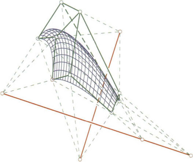
The theory leads to the final result that the supercyclides (in the sense described above) have a common parameter representation of the following type
where p(u) and q(v) are defined by
Furthermore, a, b are base points for the first axis a1and c, d are base points for the second axis a2(all the four vectors together build a basis of IR4 since the axes are assumed to be skew). In addition, it is assumed that A, B, F(C, D, G) are linearly independent quadratic functions of u(respectively of v).
Surfaces with a representation of the form (23.19) are called projective translation surface(see [20], compare with (23.3)). Furthermore, renormalizing with F yields
and a similar equation is obtained by renormalizing with G(v). This shows:
Theorem 6
(a) The iso-parameter linesC1(v0) : v = v0andC2(u0) : V = v0are non-degenerated conics, (b) The planesE1(v0) of C1(v0) contain the first axis a1(so belonging to a pencil), (c) The planesE2(u0) ofC2(u0) contain the second axis a2(so belonging to a pencil).
Since the parameter λ = D (v)/C(v) controls the position of E1(v) within the pencil (or the point q(v) on the second axis a2), we conclude: Every planeEλof the pencil through a1intersects the surface in a pair of conicsC1(v1), C1(u2) where v1, v2are the roots of the equation λC(v) - D(v) = 0 (possibly being complex or coincident). This property suggests that the surface has order four.
However the two quadratic functions may have a common root: Then the corresponding linear factor cancels at the quotient for λ, so the mapping v → λ = D(v)/C(v) is fractal linear, hence bijective from ![]() onto itself 9; furthermore, observing (23.19), one realizes that in this case all the conics C2(u) pass through the intersection point p(u) of E2(u) with the first axis a1, i.e. this line is completely contained in the surface.
onto itself 9; furthermore, observing (23.19), one realizes that in this case all the conics C2(u) pass through the intersection point p(u) of E2(u) with the first axis a1, i.e. this line is completely contained in the surface.
Of course, the same considerations can be applied to the second family of conics and their planes. So one has to distinguish between the following three classes of supercyclides:
I General supercylides: None of the pairs A, B and C, D of quadratic functions has a common root.
II Semi-parabolic supercylides:C, D have a common root, but not A, B.
III Parabolic supercylides: Both of the pairs A, B and C, D of quadratic functions have a common root.
The semi-parabolic supercyclides have almost been neglected in the literature (only mentioned in [16] and [42]). So we do not draw the reader’s attention to that case in the sequel. A second reason for this is that all the Dupin cyclides are contained in the Classes I and III, but not in Class II. (The tori and the general Dupin cyclides in Class I; the parabolic Dupin cyclides in Class III.)
Theorem 7
Supercyclides of the Classes I, II are algebraic surfaces of the fourth order, those of the Class III are of third order.
Besides the possession of two families of conics, the supercyclides (of all the three classes) have the dual property: They are enveloped by two families of quadratic cones ![]() and
and ![]() in such a way that the tangents to the conics C1(v) (v varying) along the points of a fixed conic C2(u0) coincide with the generators of the cone
in such a way that the tangents to the conics C1(v) (v varying) along the points of a fixed conic C2(u0) coincide with the generators of the cone ![]() . (This means that the tangent planes of the surface, taken along the conic C2(u0), envelope the cone
. (This means that the tangent planes of the surface, taken along the conic C2(u0), envelope the cone ![]() .) The same property holds for the permuted families of conics and cones.
.) The same property holds for the permuted families of conics and cones.
This can easily be seen by differentiating (23.19) with respect to u say:
with A* = A′ F − A F′, B* = B′ F − B F′(note that these functions are also quadratic). So the point on the right hand side of (23.23)does not depend on v and represents the apex of C*2(u)0. So one realizes that the apexes of the enveloping conesC*2(u) andC*1(v) lie on the first and second axis respectively.(Thus the axes are self-dual, since the apex of a cone corresponds to the plane of a conic by duality.)
Equation (23.19) contains even more information: Looking into one fixed plane, say E1(v0), one can see therein three objects: 1) the conic C1(v0), 2) the first axis a1and 3) the intersection point q(v0) of E1(v0) with a2. Since their coefficients do not depend on v all these configurations are protectively equivalent to each other and the same is true for the other planes E2(u0). More precisely, for any pair of planes E1(v1) and E1(v2), these configurations can even be projected onto each other from a third point on the second axis: One takes from (23.19) x(u, v2) = p(u) + q(v2) = x(u, v1) + z with z = (q(v2) - q(v1) and this proves the assertion, z being the projection center.
The different positions of these objects to each other lead to the further classification of supercyclides. In particular, the first (second) axis a1(a2) can intersect the conic C1(v0) (C2(u0)) in two different real points leading to two simple singular points on that axis orit can be tangent to it leading to a higher singularity, a sharp double spine. (Note that in both cases these intersection points do not depend on v0(u0resp.)).
Omitting the further details (to be found in [16]), we mention only, that the polarity of q(v0) and a1has the geometric meaning that the cyclide is a projective canal surface(see [9]) and if this holds for both families then it is a quadric. On the other hand, supercyclides of Class I have the following normal form(23.19), (23.20):
Furthermore, one of the coefficients σ0, σ2(T0, T2resp.) can be normalized to one if it does not vanish. So there remain two invariants(to be interpreted as cross ratios) κ1 = σ0σ2 and κ2 = T0T2determining the supercyclide:
Theorem 8
A supercyclide of Class I can be transformed into the normal form(23.24) and is determined by the two projective invariants κ1, κ2up to a projetivity of space.
23.4 CYCLIDES IN CAGD
23.4.1 Bézier representation of cyclides
As being rational biquadratic surfaces, cyclides can be represented in Bézier form and thus integrated into CAD systems. In section 23.2, we used the basis functions T0(u) = 1 + u2, T1(u) = 1 - u2, T2(u) = 2u which are linearly independent. So they can be converted into the Bernstein basis functions B0(u), B1(u), B2(u) by the matrix
Applying this to (23.9) for instance immediately yields the Bézier form in homogeneous coordinates. The component x0of x(u, v) is the denominator of the usual Euclidean vector and the coefficients at the Bernstein polynomials are its weights. This can be done by any computer algebra system.
However this would be a very special patch on that Dupin cyclide. To attain the whole flexibility, i.e. an arbitrary patch on it, one has to perform a parameter transformation
first, so that the desired boundary curves belong to parameter values ū= 0 and ū= 1 and similarly with v.
A second method consists of constructing the cyclide directly by starting with its boundary curves (circular arcs in the case of Dupin cyclides) and then observing its general geometric properties derived in the previous sections. When doing this, there arise two questions: a) What are the conditions on the control points and weights of a second order rational Bézier curve to be a circular arc? - b) What is a complete set of conditions characterizing a (Dupin) cyclide?
As to question a), given the Bézier representation ![]() one defines
one defines ![]() and v2so that v1;v2are a ON basis, then the conditions for a circular arc are
and v2so that v1;v2are a ON basis, then the conditions for a circular arc are
The second question is more complicated. In the case of a Dupin cyclide, It can be split into two steps: Take first the conditions being sufficient for a supercyclide (since any Dupin cyclide is a special supercyclide) and then add the conditions which characterize the Dupin cyclides among the supercyclides. As to the first step, these conditions were given in [17]; they can be derived by the same method described above, but now applied to (23.19): Expanding the polynomials A, B, C, … into the Bernstein basis, say ![]() etc. one obtains by inserting this into (23.19)
etc. one obtains by inserting this into (23.19)
(σi, Tk being the coefficients of F and G respectively). The resulting representation in homogeneous coordinates can be converted into a Euclidean one as before.
The following result [21], which is quoted without proof gives the answer to the second step:
23.4.2 Using cyclides as blendings
Blending is the most useful application of cyclides to CAGD and geometric modeling; many papers are devoted to that topic ([2], [3], [4], [7], [23], [26], [39], [44], [45]) and various generalizations have been found ([17], [18], [20], [33], [43]) in the past.
Usually, blending is done along prescribed curves on the surfaces to be blended; however, also “free blendings” where only the surfaces and some regions on it (where the transition curve is desired to lie in) are given, were discussed.
Because of the very extensive work on blending, only the principal methods can be quoted here, leaving the details for further reading in the literature. In this subsection, we deal with Dupin cyclides only, referring to the next subsection for the case of supercyclides.
The “one-sided” blending consists of a G1-continuous transition from a surface Φ to a Dupin cyclide Ψ along one of its curvature circles C. (We assume without further mentioning that both surfaces lie on different sides of the plane A of C and omit additional technical “side conditions”, e.g. that there is no other collision of those parts of the surfaces, which are of further interest.)
Since all Dupin cyclides have a right circular cone C * or cylinder as envelope of the tangent planes around any curvature circle 10C, the blending is done once both surfaces have C and C * in common. Furthermore, the theory on cyclides implies that tangent cylinders instead of tangent cones can only occur when the cyclide is either a torus or when the circle C has extremal radius. Thus the one-sided blending consists only of the following two steps:
• Find a plane A intersecting Φ in a circle C so that the tangent planes of Φ around C envelop a right circular cone or cylinder C*.
• Take a Dupin cyclide passing through C and having C* as tangent cone around C.
This explains (in particular the first step), why blendings with Dupin cyclides are mostly constructed with natural quadrics, rotational quadrics, canal and pipe surfaces.
Obviously, the cyclide Ψ always exists and is by far not unique; due to Theorem 4, the only conditions are as follows
• The axis b of C* is contained in one of the symmetry planes E or F
• The apex of C* lies on the axis of that symmetry plane (a1for E and a2for F).
• The plane A contains the other axis (a2for E and a1for F).
• In the case of a cylinder the radii of the other circles of the same family as C must either be constant (Ψ then being a torus) or extremal at C.
Next we consider two-sided blendings: Then there are given a pair of objectsC1, C*1and C2, C*2of the same kind as before. Usually one wants to span a part of a cyclide between these two geometric objects so that the circles belong to the same family 11. Theproblem of existence becomes less trivial. However the theoretical results dealt with in section 23.2 are able to solve it also in this case.
First, one concludes from the one-sided conditions that the two axes b1and b2of C*1and C*2must be coplanar and not identical, hence E, respectively F, is uniquely determined.
In the second step, one looks for the possibilities to blend a pair of different cones C*1, C*2with coplanar axes b1, b2in E, say, by a Dupin cyclide (neglecting the positions of the circles C1, C2at the moment). This problem is solved by a theorem of Sabin 12
Theorem 10
Two right circular cones or cylinders with different axes in the same plane can be blended by a Dupin cyclide if and only if they have a common inscribed sphere.13
The theorem does not say anything about the position of the circles C1and C2. On the other hand it is to be seen that one parameter remains free when the previous two steps are done. So one of them, say C1can be prescribed (for instance by choosing its mid point on the axis b1of C*1); then the position of C2is determined. This is a third condition to be imposed on the “geometric data” C1, C*1and C2, C*2for the existence of a blending cyclide. Then, in general, it does exist and is unique.
This theorem could be easily proved by methods of Lie geometry (see section 23.5); however these are beyond the scope of this volume. An other way to recognize its validity is to use Theorem 3 on offsets of cyclides: Since the common inscribed sphere Shas its midpoint at the intersection of the two axes, one can replace C*1and C*2by their inner offsets C![]() 1C
1C![]() 2at a distance d equal to the radius r of S; then C
2at a distance d equal to the radius r of S; then C![]() 1C
1C![]() 2have their apexes in common and so they can always be blended by a Dupin cyclide Ψ
2have their apexes in common and so they can always be blended by a Dupin cyclide Ψ![]() . Now going back to the outer offsets of C
. Now going back to the outer offsets of C![]() 1, C
1, C![]() 2and Ψ
2and Ψ![]() yields the desired cyclide Ψ.
yields the desired cyclide Ψ.
The proof of this last assertion as well as the many details and special cases must be omitted for brevity. Only a few remarks should be added in this context:
Remark 1
A parabolic Dupin cyclide occurs if and only if the two cones or cylinders C*1and C*2have a common ruling. This follows from Theorem 5 since the axes a1and a2of a parabolic cyclide (lie on it and) are degenerated curvature circles. So each family contains exactly one of it and any circular cone of the other family contains that line as a ruling.
Remark 2
For a general Dupin cyclide the tangent cones of the two extremal longitudinal curvature circles degenerate into planes (more precisely: into a pencil of lines in that plane having the intersection point with a2 as its center). So a plane can also be blended with a cone or a cylinder by a Dupin cyclide; or even two different planes can blended with each other 14.
Remark 3
The more general problem of constructing a free blending between surfaces is, in general, not solvable with Dupin cyclides. It would be desirable to have a class of surfaces that can blend say two intersecting quadrics of general shapes and positions 15. But the intersection of two quadrics is a spatial curve of fourth order (even if it has two
separate closed branches) which splits into two conics only in special cases. Nevertheless, there are examples where blendings with Dupin cyclides are possible; they can be found in [2] and [7]
23.4.3 Blending with supercyclides
Supercyclides have much more free parameters to meet blending requirements or specific desires on its shape. The junction curve can be an arbitrary (non degenerated) conic (or a part of it) assuming that it should be an iso-parameter line as before. Since any supercyclide possesses a tangent cone (or cylinder) along any non-degenerated iso-parameter conic, the surface to be blended with it must have that tangent conic too. Thus, in CAGD applications, blending is mostly done along the intersection of a quadric with a plane.
So the question arises whether two arbitrary quadrics Q1and Q2with given intersection planes E1and E2can be blended with a supercylide along the intersection conics C1and C2(which should become two iso-parameter lines of the same family on the supercyclide). This configuration would completely determine the two axes of the supercylide: a1 = E1∩E2and a2as the line joining the two apexes of the tangent cones C*1 and C*2 of Q1and Q2respectively (see section 23.3.2). Thus one obtains — as a first condition for the existence of a blending supercyclide — that the axes must be skew 16. The second condition — also by the results of section 23.3.2 — is more restrictive: There must exist a central projection with center z on a2mapping C1 onto C2.
If both conditions are satisfied, then a blending supercyclide exists and can easily be constructed as follows: One has to represent the two conics in Bézier form, say, so that
holds (central projection with homogeneous coordinates!). Then one chooses a plane E through a2 containing two conic arcs of the second family. Since all of those join corresponding points of C1 and C2, one selects one such pair, say y1(0) and y2(0), in E and constructs that conic arc ![]() joining it. Since the two cones C*1 and C*2 have their apexes on a2, the two generators passing through y1(0) and y2(0) respectively intersect at a point q and must be the tangents at the endpoints of
joining it. Since the two cones C*1 and C*2 have their apexes on a2, the two generators passing through y1(0) and y2(0) respectively intersect at a point q and must be the tangents at the endpoints of ![]() . Thus the three control points are known and it remains to choose a suitable weight arbitrarily. So, one gets
. Thus the three control points are known and it remains to choose a suitable weight arbitrarily. So, one gets
Now taking y1(u) and y2(u) with variable parameter values v and replacing also q by the corresponding points q(v) where the other generators of C*1 and C*2 intersect (note that the intersection of these cones splits into a conic, described by q(v), and a pair of straight lines), one obtains the representation of the kind (23.19) for the desired supercyclide.
Similar constructions can be designed when other entities are given. For instance, a pipe surface with an elliptic cross section has to join at one or at both sides another surface smoothly. Again, only the conics C1 and C2 as well as the tangent cones ![]() and
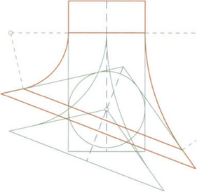
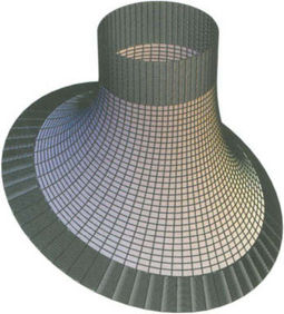
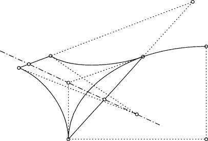
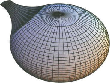
and ![]() are needed from the two surfaces at the ends. We assume that the whole figure should be symmetric with respect to a plane E and the geometric data do so; furthermore a certain shape of the blending surface is wanted. Then one can perform the construction first in that symmetry plane (which plays the same role as E in the example above). But now one has two conic arcs and the control points are already determined by the data. However, also in this case, there must be a central projection with center z on a2mapping the one onto the other; this center is actually the intersection point of the axis a2with E, because all plays in this plane (of course the lines ei = Ei∩ E(i = 1, 2) must intersect at zsince the planes E1 and E2 intersect in a2). However these conditions are not yet sufficient: One has to observe that a central projection in a plane has always a straight line consisting only of fixed points and that the representation of Eq. (23.19) implies that the first axis a1 coincides with it. The following figure shows the details, where the nozzle of a tea pot is designed.
are needed from the two surfaces at the ends. We assume that the whole figure should be symmetric with respect to a plane E and the geometric data do so; furthermore a certain shape of the blending surface is wanted. Then one can perform the construction first in that symmetry plane (which plays the same role as E in the example above). But now one has two conic arcs and the control points are already determined by the data. However, also in this case, there must be a central projection with center z on a2mapping the one onto the other; this center is actually the intersection point of the axis a2with E, because all plays in this plane (of course the lines ei = Ei∩ E(i = 1, 2) must intersect at zsince the planes E1 and E2 intersect in a2). However these conditions are not yet sufficient: One has to observe that a central projection in a plane has always a straight line consisting only of fixed points and that the representation of Eq. (23.19) implies that the first axis a1 coincides with it. The following figure shows the details, where the nozzle of a tea pot is designed.
The tea pot in Figure 23.8 is a rotational ellipsoid. At the front side a skew plane cuts out the bottom of the nozzle, thus having an elliptic cross section. The other end of the nozzle is designed to meet practical as well as aesthetic requirements.
If the construction in the symmetry plane is done, symmetry in space is really attained by taking the second axis orthogonal to that plane; if, additionally, the point z and the vector v(as a point at infinity on a2) are chosen as base points for a2then a trigonometricrepresentation with
is more favorable than that of (23.20) for a closed conic. (Note that sin(φ) occurs only in the coefficient of v.) The coefficients α, … λ are calculated to obtain the proper extensions of the nozzle.
23.5 APPENDIX: STUDYING DUPIN CYCLIDES WITH LIE GEOMETRY
Some of the previous investigations may seem a little bit strange because one can not recognize a unifying principle behind them. Indeed, such a principle exists and is called “Lie geometry” [13] (already mentioned in chapter 3of this book).
The basic idea of Lie geometry is to map the set of all “Lie cycles” L onto a hyperquadric Q lying in the real projective space P5(IR)
and to study configurations in the Euclidean space by looking at their properties in this “model space” of the Lie geometry.
Definition 1
The set L of Lie cycles is the union of the following sets:
1. The set S of oriented spheres inE3,
2. the set U of oriented planes,
The orientation of the spheres is positive, if the normal unit vectors point into the interior; then the radius is assigned a positive value. Otherwise the normal vectors point outwards and the radius is assigned a negative value. Similarly, a certain plane in E3 splits into two different Lie cycles according to the direction of their unit normal vectors.
The mapping (1) is defined separately for each of the different kinds of Lie cycles: For an oriented sphere Sa,r(a being the mid point and r the signed radius according to the orientation) the mapping Λ is given by 17
This definition has to be suitably extended to points and planes: For points simply by setting r = 0 and for planes by passing to the limit r → ∞ thus the image of the plane E … < x, n > − p = 0(with n as oriented normal unit vector) is obtained as
Finally, one defines Λ(∞) = N = (0, 0, 0, 0, 1, 0) IR. This point is called “the north pole” as in Moebius geometry (see chapter 3, section 3.2.2). The north pole is assumed to be different from all other geometric objects, to be incident with any plane but with no sphere. Now one can verify
Theorem 11
For allS ∈ L the images Λ(S) lie on the quadric Q with the equation
and the mapping(23.1) is bijective. Furthermore, let U:= TNQbe the tangent hyperplane to Q at the point N with the equation
then the set U of oriented planes is mapped ontoU {N}. Similarly, letMbe the hyperplane
then Λ(P) = M{N}.
Note that M is not tangent to Q and that, by (4), (5), (6), N is the only common point of U, M and Q . The pole of M will be denoted by P for use later on.
Definition 2
The subgroupLof projectivities ofP5(IR) leaving Q (as a whole) invariant is called the group of Lie transformations (or that of Lie motions). Geometric properties remaining invariant under Lie transformations are called Lie invariant.
The study of Lie invariant properties of figures is called the “Lie geometry” (in the sense of F. Klein’s “Erlanger Programm”). By definition, the quadric Q itself is Lie invariant. It is often called “the absolute quadric of Lie geometry”.
Note that points and planes are not Lie invariant! They can be transformed into any other kind of Lie cycles; only the whole set C of Lie cycles is Lie invariant. Thus the geometric objects U, M, N, P defined above are not Lie invariant but they carry over the Euclidean structure of E3 into the model space. So, if one wants to obtain a Lie invariant property of some configuration F ⊂E3, one has to consider nothing else than the relations of Λ(F) with respect to Q; if, in contrast, one wants to recover a Euclidean property, one has to observe the position of Λ(F) with respect to U, M, N, P. These principles will be exploited in the sequel for the Dupin cyclides.
The Lie geometry can be considered as an extension of the Moebius geometry(with one more dimension): The hyperplane M together with the intersection quadric Q′:= Q∩M is indeed a model space of Moebius geometry, because Q′ has signature (4, 1) and the restriction of the mapping Λ to the points of E3 is given by
with
(set r = 0 in (23.2)). This is just the Moebius mapping if E3 is completed by one point ∞ which is mapped to the north pole (0, 0, 0, 0, 1, 0)IR in M. In this way the Moebius geometry is imbedded into the Lie geometry. In particular, one can choose any 3-space A, different from the tangent space U ∩M at N to Q′(for instance A … ξ4 = 0), and project Q′ from the north pole N onto A (stereographic projection). By this procedure, the Euclidean space E3 is embedded into AU, where the Euclidean structure is conserved (A ∩U plays the role of the “plane at infinity” and A ∩U ∩Q that of the absolute isotropic circle. (See also chapter 3, section 3.2.2)
We mention here without going into the details, that the Laguerre geometry can also be imbedded into the Lie geometry in a similar manner. Thus the Lie geometry contains both and one can show that it is in some sense “the smallest geometry” comprising both the Moebius and the Laguerre geometries. Clearly, Lie geoemtry can also defined (in an analogous manner) for any dimension n ≥ 2; but for the present purpose we confine ourselves to the case n = 3.
Now we come back to the Lie geometry itself and deal with one of its most fruitful notions which is called the “equi-oriented contact of two Lie cycles” and defined as follows:
Definition 3
Two Lie cyclesL1andL2have an equi-oriented contact if and only if one of the following conditions is satisfied:
1. L1, L2 ∈ S ∪ U (two oriented spheres or planes) and they are tangent to each other with both normal vectors pointing into the same direction at the point of contact,
2. L1 ∈ S ∪ U andL2 ∈ E3(one oriented sphere or plane and a point ofE3) and the pointL2is incident with the sphere or planeL1,
3. L1 ∈ U andL2 = ∞ (an oriented plane and the point at infinity have always an equi-oriented contact)
4. L1, L2 ∈ E3 ∪ {∞} andL1 = L2(two points - finite or at infinity - have only an equi-oriented contact if they are coincident).
Now one can prove the following essential property of this notion:
Theorem 12
A pair of Lie cyclesL1andL2has an equi-oriented contact if and only if their Lie images Λ(L1) and Λ(L2) are conjugate (polar) to each other with respect to Q.
Proof: We give the proof only for the case L1, L2∈ S∪E3. Then we have by (2) ![]() and
and ![]() . On the other hand, the polarity condition is by (23.4)
. On the other hand, the polarity condition is by (23.4)
Inserting the above coordinates of Λ(L1), and Λ(L2) yields
This is equivalent to ![]() showing that L1, L2have indeed an equioriented contact.
showing that L1, L2have indeed an equioriented contact.
Observing that any pair of different conjugate points on a quadric (in any projective space) span a line being completely contained in that quadric and vice versa, one recognizes at once:
Theorem 13
Any line1 being completely contained in Q is either the image of a pencil of spheres which are tangent to a plane at a certain point (including these two Lie cycles itself) or the image of a family of parallel planes (with same orientation) completed by the point ∞. The latter case occurs exactly if1 ∈ Uand this implies in addition N ∈ 1.
Now we turn to the Lie-geometric interpretation of surfaces. At any point x(u, v) of a surface one has just such a pencil of tangent spheres that is mapped onto a line 1(u, v) contained in Q. So one has — as the Lie image of a surface F — a line congruence κ, (what means a two-parametric family of straight lines) in the model space. We express this fact simply as κ = Λ(F). But line congruences have, in general, two focal surfaces, generated by the two focal points F1(u, v), F2(u, v) on each line 1(u, v).
With a few lines of calculation (for instance using curvature lines as iso-parameter lines on the surface) one can easily prove:
Theorem 14
The focal points Fion each line1(u, v) of the image Λ(F) of a surface F are the Lie images of the two curvature spheresSi(u, v) at that point of the surface(i = 1, 2).
In particular, for a Dupin cyclide, we know from section 23.2, Theorem 1, that these curvature spheres split into two one parameter families S1: = {S1(u)|u ∈ I1} and S2: = {S2(v)|v ∈ I2} and that, in addition, any sphere of the one family touches any sphere of the other at the corresponding surface point x(u, v). This is an equi-oriented contact if the radius functions are properly signed (see section 23.2.2). Thus the focal surfaces Fi:= {Fi(u, v) | (u, v) ∈ I1× I2} degenerate into two curves quite as those of the normals in the original Euclidean space. However, in the model space, F1(u) must be conjugate to F2(v) because of the equi-oriented contact (Theorem 12). Thus the whole linear subspaces E1and E2spanned by those curves F1and F2respectively are polar to each other with respect to Q. As Fi can not be a line (otherwise Si would be a pencil of spheres) one concludes dim(Ei) ≥ 2 (i = 1, 2). On the other hand, since Q is a non-degenerated quadric in P5(IR) one has dim(E1) + dim(E2) = 4 and this implies dim(Ei) = 2, (i = 1, 2). As the curves Fi are contained in Ei∩Q, they must be conics and we can state:
Theorem 15
The two focal curves F1and F2of the Lie image of a Dupin cyclide are a pair of real non-degenerated conics in two mutually polar planes E1and E2, i.e. Fi = Ei∩Q and E1∩E2 = ∅![]() . Furthermore these focal curves are the Lie images of the two families of enveloping spheres: Λ(Si) = Fi, (i = 1, 2).
. Furthermore these focal curves are the Lie images of the two families of enveloping spheres: Λ(Si) = Fi, (i = 1, 2).
The inverse of this theorem is also true. However one has to include the following three degenerate cases into the notion of a “Dupin cyclide” (which were excluded in section 23.2 by the assumption to be a regular surface):
Theorem 16
(a) Any pair of mutually polar planes each of which intersects the absolute quadric Q in a real non-degenerated conic is the Lie image of a Dupin cyclide (in the sense of the previous theorem).
(b) Each Dupin cyclide is Lie equivalent to any other.
(c) The Dupin cyclide is one of the degenerate cases listed above if and only if E1⊂Uor E2⊂Mor both.
To prove this, one firstly observes that any configuration F1, F2of two conics with the property (a) is projectively equivalent to any other, since the absolute quadric Q — having the signature (4, 2) — can be transformed into the normal form
from which we take that E1defined by η3 = 0, η4 = 0, η5 = 0 and E2defined by η0 = 0, η1 = 0, η2 = 0 is indeed such a configuration F1, F2; thus, there is only one Lie type of it.
The degenerate cases are characterized by the fact that either one of the families of enveloping spheres consists only of planes (Case 1) or the other only of points (Case 2) or both together (Case 3). This proves (c) since planes are mapped into points of U and points of E3 are mapped into points of M.
As mentioned earlier, the different cases of Euclidean preimages of F1, F2are distinguished by the different positions the hyperplanes U and M can have with respect to that configuration F1, F2. For brevity we exclude the degenerate cases from our further investigations.
First we deal with the position of F1, F2with respect to U. This hyperplane intersects the plane Ei in a line 1i. Observing that U is a tangent hyperplane of Q and that Q has signature (4,2), one can find (projective geometry of hyperquadrics) that there are exactly the following two cases:
(A) One of the lines 1i, (i = (1, 2) intersects the corresponding conic Fi = Ei∩Q in a pair of conjugate complex points and the other line 1j intersects Fj = Ej∩Q in a pair of real, different points
(B) 1i is tangent to the conic Fi for both indices i = 1, 2.
Let, in Case (A), F2be the conic with two real intersection points K1, K2with U. The north pole N can not lie on 12(hence in E2) since otherwise E1, being polar to E2, would be contained in U. This would lead to a degenerate cyclide what we had excluded.
But there is the possibility that the line 12meets the line joining N and the pole P of M (since N is in M, P lies in U by main theorem of polar theory).
Thus the Case (A) splits into two subcases
I The line K1K2meets the line NP(or equivalently: the four points K1K2, N and P are contained in a subplane of U).
The Case (B) will be maintained and denoted by (III) in the sequel. Thus we get three main classes of non degenerated Dupin cyclides as in section 23.2.2.
Now we will state that these classes coincide with those of section 23.2.2. As we know, the two families of enveloping spheres are mapped by A onto a pair of mutually polar conics F1, F2. In the Cases (A), (I) and (II), F2intersects U in the pair of real points K1, K2. The preimages of them in E3 are two planes A1and A2which are tangent to all the spheres of S1. Let Ki = (0, ni, pi, 1)IR (see (23.2)), then the condition (I) that PN meets K1K2implies that n1and n2are linearly dependent. So A1and A2are parallel to each other. Hence the cyclide must be rotational symmetric and consequently it is, indeed, a torus (in the sense of section 23.2.2). In the other Case (A), (II), all the spheres of S1are “squeezed” between two intersecting planes, what can not happen for parabolic Dupin cyclides. So the two Cases (II) and (III) correspond to those of section 23.2.2.
The further classification into certain subclasses of (I), (II) and (III) described in section 23.2.2 can be obtained by observing the positions of F1and F2with respect to the hyperplane M. Since, for regular Dupin cyclides, the planes E1and E2are not containedin M (see Theorem 16 (c)), one has also the three possibilities of conjugate complex or coincident or real (different) intersection points of Fi with M. Denoting these three possibilities with the symbols C, T and R respectively, then from the nine combinations of them (for E1and E2independently) there remain only the five cases (CC), (CT), (CR), (TC), (RC) because of the following reason: If there would be a real intersection point Ri of Ei for both the indices then the line joining them (observe that E1and E2are skew, hence R1≠ R2) would completely lie on the intersection quadric Q′:= Q∩M since E1is polar to E2. But this is an oval quadric (see (23.8)) having no lines at all.
Comparing these subcases for instance with those of section 23.2.2, Case (II), one easily realizes that they correspond to the subcase numbers 3, 4, 5, 2, and 1 respectively. In a similar way, the subcases of (I) and (III) can be identified with the remaining possibilities of intersections of E1and E2with M.
So the Lie geometry leads to a complete classification of the Dupin cyclides looking only at the position of F1and F2with respect to the hyperplanes U and M in the model space. Thus Lie geometry is a mean for better understanding the nature of Dupin cyclides.
1. Albrecht, G., Degen, W.L.F. Construction of Béezier rectangles and triangles on the symmetric Dupin horn cyclide by meansof inversion. Computer Aided Geometric Design. 1997;14:349–375.
2. Allen, S., Dutta, D. Supercyclides and blending. Computer Aided Geometric Design. 1997;14:637–651.
3. Allen, S., Dutta, D. Cyclides in pure blending I and II. Computer Aided Geometric Design 1997;14:51–75. Allen, S., Dutta, D. Cyclides in pure blending I and II. Computer Aided Geometric Design. 1997;14:77–102.
4. Allen, S., Dutta, D. Results on nonsingular cyclide transition surfaces. Computer Aided Geometric Design. 1998;15:127–145.
5. Barner, M. Eine differentialgeometrische Kennzeichnung der allgmeinen Dupinschen Zykliden. Aequationes Mathematicae. 1987;34:277–286.
6. Blutel, E. Recherches sur les surfaces qui sont en rnême temps lieux de coniques et enveloppes de cônes du second degré. Ann. sci. école norm, super. 1890;7:155–216.
7. Boehm, W. On cyclides in geometric modeling. Computer Aided Geometric Design. 1990;7:243–255.
8. Boehm, W. Geometric Concepts for Geometric Design. A.K. Peters; 1998.
9. Bol, G. Projektive Differentialeometrie I – III. Wellesley, Massachusetts: Vandenhceck & Ruprecht; 1950–1967.
10. Do Carmo, M.P. Differential Geometry of Curves and Surfaces. Göttingen: Prentice Hall; 1976.
11. Casey, M. On cyclides and sphero-quartics. Philosophical Transactions. 1871;161:585–721.
12. Cayley, A. On the cyclide. Quarterly Journal of Pure and Applied Mathematics. 1873;12:148–165.
13. Cecil, T.E., Dupin submanifolds in Lie sphere geometry. Differential Geometry and Topology, Proceedings Tianjin, 1986–1987. Lecture Notes in Math, 1369. Springer, 1989:1–48.
14. Chandru, V., Dutta, D., Hoffmann, C.M. On the geometry of Dupin cyclides. The Visual Computer. 1989;5:277–290.
15. Degen, W.L.F. Surfaces with a conjugate net of conies in projektive space. Tensor, N. S. 1984;39:167–172.
16. Degen, W.L.F. Die zweifachen Blutelschen Kegelschnittflächen. Manuscripta mathematica. 1986;55:9–38.
17. Degen, W.L.F., Generalized cyclides for use in CAGD. Bowyer A., ed., eds. The Mathematics of surfaces IV. The Institut of Math. & its Applic. Conference Series. Clarendon Press: NY, 1994:349–363.
18. Degen, W.L.F., Nets with plane silhouettes. Fisher R.B., ed., eds. The Mathematics of Surf aces V: Design and Application of Curves and Surfaces. The Institut of Math. & its Applic. Conference Series. Clarendon Press: Oxford, 1994:117–133.
19. Degen, W.L.F. Projektive Differentialgeometrie. In: Giering O., Hoschek J., eds. Geometrie und ihre Anwendungen. Oxford: Carl Hanser Verlag München – Wien, 1994.
20. Degen, W.L.F. Conjugate silhouette nets. In: Cohen A., Rabut Ch., Schumaker L.L., eds. Curve and Surface Design (Saint Malo 1999). Vanderbilt Univ. Press, 2000.
21. W.L.F. Degen Characterizing Dupin cyclides among supercyclides.(In preparation).
22. Dupin, Ch. Applications de Géométrie et de Méchanique. Nashville: Bæchelier; 1822.
23. Dutta, D., Martin, R.R., Pratt, M.J. Cyclides in surface and solid modeling. IEEE Computer Graphics and Applications. 1993;13:53–59.
24. Fladt, A., Baur, K. Analytische Geometrie spezieller Flächen und Raumkurven. Paris: Vieweg & Sohn; 1975.
25. Jessop, C.M. Quartic surfaces with singular points. Braunschweig: Cambridge Univ. Press; 1916.
26. Johnstone, K.J., Shene, C.-K., Dupin cyclides as blending surfaces for cones. Fisher R.B., ed., eds. The Mathematics of Surfaces V: Design and Application of Curves and Surfaces. The Institut of Math. & its Applic. Conference Series. Clarendon Press, 1994:3–29.
27. Johnstone, K.J. A new insertion algorithm for cyclides and swept surfaces using circle decomposition. Computer Aided Geometric Design. 1993;10:1–24.
28. Kaps, M. Teilflächen einer Dupinschen Zyklide in Bézierdarstellung. PhD thesis, TU Braunschweig. 1990.
29. Kummer, E. Über die Fläechen vierter Ordnung, welche eine Doppelcurve zweiten Grades besitzen. Crelles’s Journal f. Mathematik. 1870;69:142–184.
30. R. Krasuaskas. Rational Béezier surface patches on quadrics the torus. Preprint 95-25, Vilnius University.
31. R. Krasuaskas and C Mäurer. Studying cyclides with Laguerre geometry. Preprint no 1974 TU Darmstadt, Fachbereich Mathematik
32. Mäurer, C. Rationale Bézier-Kurven und Bézier-Flächenstücke auf Dupinschen Zykliden. PhD thesis, TU Darmstadt. 1997.
33. Mäurer, C. Generalized parameter representations of tori, Dupin cyclides and supercyclides. In: Le Méehauté A., Rabut C., Schumaker L.L., eds. Curves and Surfaces with Applications to CAGD. Oxford: Vanderbilt Univ. Press; 1997:205–302.
34. Mäurer, C., Krasuaskas, R. Joining cyclide patches along quartic boundary curves. In: Dæhlen M., Lyche T., Schumaker L.L., eds. Mathematical Methods for Curves and Surfaces II. Nashville: Vanderbilt Univ. Press; 1998:359–366.
35. Martin, R.R. Principal Patches for Computational Geometry. PhD thesis, Cambridge University Engineering Departement. 1982.
36. Paluszny, M., Boehm, W. General cyclides. Computer Aided Geometric Design. 1998;15:699–710.
37. Pottman, H., Wagner, M.G. Principal surfaces. In: Goodman T.N.T., Martin R.R., eds. The mathematics of Surfaces VII (IMA Conference at Dundee, 1996). Nashville: Informations Geometers; 1997:337–362.
38. Pratt, M.J. Cyclides in computer aided geometric design. Computer Aided Geometric Design. 1990;7:221–242.
39. Pratt, M.J. The Virtues of Cyclides in CAGD. In: Lyche T., Schumaker L.L., eds. Mathematical Methods in Computer Aided Geometric Design II. Winchester: Vanderbilt Univ. Press; 1992:457–473.
40. Pratt, M.J. Cyclides in computer aided geometric design II. Computer Aided Geometric Design. 1995;12:131–152.
41. Pratt, M.J. Dupin cyclides and supercyclides. In: Mullineux G., ed. The mathematics of Surfaces VI The Institute of Mathematics and its Applications. Nashville: Oxford University Press; 1996:43–66.
42. Pratt, M.J. Quartic supercyclides I: Basic theory. Computer Aided Geometric Design. 1997;14:671–692.
43. Pratt, M.J. On a class of Pythagorean-normal surfaces with planar lines of curvature. In: Crips R.J., ed. The Mathematics of Surfaces VIII, (IMA Conference Birmingham). Oxford: Informations Geometers, 1998.
44. Shene, Ch.-K. Blending two cones with Dupin cyclides. Computer Aided Geometric Design. 1998;15:643–673.
45. Srinivas, Y.L., Dutta, D. Motion planning in three dimensions using cyclides. In: Kunii T., ed. Visual Computing: Integrating Computer Graphics with Computer Vision. Winchester: Springer-Verlag; 1992:781–791.
46. Srinivas, Y.L., Dutta, D. Intuitive procedure for constructing geometrically complex objects using cyclides. Computer-Aided Design. 1994;26:327–335.
47. Srinivas, Y.L., Dutta, D. Blending and joining using cyclides. ASME J. Mech. Des. 1994;116(4):1034–1041.
48. Srinivas, Y.L., Dutta, D. Rational parametric representations of parabolic cyclides: Formulation and applications. Computer Aided Geometric Design. 1995;12:551–566.
49. Srinivas, Y.L., Kumar, K.P., Dutta, D. Surface design using cyclide patches. Computer-Aided Design. 1996;28:263–276.
50. Ueda, K. Normalized cyclide Bézier patches. In: Dæhlen M., Lyche T., Schumaker L.L., eds. Mathematical Methods in CAGD III. Tokyo: Vanderbilt Univ. Press; 1995:1–10.
1In addition, there are some cases of second order cyclides (the natural quadrics) that can be considered as “trivial Cyclides”
2Those of Casey are called “generalized cyclides”
3We wrote here these formulas in an inverse manner using the main curvature radii ri = 1/κ1instead the curvatures κi(i = 1,2) itself, assuming that these quantities do not vanish anywhere. Thus the trivial cyclides, the right circular cones and cylinders, as well as the sphere itself, are excluded in the sequel.
4The curvature spheres are thought to be oriented; a negative radius means that the normal vector points into the interior.
5A regular patch with non-vanishing main curvatures and without umbilics (i.e. ri ≠ 0, (i = 1,2) r1≠ r2) is assumed.
6Later on, when a Dupin cyclide will be considered globally, we will allow spheres to have radius r = 0 (leading to a singular point) or to have radius r = ∞ (then being a plane). In the latter case, the curvature line degenerates into a straight line.
7However, new singularities occur when ![]() or
or ![]() has a zero.
has a zero.
8We keep the denotation f for the abscissa of the focal point though usually denoted by e(the “eccentricity” of the ellipse).
9![]() denotes the closed set of reals
denotes the closed set of reals
10Degenerated Dupin cyclides and a blending along one of the axes of a parabolic cyclide are excluded here.
11The other case that these circles belong to different families seems not to have been considered so far.
12Sabin communicated it to Pratt, who included the result into his paper [38]. The proof was originally given only for cones; later on it was completed by Shene [44] also for the cases of cylinders.
13The case of zero radius, i.e. cones with common apexes is included
14Theorems 3.1 and 3.2 of [2] seem to contradict to this assertion; but that is only caused by the author’s more restrictive definition of a blending.
15One of those blending problems arises from the so-called “Cranfild object”
16This condition is not essential because supercyclides with intersecting axes do exist; they were excluded here only for practical reasons (see [17], [42]).
17The right hand side of the following equation is a class of proportional vectors of IR6, indexed by 0 … 5; the three coordinates of a have to be put at the places 1 … 3.