15.2.1 Notation and terminology

In general, a polynomial in n variables x₁,…, x_n is defined

(15.3)

Each summand is called a term, is a monomial, and c_i is the coefficient of the monomial. By convention, any given monomial occurs in at most one term in a polynomial.

k[x₁,…,x_n] signifies the set of all polynomials in the variables x₁,…,x_n whose coefficients belong to a field k. For example, R[x, y] is the set of all polynomials

(15.4)

where c_i ∈ R and e_1,i,e_2,i ∈ {0,1,2,…}. Thus, “f ∈ R[x,y,z]” means that f is a polynomial whose variables are x, y and z and whose coefficients are real numbers. All polynomials in this chapter have coefficients that are real numbers.

It is often useful to list the terms of a polynomial in decreasing order, beginning with the leading term. This is done using a term order – - a way to compare any two distinct terms of a polynomial and declare which is “greater”.

For linear polynomials, term order amounts to merely declaring an order on the variables. For example, the terms of the polynomial

are in proper order if we declare x > y > z. If we declare y > z > x, the proper order would be 3y−4z+2x. For non-linear polynomials, we begin by declaring an order on the variables, and then we must also choose one of several schemes that decide how the exponents in a polynomial influence term order. One such scheme is called lexicographical order (nicknamed lex), defined as follows. If the variables of a polynomial are ordered x₁ > x₂ > … > x_n, then given two distinct terms and if

For example, the polynomial

using lex with x > y > z would be written 5x³z + 3x²y²z + 4xy³z² + 7xz³ + 6y² + 8 and its leading term is 5x³z. Using lex with z > x > y it would be written 7z³x + 4z²xy³ + 5zx³ + 3zx²y² + 6y² + 8 and the leading term would be 7z³x. Or using lex with y > z > x it would be written 4y³z²x + 3y²zx² + 6y² + 7z³x + 5zx³ + 8 and the leading term would be 4y³z²x.

Another choice for term order is the degree lexicographical order (abbreviated deglex). If the variables are ordered x₁ > x₂ > … > x_n, then using deglex, T_i > T_j if

Using deglex with x > y > z, the terms of 3x²y²z + 4xy³z² +5x³z + 6y² + 7xz³ + 8 would be ordered 4xy³z² + 3x²y²z + 5x³z + 7xz³ + 6y² + 8.

As observed in the lex and deglex examples, term orders ignore the coefficient of a term, so a term order might more properly be called a monomial order.

Other term orders can also be defined, such as degree reverse lexicographical order. The precise requirements for any term order are discussed in reference [6], page 18.

The n-dimensional real affine space is denoted Rⁿ and is the set of n-tuples:

(15.5)

15.2.2 Ideals and varieties

The polynomial ideal generated by f_i, …, f_s ∈ k[x₁, …, x_n], denoted <f₁, …, f_s>, is defined

The polynomials f₁, …, f_s are called the generators of this ideal.

Consider a set of polynomials f₁, f₂, …, f_s ∈ k[x₁, …, x_n]. Let (a₁, …, a_n) be a point in kⁿ satisfying f_i((a₁, …, a_n) = 0, i = l, …, s. The set of all such points (a₁, …, a_n) is called the variety defined by f₁, …, f_s, and is denoted by V(f₁, …, f_s):

(15.6)

A variety defined by a single polynomial—called a hypersurface—is the most familiar instance of a variety. A hypersurface in R² is a planar curve defined using an implicit equation, and a hypersurface in R³ is what is normally called an implicit surface in CAGD. For example, V(x²+y² - l) is a circle defined in terms of the implicit equation x²+y²−1 = 0 and V(2x + 4y - z + 1) is the plane whose implicit equation is 2x + 4y - z + 1 = 0.

A variety V(f₁, …, f_s) defined by more than one polynomial (s > 1) is the intersection of the varieties V(f₁) … V(f_s).

15.2.3 Gröbner bases

It can be very useful to devise alternative generators for an ideal. Necessary and sufficient conditions for <f₁, …, f_n > = <g₁, …, g_m > are f₁, …, f_n ∈ {g₁, …, g_m} and g₁, …, g_m ∈ {f₁, …, f_n}.

A Gröbner basis of an ideal I is a set of polynomials {g₁, …, g_t} such that the leading term of any polynomial in I is divisible by the leading term of at least one of the polynomials g₁, …, g_t. This, of course, requires that a term order be fixed for determining the leading terms: different term orders produce different Gröbner bases. Several excellent books have been written on Gröbner bases that do not presuppose that the reader has advanced training in mathematics [6],[10],[17]

A Gröbner basis is a particularly attractive set of generators for an ideal, as illustrated by two familiar examples. If {f₁, …, f_s} are polynomials in one variable, the Gröbner basis of <f₁, …, f_n> consists of a single polynomial: the greatest common divisor (GCD) of f₁, …, f_s. If {f₁, …, f_n} are linear polynomials in several variables, the Gröbner basis is an uppertriangular form of a set of linear equations. The Gröbner basis of these special cases provides significant computational advantage and greater insight, and the same is true of the Gröbner basis of a more general ideal.

Gröbner bases are the fruit of Bruno Buchberger’s Ph.D. thesis [12], and are named in honor of his thesis advisor. Buchberger devised an algorithm for computing Gröbner bases [13],[17],[18]. Also, commercial software packages such as Maple and Mathematica include capabilities for computing Gröbner bases.

15.3.1 Sylvester’s resultant

Consider the two polynomials

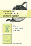
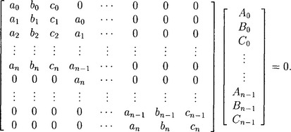
Using Sylvester’s dialytic method, we multiply f(t) by t^m−1, t^m-2, …, t, 1 and g(t) by tⁿ⁻¹, …,t, 1, arriving at m + n polynomials, which can be arranged in matrix form:

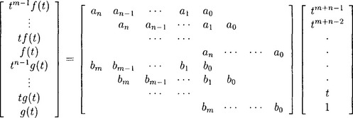
The determinant of the coefficient matrix is known as Sylvester’s resultant for f(t) and g(t). The ideal generated by these m + n polynomials is just the ideal <f(t),g(t)>. Thus they have the same variety. When there exists one value of t in the variety, Sylvester’s resultant must vanish.

Sylvester’s resultant can also be derived using a method invented by Euler. Euler introduced two polynomials h(t) of degree m − 1 and k(t) of degree n −1 with coefficients undetermined. Letting h(t)f(t) - k(t)g(t) = 0 leads to m + n linear equations with m + n unknowns which are the coefficients of h(t) and k(t). The determinant of the coefficient matrix of these m + n linear equations is exactly Sylvester’s resultant. Obviously the determinant vanishes if and only if there exist nonzero polynomials h(t) of degree not greater than m − 1 and k(t) of degree not greater than n − 1 such that h(t)f(t) = k(t)g(t) holds. This is equivalent to the existence of the common roots of polynomials f(t) and g(t). Therefore Euler’s method shows that R(f,g) = 0 is not only the necessary but also sufficient condition for f(t) and g(t) to have common roots.

15.3.2 Bezout’s resultant

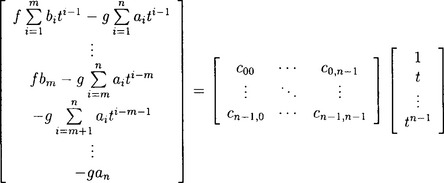
Another popular resultant formulation for two univariate polynomials is Bezout’s resultant. A nice derivation of Bezout’s resultant is due to Cayley. Without loss of generality, we assume the degree of the polynomial g(t) is less than the degree of f(t), i.e., m ≤ n. Construct a symmetric function

Some algebraic manipulation shows that δ(t, s) is a degree n − 1 polynomial in s whose coefficients are polynomials of t:

The variety of the ideal generated by these n polynomials is the same as V(<f(t), g(t)>). Write these polynomials in matrix form:

with the entry and the convention that b_m+1 = … = b_n = 0.

This coefficient matrix is called Bezout’s matrix. If V(<f,g>) is non-empty, the determinant of Bezout’s matrix must vanish. The converse is also true when n = m, the proof of which can be found in [22],[26]. The determinant is therefore a resultant for f and g, known as Bezout’s resultant. In general, Bezout’s resultant has dimension n × n while Sylvester’s resultant has dimension (n + m) × (n + m).

When n > m, Bezout’s determinant has an extraneous factor of a_n^n-m. This extraneous factor can be removed by modifying Bezout’s resultant as follows [19]: The first mpolynomials are the same as in (15.7); and the remaining n - m polynomials are obtained from t^i-m g(t), i = m, …, n. Thus C_ij = b_i+j-m for i ≥ m, 0 ≤ j ≤ n − 1. Look at the example of f(t) = a₂t² + a₁t + a₀ and g(t) = b₁t + b₀. The original Bezout’s determinant is

and the variant of Bezout’s resultant is .

15.3.3 Dixon’s resultant

Cayley’s formulation can be extended to the case of three bivariate polynomials. Consider three polynomials:

Dixon observed that the expression

is actually a polynomial of degree 2n − 1, m − 1, n − 1 and 2m − 1 in s, t, α, β respectively. Thus it can be written as where d_ijkl are expressions in a_ij,b_ij and c_ij.

For any (s, t) ∈ V(<f,g,h>), δ(s,t,α,β) vanishes no matter what α and β are. Thus the coefficients of each α^kβ^l must vanish at these (s, t) pairs. This gives 2mn polynomials, each of which has 2mn terms in s and t since s has degree 2n − 1 and t is degree m − 1. The determinant of the coefficient matrix from these polynomials serves as a resultant for f, g and h, called Dixon’s resultant [23].

Consider the example:

Dixon’s method gives

where (ij,kj,pq) stands for the 3 × 3 determinant .

15.4.1 Resultant-based method

We have presented the resultant tool for determining whether two polynomials have a common root. We now apply that tool to converting the parametric equation of a curve given by (15.1) into an implicit equation of the form f(x,y) = 0.

We proceed by forming two auxiliary polynomials:

View g(x, t) as a polynomial in t whose coefficients are linear in x, and view h(y, t) as a polynomial in t whose coefficients are linear in y. If we compute the resultant of g(x,t) and h(y,t), we do not arrive at a numerical value, but rather a polynomial in x and y which we call f(x,y). Note that g(x,t) = h(y,t) = 0 only for values of x,y and t which satisfy the relationships x = a(t)/c(t),y = b(t)/c(t). Clearly, for these values of x,y and t, the resultant f(x,y) must vanish. Conversely, any (x,y) pair for which f(x,y) = 0, causes the resultant of g and h to be zero. But, if the resultant is zero, then we know that there exists a value of t for which g(x, t) = h(y, t) = 0. In other words, all (x, y) for which f(x,y) = 0 lie on the parametric curve and therefore f(x,y) = 0 is the implicit equation of that curve.

As discussed, the resultant is the determinant of a matrix of coefficients for a set of polynomials. Inversion—computing the parameter t for a point (x, y) known to lie on the curve—can be performed by solving such a set of polynomial equations using Gauss elimination or Cramer’s rule.

We illustrate with the circle parametrized by (15.8). We have

Using Sylvester’s resultant, we obtain a 4 × 4 determinant

Bezout’s resultant provides a 2 × 2 determinant

We could obtain an inversion equation by solving the equations:

from which t = y/(x + 1) or t = (1 − x)/y.

Two remarks should be made. First, if a(t),b(t) and c(t) in (15.1) are not relatively prime, the common factor should be removed before the resultant method is applied. Otherwise, the resultant will be identically zero, containing no information about the curve, since p and q have always common solutions for arbitrary (x, y) pair. Second, if the degrees of p(x, t), q(y, t) with respect to t are not the same, the variant of Bezout’s resultant is used.

15.4.2 Gröbner basis technique

In order to use Gröbner basis method for implicitizing a rational parametric curve defined by (15.1) with GCD(a(t),b(t),c(t)) = 1 (otherwise, the common factor can be removed), we define the ideal

(15.9)

If f(x,y) = 0 is the implicit equation of (15.1), then f ∈ I ∩ R[x,y]. To guarantee f appears in the Gröbner basis, we order the variables t > x > y, and then construct the Gröbner basis with the lexicographic ordering for the ideal I. The lexicographic ordering results in a Gröbner basis that has a triangular structure. Thus the Gröbner basis obtained will contain the curve’s implicit form—an element which does not involve t, and an inversion—an element which is linear in t.

In the example of the circle (15.8), I = <(1 + t²)x − (1 − t²), (1 + t²)y - 2 t>. Using the computer algebra system MAPLE, we obtain the Gröbner basis I = {- y + x + tx,x − 1 + yt,y² + x² − 1). Therefore the polynomial y² + x² − 1 gives the implicit equation x² + y² − 1 = 0. The two other polynomials - y + x + tx and x − 1 + yt are linear in t and thus provide the inversion t = y/(1 + x) or t = (1 − x)/y.

15.4.3 Moving curve technique

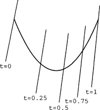
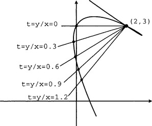
A recent development in impliciting a planar rational parametric curve is the “moving curve” method [19],[42],[44]. A moving curve is defined as

where f_i(x,y,w) is a homogeneous polynomial of degree d. Thus C(x,y,w;t) = 0 is a family of algebraic curves, with one curve corresponding to each t. In particular, when d = 1, C(x,y,w;t) = 0 is a family of implicitly defined lines. Therefore we call it a moving line of degree m. Likewise, C(x, y, w; t) = 0 is called a moving conic of degree m when d = 2. A moving curve C(x, y, w; t) = 0 is said to follow a planar rational curve (15.1) if C(a(t), b(t), c(t); t) is identically zero, that is, if for all values of t, the point (a(t)/c(t),b(t)/c(t)) lies on the moving curve C(x,y,w;t) = 0. For example, each row of Bezout’s matrix or Sylvester’s matrix corresponds to a moving line following the curve. Figure 15.1 illustrates a parametric curve and a few moving lines.

The moving curve technique identifies m + 1 independent moving curves that follow a given rational curve. A square matrix can then be formed from the coefficients of these moving curves with respect to t and the determinant of the matrix gives the desired implicit equation. In general, such a collection of moving curves can be found by solving a set of linear equations [43]. For example, a degree n − 1 moving line

(15.10)

follows a rational curve (15.1) if

which can be expressed as 2n linear equations with 3n unknowns

where a_i,h_i,c_i are the coefficients of the polynomials a(t), b(t),c(t). Thus solving the equations for A_i,B_i,C_i yields n linearly independent moving lines of degree n − 1 that follows the curve.

Recently the problem of finding an appropriate set of moving lines was illuminated by the description of the μ-basis [19]. A μ-basis for a degree-n planar rational curve consists of two moving lines p(x, y; t) and q(x, y; t), of degree p and n - p respectively, which form an ideal basis for all moving lines that follow the curve. An efficient method of computing the μ-basis is given in [52]. Once the μ-basis of a curve is known, the problem of finding m + 1 linearly independent moving curves is greatly simplified. For example, consider the degree four curve:

This curve has a μ-basis of

Thus four moving lines of degree 3 are p,t p,q, t q. Moreover, two moving conics of degree 1 can be obtained by taking Bezout’s resultant of p and q. Each row in Bezout’s matrix corresponds to a moving conic. Therefore the implicit equation can be expressed as a 2 × 2 determinant whose elements are quadratic in x and y. In general, for a degree n rational curve, using a variant of Bezout’s resultant on the μ-basis, we can write the implicit equation of the rational curve as the determinant of an (n - p) × (n - p) matrix with μ rows whose elements are quadratic in x and y, and the remaining n − 2μ rows with elements linear in x and y, while conventional implicitization methods generate the determinant of an n × n matrix [22],[34].

15.5.1 Planar algebraic curves

Implicitization shows that a degree n parametric curve can be represented using a degree n implicit equation. Any implicit equation that can be obtained by implicitizing a parametric curve is said to be rational (in other words, a rational curve is any curve which can be parametrized using rational functions). All algebraic quadratic curves have rational quadratic parametrizations, whereas algebraic curves of degree greater than two are not generally rational.

A degree n algebraic curve is defined by a degree n polynomial f(x,y), which has (n + 1)(n + 2)/2 terms. For example, a degree two algebraic curve has six terms: a₁x² + a₂xy + a₃y²+a₄x+a₅ y+a₆ = 0. However, any one coefficient can be specified by scaling all of the other coefficients. (For example, the coefficient of x² in the quadratic example can be set to 1 by dividing all the coefficients by a₁). Thus, there is an (n + l)(n + 2)/2 − 1 = n(n + 3)/2 dimensional family of degree n algebraic curves. Geometrically, this means a degree n algebraic curve can be forced to interpolate n(n + 3)/2 points in general position.

The parametric equation of a rational degree n curve has 3(n + 1) coefficients. However, any one of these can be specified by scaling all of the other coefficients. Also, three other coefficients can be specified by changing the parametrization by a rational linear transformation , and consequently there is a 3n − 1 dimensional family of degree n rational curves.

15.5.2 Genus and rationality

The condition under which an implicit algebraic curve can be parametrized using rational polynomials is that its genus must be zero [49]. Basically, the genus of a curve is given by the formula g = (n−1)(n−2)/2 - d where g is the genus, n is the degree, and d is the number of double points. There are some subtleties involved in this equation if the singularities are not simple double points, but we will not concern ourselves with them.

A double point on a curve is a point for which f(x,y) = f_x(x,y) = f_y(x,y) = 0 where the subscripts x and y denote partial differentiations, and for a point of multiplicity k, all partials up to order k − 1 vanish. Geometrically, a double point means that any straight line through it intersects the curve at least twice at this point.

We see immediately that all curves of degree one and two have genus zero and thus can be parametrized using rational polynomials. A degree three algebraic curve is rational only if it has a double point.

An irreducible curve is one whose implicit equation f(x, y) = 0 cannot be factored. Rational curves (that can be parametrized using a single parametric equation) are irreducible, and an irreducible curve of degree n can have at most (n − l)(n − 2)/2 double points. Thus, a rational curve has the most double points possible for a curve of its degree.

15.5.3 Parametrizing curves

One way to parametrize a degree two algebraic curve is to transform the conic into the standard form which has already a parametrization, and then to transform the standard parametrization back. The standard equations of conics are: = 1 for an ellipse, for a hyperbola, and y² = 2px for a parabola. They can be parametrized as and , respectively. Therefore the main step is to find a nonsingular affine coordinate transformation. This can be carried out as follows.

Suppose the conic equation is Ax² + 2Bxy + Cy² + 2Dx + 2Ey + F = 0. First we convert the equation into the form

(15.12)

If B = 0, it is done. If A = C = 0 and B ≠ 0, then set .

Otherwise, if A ≠ 0, B ≠ 0, then

Thus we only need to set . A similar transformation can be derived if C ≠ 0 and B ≠ 0.

Second, if one of and in (15.12) is zero, the curve is a parabola. Assume that ≠ 0 and = 0. Then . Thus setting

arrives at the standard parabola equation. A similar process deals with the case of = 0, ≠ 0. If both of and are nonzero, we have .

Therefore we can take a translation of to make the curve equation in the standard form. Composing the transformations in the above two steps gives the required coordinate transformation.

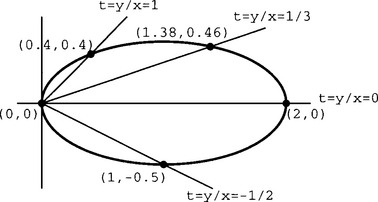
Another method to parametrize a conic is to establish a one-one correspondence between points on the curve and a family of lines through a point on the curve, which is called a pencil-of-lines. This pencil-of-lines method is most easily illustrated by translating the curve so that it passes through the origin, such as does the curve

which is an ellipse centered at (1,0). We next make the substitution y = tx and solve for x as a function of t: x²(l + 4t²) − 2x = 0. Then

Notice that y = tx is a family of lines through the origin. The variable line y = tx intersects the curve once at the origin, and at exactly one other point (because of Bezout’s theorem: two algebraic curves of degree m and n intersect at either mn points or else they have common components [49]). Thus, we have established a one-one correspondence between points on the curve and values t which correspond to lines containing that point and the origin. The ellipse parametrized in this manner is shown in Figure 15.2.

To parametrize a genus zero cubic curve, one must first find its double point, which is done by solving h(x, y) = h_x(x, y) = h_y(x, y) = 0. Once the location of the double point is determined, one can translate the curve so that the double point lies on the origin. Then the same trick in the pencil-of-lines approach for conics can be played with this cubic curve since the curve now has an equation involving terms of degree two and three only.

Consider this example of the cubic curve

for which

and

We compute the x coordinates of the intersections of f_x = 0 and f_y = 0 by taking the resultant of f_x and f_y with respect to y:

whose roots arex = 2 and Likewise the y coordinates of the intersections of f_x = 0 and f_y = 0 are found by taking the resultant of f_x and f_y with respect to x:

whose roots are y = 3 and ¿From these clues, we find that the only values of (x,y) which satisfy f(x,y) = f_x(x,y) = f_y(x,y) = 0 are (x,y) = (2,3). This is therefore the double point.

The double point can also be found by computing the Gröbner basis of <f, f_x, f_y > using lex ordering with x > y, the Gröbner basis is {x − 2, y − 3}.

This curve can be parametrized by translating the implicit curve so that the double point lies at the origin. This is done by making the substitution , yielding

Parametrization is then performed using the method discussed earlier in this section,

and the parametrized curve is translated back so that the doubled point is again at (2, 3) (see Figure 15.3):

For a general algebraic curve, the parametrization problem involves two steps: determine whether it admits a rational parametric representation, and find one if so. The algorithms, in general, are not as simple as for conics or cubics. [References 1–4],[47] provide various computational techniques for parametrizing algebraic curves.

15.6.1 Parametric curve and implicit curve

Given one curve defined by the parametric equation (x, y) = (x(t),y(t)) and a second curve defined by the implicit equation f(x,y) = 0, we replace all occurrences of x and y in the implicit equation by x(t) and y(t), respectively. These substitutions create a polynomial f(x(t),y(t)) = g(t) whose roots are the parameter values of the intersection points. The (x, y) coordinates of these intersection points can be easily obtained by substituting the parametric values into the equation of the parametric curve.

15.6.2 Implicit curve and implicit curve

For two algebraic curves f₁(x,y) = 0 and f₂(x,y) = 0, the problem of computing the intersection amounts to computing the variety V(f₁,f₂).

One direct method for computing the variety V(f₁,f₂) is to take the resultant of f₁ and f₂ with respect to x or y. The x-resultant is computed by treating f₁ and f₂ as polynomials in x whose coefficients are polynomials in y. The x-resultant eliminates x and produces a polynomial in y whose roots are the y coordinates of the intersection points.

We illustrate with a circle 6x² + 6y² − 2x − 15y − 4 = 0 and a hyperbola x² - y² − 1 = 0 (see Figure 15.4).

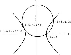
The x-resultant of these two implicit equations is 144y⁴ − 360y³ + 269y² − 60y whose roots are y = 0, y = 4/3, y = 3/4, and y = 5/12. These are the y-coordinates of the points of intersection of the two curves.

We can use the y-resultant to find the x-coordinates of the points of intersection. The y-resultant is 144x⁴ − 48x³ − 461x² + 40x + 325 which has roots x = 1, x = 5/3, x = −5/4, and x = −13/12.

We now know the x and y components of the points of intersection, but we don′t know which x goes with which y! One way to determine that is simply to evaluate each curve equation with every x and every y to see which (x, y) pairs satisfy both curve equations simultaneously. A more clever way is to use Euclid’s algorithm which computes the GCD of two polynomials. In fact, Euclid’s algorithm spares us the trouble of computing both the x-resultant and the y-resultant.

Suppose we had only computed the y-resultant and we wanted to find the y-coordinate of the point of intersection whose x-coordinate is 5/3. That is to say, we want to find a point () which satisfies both curve equations. We substitute x = 5/3 into the circle equation to get 16/6 - y² = 0 and into the hyperbola equation to get 6y² − 15y + 28/3 = 0. We now simply want to find a value of y which satisfies both of these equations. Euclid’s algorithm tells us that the GCD of these two is 3y − 4 = 0, and thus one point of intersection is ().

Gröbner bases also provide a systematic computational method with the assurance that all intersection points have been found. The general strategy is based on the simple observation that V(f₁, …, f_s) = V(<f₁, …, f_s>). Consequently, if f₁, , f_s and g₁ …, g_t are generators of the same ideal, then

Consider the previous example of a circle V(6x² + 6y² − 2x − 15y − 4) and a hyperbola V(x² - y² − 1). It can be verified that

(the Gröbner basis)

Since any point of intersection must be zeros of all generators of the ideal, the only possible x-coordinates for the intersection points must be roots of 144x⁴ − 48x³ − 461x² + 40x + 325 = 0 (the roots are , − and −). The corresponding y coordinates can then be solved using −12x² + 2x + 15y + 10 = 0.

15.6.3 Parametric curve and parametric curve

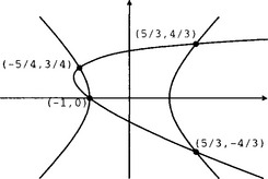
If we begin with two parametric curves, we can first implicitize one of them, and then use the substitution method to compute the intersection points. We illustrate this process by intersecting the curve

with the curve

(see Figure 15.5). The two curves intersect four times, which is the most that two quadratic curves can intersect. We implicitize the first curve and get the implicit equation x² - y² − 1 = 0. Substituting the parametric equation of the second curve into this implicit equation and clearing the denominator, we arrive at the intersection equation:

We now compute the roots of this degree four polynomial, which are 23, 1/3, 19/6 and − 1. These are the parametric values on the second curve for the intersection points. From the parametric equation of the second curve, the corresponding (x, y) coordinates can be easily found: (5/3, 4/3), (−1, 0), (−5/4, 3/4), (5/3, −4/3). The parametric values on the first curve for the intersection points can be found from the inversion formulas s = y/(1 − x) and s = -(1 + x)/y. They are −2, 0, 1/3 and 2, respectively.

Tests indicate that this implicitization-based intersection algorithm is several times faster than subdivision methods for quadratic and cubic curves, but subdivision methods are faster for curves of degree five and greater [38].

Gröbner bases and resultants can also be used for finding the intersections between two parametric curves. The intersections of the curves (x,y) = (a₁(s)/c₁(s),b₁(s)/c₁(s)) and (x,y) = (a₂(t)/c₂(t),b₂(t)/c₂(t)) satisfy

This prompts us to compute the variety V(a₁(s)c₂(t) - a₂(t)c₁(s),b₁(s)c₂(t) - b₂(t)c₁(s)) in the (s, t)-space. The methods discussed in section 15.6.2 can then be employed. For the previous example, the Gröbner basis using lexicographic ordering with t > s is

Solving the third polynomial in the Gröbner basis gives six roots: 0, 1, 2, 1/3, −2, −1. Note that the solutions of 1 and −1 are actually the roots of the denominator 1 - s² of the first curve, and thus should be discarded. We then substitute the rest four roots into the second polynomial in the Gröbner basis and solve for the corresponding values of t. These values of s and t are the parametric values of the intersection points on the first and second parametric curves.

15.7.1 Implicit degree of a rational parametric surface

The implicit degree can be thought of as the number of times that the surface is intersected by a generic straight line [15],[48]. Define a generic straight line as the intersection of two distinct planes in general position a₁x + a₂y + a₃z + a₄ = 0 and b₁x + b₂y + b₃z + b₄ = 0. The planes intersect the parametric surface (15.2) in curves

(15.13)

and

(15.14)

These curves are each degree n in s, t. By Bezout’s theorem, these two curves intersect in n² points, which must also be the number of times that the straight line common to the two planes intersects the surface. Thus, the degree of the surface, and of its implicit equation, is n².

It seems curious that there are gaps in the sequence of the implicit degrees of parametric surfaces: 1, 4, 9, …. Are there no parametric surfaces whose implicit degree is 3 or 5 for example, or under what conditions will the degree decrease?

It may happen that there are values s_b and t_b satisfying a(s_b, t_b) = b(s_b, t_b) = c(s_b, t_b) = d(s_b, t_b) = 0. These parameter pairs (s_b, t_b) are referred to as base points. If a base point exists, the intersection curve of any plane with the surface will contain the base point. Thus, the above two curves will intersect at the base point and at n² − 1 other points. However, since the base point does not map to a unique point on the surface (x = y = z = 0/0 is undefined), this does not represent a point at which the straight line intersects the surface, and the degree of the surface is therefore n² − 1. Each additional simple base point diminishes the degree of the surface by one. Base points at infinity occur when all plane sections have a common asymptotic direction.

To understand the influence of more complicated base points on the implicit degree, consider the linear system of all curves given by (15.13), where each curve in the linear system is the intersection of the surface with the plane a₁x + a₂y + a₃z + a₄ = 0. A base point is any point in common with all members of the linear system. If two general curves in the linear system are tangent at a base point, they intersect twice at the base point and the degree of the surface becomes n² − 2. If two general curves in the linear system have a double point in common, they intersect four times at that base point and the degree becomes n² − 4. Thus, a general degree formula is n² - ρ where ρ is the total number of times that two general curves in the linear system intersect at base points. This also assumes that the surface has a one-to-one parametrization.

If the surface (15.2) is a tensor product surface—one of the most popular representations for surfaces in CAGD—the parametrization is a bi-degree (n_s,n_t) parametrization in s and t. That means, n_s and n_t are the highest degrees of the parametric equations with respect to s and t. In this case, the total parametric degree is n = n_s + n_t. But there exist two base points at infinity, corresponding to s = 00, t = 00, counted at least n_t² and n_s² times respectively [14]. Thus the implicit degree of a bi-degree (n_s,n_t) parametrized rational surface is at most (n_s + n_t)² - n_s² - n_t² − 2n_sn_t. For example, a bicubic surface is usually of implicit degree 18.

15.7.2 Surface intersection curves

Surface/surface intersection (i.e., finding the intersection curve of two surfaces) is an important geometric operation in CAGD. The usual approach is to compute an approximation for the intersection curve. Algebraic geometry provides important information on the nature of intersections of parametric surfaces. For example, the degree of the intersection curve is easy to determine using Bezout’s theorem which states that two surfaces of degree m and n respectively intersect in a curve of degree mn. Therefore if two surfaces have implicit degree n₁ and n₂, the intersection curve has a degree n₁n₂ (unless the surfaces have common components). Thus, two bicubic patches generally intersect in a curve of degree 324.

15.7.3 Implicitization

Resultants can be used to implicitize a rational parametric surface. Dixon’s resultant is a good choice, because it works on three polynomials in two variables. Given a rational parametric surface (15.2), construct three auxiliary polynomials:

Note that p(x,s,t) = q(y,s,t) = h(z,s,t) = 0 only for values of x,y,z and s,t which satisfy (15.2). View p(x,s,t), q(y,s,t) and h(z,s,t) as polynomials in s and t whose coefficients are linear in x, in y and in z, respectively. Then applying Dixon’s resultant to these polynomials to eliminate s and t, we obtain a polynomial in x, y and z which we denote f(x, y, z). Thus f(x, y, z) = 0 defines the implicit equation of the rational surface. In addition, by Cramer’s rule, taking the ratio of the determinants of the submatrices from the Dixon’s matrix corresponding to the terms sⁱ t^j and sⁱ⁻¹t^j, or the terms sⁱ t^j and sⁱ t^j−1 yields the inversion equations of s = sⁱ t^j/sⁱ⁻¹t^j and t = sⁱ t^j/sⁱ t^j−1. Unfortunately, if the surface has finite basepoints, the resultant is identically zero and the algorithm fails.

The implicitization of rational parametric surfaces can also be accomplished by computing the elimination ideal. The Rational Implicitization Theorem [17] states that if J = 〈dx - a, dy - b, dz - c, 1 - dw〉, then V(J ∩ R[x, y, z]) is the smallest variety in R³ containing the parametric surface. The polynomial 1 - dw is introduced to assure that the method will work even if base points are present. Otherwise, base points would cause J ∩ R[x,y,z] = {0}. In practical computation, we construct the Gröbner basis with the lexigraphic ordering for the ideal J with s > t > x > y > z. The Gröbner basis will contain a polynomial in x,y,z. This is the implicit equation. If the parametrization of the surface is a one-to-one map, two polynomials linear in t and s are also contained in the Gröbner basis. They can produce the inversion maps.

Notwithstanding the robustness and elegance of the Gröbner basis solution to surface implicitization, it is not very computationally efficient. Recently, a promising new method, called the moving surface method, has been proposed for implicitizing rational surfaces [43]. Like resultants, the implicit equation is expressed as the determinant of a matrix.

We define a moving surface as

where the equations f_i(x, y, z) = 0, i = 1, σ define a collection of implicit surfaces and where the γ_i(s, t), i = 1, …, σ are a collection of polynomials in s and t. We require the γ_i(s, t) to be linearly independent and to be relatively prime. A moving surface is said to “follow” a rational parametric surface (15.2) if

If we can find a set of σ moving surfaces

each of which follows a given rational surface, then

gives the implicit equation — as long as the degree of f(x, y, z) is equal to the degree of the implicit equation of the rational surfaces.

In comparison, Gröbner basis method theoretically provides an elegent solution to implicitization of parametric surfaces, but involves a huge computation which limits its use in practice. The method of resultants is efficient, but fails when base points occur. Multivariate resultants can also be used for implicitization [15]. The moving surface method actually simplifies in the presence of base points. Furthermore, the method of moving surfaces provides a very compact representation for the implicit equation of a surface. For example, a bicubic patch can, in general, be written as a 9 × 9 determinant whose elements are all degree two in x,y,z. By contrast, Dixon’s resultant produces an 18 × 18 determinant. However, further study is needed on the moving surface method.

In summary, the operation of surface implicitization has not yet gained widespread use in practice, partly because the degree explosion that one encounters when moving from the parametric to the implicit form counteracts most algorithmic advantages that the implicit form might have over the parametric, and also because the computational complexity is very large, especially in the event of base points.

15.7.4 Parametrizaion

For an algebraic surface of arbitrary degree, Castelnuovo gave a necessary and sufficient condition for the existence of the rational parametrization [51]. Unfortunately, this criterion does not provide a constructive approach to parametrization. A systematic method for parametrizing a general rational algebraic surface is under investigation. Recently, various computational algorithms for parametrizing certain lower degree algebraic surfaces have been developed.

All degree two surfaces are rational. We can parametrize a quadric surface much like we did for conics. For example, we can use a pencil-of-lines approach by first translating the surface so that it touches the origin. Then define a line through the origin as the intersection of two pencils of planes: y = sx and z = tx, say, and intersect the surface with that line. We demonstrate the procedure with a sphere x² + y² + z² − 2z = 0. Substituting y = sx and z = tx, we obtain x²1 + s² + t²) − 2tx = 0. This gives the x coordinates of the two points where the line intersects the sphere. Discarding the intersection at the origin gives the parametrization

Most cubic surfaces are also rational. The only exception is the ruled cubic generated by a non-rational cubic curve. The cubic surface has a fascinating geometry. For example, the general cubic surface contains 27 straight lines, and those lines can be used in determining a parametrization for the surface. A detailed discussion can be found in [9],[39],[41].

• A curve or a surface is said to be properly parametrized if to each point on the curve, except for possibly a finite number of points, there corresponds only one parameter value. It is natural to ask whether any improperly parametrized curve or surface can be reparamtrized to become properly parametrized. For a rational curve, a classical theorem due to Lüroth guarantees the existence of a reparametrization [49]. However, for a rational surface, it depends on the base field where the surface is defined. Gröbner basis methods can be used for detecting and correcting improper parametrization [24].

• Geometric continuity was originally introduced as a smoothness measure for parametric curves and surfaces. This concept is also meaningful for implicit curves and surfaces. The geometric continuity conditions for implicit surfaces is studied in [25]. This consideration is important when using algebraic surfaces in geometric modeling. One application is to construct blending algebraic surfaces with a specified continuity [50]. Algebraic surfaces have been shown to have advantages over parametric surfaces when performing the blending operation.

• The fact that the most popular free-form surface patches – bicubic patches – are actually algebraic degree 18 has tempted some researchers to investigate the possibility of using lower degree algebraic surfaces for modeling purposes. Surfaces in algebraic geometry are usually global in nature while surfaces in CAGD are usually finitely defined (i.e., patches). The main reasons that parametric surface patches have been so popular in CAGD are that they can be pieced together with any desired degree of continuity, and that there exist many elegant, intuitively meaningful techniques for controlling their shape. Therefore, to make algebraic surfaces useful in CAGD, the Bernstein-Bézier techniques have been adapted in defining algebraic surfaces [36]. Meaningful and efficient methods, such as interpolation, least-squares approximation and interactive modification, have been developed to model complicated shapes using piecewise implicit algebraic surfaces [7],[8],[20],[21].

• Algebraic tools such as resultants and discriminants can help compute the intersection points between a ray and a surface (useful for performing ray tracing), and can help compute the silhouette points or curves in a scene. Some techniques based on algebraic methods have been developed to accurately render surfaces using computer graphics, such as ray-tracing [29],[35] or in scan-line algorithms [40].

• The methods in algebraic geometry assume the procedure is carried out using exact (integer or rational number) arithmetic. Nevertheless, commercial computer systems dealing with CAGD use floating point arithmetic. This fact heavily hinders applying algebraic geometry methods to the practical problems of CAGD. Therefore computational theories and techniques of algebraic geometry in floating point arithmetic are of high interest. Some strategies for using algebraic methods in a floating point environment are discussed in [45].

1. Abhyankar, S., Bajaj, C. Automatic parametrization of rational curves and surfaces I: Conies and conicoids. Computer-Aided Design. 1987;19(1):11–14.

2. Abhyankar, S., Bajaj, C. Automatic parametrization of rational curves and surfaces II: Cubics and cubicoids. Computer-Aided Design. 1987;19(9):499–502.

3. Abhyankar, S., Bajaj, C. Automatic parametrization of rational curves and surfaces III: Algebraic plane curves. Computer Aided Geometric Design. 1988;5:309–321.

4. Abhyankar, S., Bajaj, C. Automatic parametrization of rational curves and surfaces IV: Algebraic space curves. ACM Transactions on Graphics. 1989;8(4):324–333.

5. Abhyankar, S.S. Algebraic Geometry for Scientists and Engineers. American Mathematical Society; 1990.

6. Adams, W., Loustaunau, P. An introduction to Gröbner bases. Providence, R.I.: American Mathematical Society; 1994.

7. (2) Bajaj, C., Ihm, I., Smoothing of polyhedra with implicit algebraic splines. SIGGRAPH 92. Chicago, Illinois. Computer Graphics, 1992;26:79–88.

8. Bajaj, C., Chenm, J., Xu, G. Modeling with cubic A-patches. ACM Transactions on Graphics. 1995;14(2):103–133.

9. Bajaj, C., Holt, R., Netravali, A. Rational parametrizations of nonsingular cubic surfaces. ACM Transactions on Graphics. 1998;17(1):1–31.

10. Becker, T., Weispfenning, V. Gröbner Bases: A Computational Approach to Commutative Algebra. Providence, R.I.: Springer-Verlag; 1993.

11. Boehm, W., Prautzsch, H. Geometric Concepts for Geometric Design. A K Peters; 1993.

12. Buchberger, B. Ein Algorithmus zum Auffinden der Basiselemente des Restklassenringes Nach Einem Nulldimensionalen Polynomideal. PhD thesis (in German), Universitat Innsbruck, Austria. 1965.

13. Buchberger, B. Gröbner bases: An algorithmic method in polynomial ideal theory. In: Bose N.K., ed. Multidimensional Systems Theory. Welleley, Massachusetts: D. Reidel Publishing Co.; 1985:184–232.

14. Chionh, E. Base Points, Resultants, and the Implicit Representation of Rational Surfaces. PhD thesis, Dept. of Computer Science, University of Waterloo, Canada. 1990.

15. Chionh, E., Goldman, R. Degree, multiplicity, and inversion formulas for rational surfaces using u-resultants. Computer Aided Geometric Design. 1992;9:93–108.

16. Chionh, E., Goldman, R. Elimination and resultants, Part 1: Elimination & bivariate resultants and Part 2: Multivariate resultants. IEEE Computer Graphics and Applications. 1995;15(1):69–77. Chionh, E., Goldman, R. Elimination and resultants, Part 1: Elimination & bivariate resultants and Part 2: Multivariate resultants. IEEE Computer Graphics and Applications. 1995;15(2):60–69.

17. Cox, D., Little, J., O’Shea, D. Ideals, Varieties, and Algorithms. Netherlands: Springer-Verlag; 1992.

18. Cox, D., Little, J., O’Shea, D. Using Algebraic Geometry. Springer-Verlag; 1998.

19. Cox, D., Sederberg, T., Chen, F. The moving line ideal basis of planar rational curves. Computer Aided Geometric Design. 1998;15:803–827.

20. Dahmen, W. Smooth piecewise quadratic surfaces. In: Lyche T., Schumaker L., eds. Mathematical Methods in Computer Aided Geometric Design. Boston: Academic Press, 1989.

21. Dahmen, W., Thamm-Schaar, T. Cubicoids: modeling and visualization. Computer Aided Geometric Design. 1993;10(2):89–108.

22. De Montaudouin, Y., Tiller, W. The Cayley method in computer aided geometric design. Computer Aided Geometric Design. 1984;1:309–326.

23. (Ser.2) Dixon, A.L., The eliminant of three quantics in two independent variables. Proc. London Math. Soc., 1908;6:468–478.

24. Gao, X., Chou, S. Implicitization of rational parametric equations. Journal of Symbolic Computation. 1992;14:459–470.

25. Garrity, T., Warren, J. Geometric continuity. Computer Aided Geometric Design. 1991;8(1):51–66.

26. Goldman, R., Sederberg, T., Anderson, D. Vector elimination: A technique for the implicitization, inversion, and intersection of planar parametric rational polynomial curves. Computer Aided Geometric Design. 1984;1:327–356.

27. Hoffmann, C. Geometric and Solid Modeling: An Introduction. Morgan Kaufmann; 1989.

28. Hoffmann, C. Implicit curves and surfaces in computer-aided geometric design. IEEE Computer Graphics and Applications. 1993;13(1):79–88.

29. Kajiya, J. Ray tracing parametric patches. Computer Graphics. 1982;16(3):245–254.

30. Manocha, D., Canny, J. Algorithm for implicitizing rational parametric surfaces. Computer Aided Geometric Design. 1992;9(1):25–51.

31. Salmon, G. Modern Higher Algebra. San Mateo: G.E. Steckert & Co.; 1985.

32. Reprinted Salmon, G. Rogers R., ed. A Treatise on the Analytic Geometry of Three Dimensions. New York: Chelsea Publishing, 1914.

33. Sederberg, T. Implicit and Parametric Curves and Surfaces. PhD thesis, Purdue University, West Lafayette, IN. 1983.

34. Sederberg, T., Anderson, D., Goldman, R. Implicit representation of parametric curves and surfaces. Computer Vision, Graphics and Image Processing. 1984;28:72–84.

35. Sederberg, T., Anderson, D. Ray tracing of Steiner patches. Computer Graphics. 1984;18(3):159–164.

36. Sederberg, T. Piecewise algebraic surface patches. Computer Aided Geometric Design. 1985;2:53–59.

37. Sederberg, T., Goldman, R. Algebraic geometry for computer-aided geometric design. IEEE Computer Graphics and Applications. 1986;6(6):5–59.

38. Sederberg, T., Parry, S. A comparison of curve-curve intersection algorithms. Computer-Aided Design. 1986;18:58–63.

39. Sederberg, T., Snively, J. Parametrizing cubic algebraic surfaces. In: Martin R.R., ed. The Mathematics of Surfaces II. Oxford University Press; 1987:299–320.

40. Sederberg, T., Zundel, A. Scan line display of algebraic surfaces. Computer Graphics. 1989;23(3):147–156.

41. July Sederberg, T., Techniques for cubic algebraic surfaces, parts 1 and 2 [14–25 and September, 1990, 12–21] IEEE Computer Graphics and Applications. 1990.

42. Sederberg, T., Saito, T., Qi, D., Klimaszewski, K. Curve implicitization using moving lines. Computer Aided Geometric Design. 1994;11:687–706.

43. Sederberg, T., Chen, F., Implicitization using moving curves and surfaces. SIGGRAPH 95, Computer Graphics Proceedings. Annual Conference Series. 1995:301–308.

44. Sederberg, T., Goldman, R., Du, H. Implicitizing rational curves by the method of moving algebraic curves. Journal of Symbolic Computation. 1997;23:153–175.

45. Sederberg, T., Applications to computer aided geometric design. Proceedings of Symposia in Applied Mathematics, 1998;53:67–89.

46. Semple, J., Roth, L. Introduction to Algebraic Geometry. Oxford UK: Oxford University Press; 1949.

47. Sendra, J., Winkler, F. Symbolic parametrization of curves. Journal of Symbolic Computation. 1991;6:607–632.

48. Van der Waerden, B.L. Modern Algebra, 2nd edition. Oxford, U.K.: Frederick Ungar; 1950.

49. Walker, R. Algebraic Curves. New York: Dover Publications; 1949.

50. Warren, J. Blending algebraic surfaces. ACM Transactions on Graphics. 1989;8:263–278.

51. Zariski, O. Castelnuovo’s criterion of rationality p_a = P₂ = 0 of an algebraic surface, Ill. J. Math. 1958;2:303–315.

52. Zheng, J., Sederberg, T. A direct approach to computing the mu-basis of planar rational curves. Journal of Symbolic Computation. 2001;31(5):619–629.