Geometric Continuity
This chapter covers geometric continuity with emphasis on a constructive definition for piecewise parametrized surfaces. section 8.1 gives examples that show the need for a notion of continuity different from matching of Taylor expansions as in the case of functions. section 8.2 defines geometric continuity for parametric curves, and for surfaces, first along edges, then around points, and finally for a whole complex of patches which is called a Gk free-form surface spline. Here Gk characterizes a relation between specific maps while Ck continuity is a property of the resulting surface. The composition constraint on reparametrizations and the vertex-enclosure constraints are highlighted. section 8.3 covers alternative definitions and approaches to generating free-form surface splines, and briefly discusses geometric continuity in the context of implicit representations and of generalized subdivision. section 8.4 explains the generic construction of Gk free-form surface splines and points to some low degree constructions. The chapter closes with pointers to additional literature.
8.1 MOTIVATING EXAMPLES
This section points out the difference between geometric continuity for curves and surfaces and the continuity of functions. The examples are formulated in Bézier representation (chapter 4 on Bézier Techniques).
Two Ck function pieces join smoothly at a boundary to form a joint Ck function if, at all common points, their κth derivatives agree for κ − 0, 1, …, k. Since the x, y and z components of curves and surfaces are functions, it is tempting to declare that curve or surface pieces join smoothly if and only if the derivatives of the component functions agree. However, as the following four examples illustrate, this criterion is neither sufficient nor necessary for characterizing smooth curves or smooth surfaces and therefore motivates the definitions in section 8.2.
The first two examples illustrate the inadequacy of the standard notion of smoothness for functions when applied to curves. In Figure 8.1 the V of VC is parametrized by the two quadratic pieces, u, v ∈ [0,1],
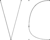
Figure 8.1 Matching derivatives of the component functions and geometric (visual) continuity are not the same: the V of VC is parametrized by two parabolic arcs with equal derivatives at the tip, but the V shape is not geometrically continuous; the C of VC is parametrized by two parabolic arcs with unequal derivatives at their common point, but the C shape is geometrically continuous.
and
Evidently, at the common point q1(1) = [00] = q2(0) the derivatives agree:
However, even with suitably cushioned end points, the V should not be handed over to boys or girls under the age of 1 for fear of injury from the sharp corner. Matching derivatives clearly do not always imply smoothness. Conversely, smoothness does not imply matching derivatives. The C of VC is parametrized by the two quadratic pieces, u,v ∈ [0,1],
and
The C is visually (and geometrically) smooth at the common point q3(1) = [00] since the two pieces have the same vertical tangent line but the derivatives do not agree:
Both examples could be made consistent with our notion of continuity for functions if we ruled out parametrizations with zero derivative and substituted v → 2v in q4. In the case of surfaces, the distinction between higher-order continuity of the component functions and actual (geometric) continuity of the surface is more subtle.
In two variables, we contrast the smoothness criteria for surfaces with the concept valid for functions by looking at two examples involving polynomial pieces in total degree B ézier form, i.e. de Casteljau’s triangles (chapter 4 on B ézier Techniques). A necessary and sufficient geometric criterion for two polynomial pieces p1, p2: R2 ![]() R/ to join C1 along a common boundary, is the ′coplanarity condition′ (chapter 4 on B ézier Techniques), illustrated in Figure 8.3,left; the function pieces p1 and p2 join C1 if all subtriangles of the control net are coplanar that share two boundary points. Since the coplanarity of the edge-adjacent triangles of the control net is a geometric criterion it is tempting to use it as a definition of smoothness for surfaces consisting of the 3-sided patches. However, the criterion is neither sufficient nor necessary.
R/ to join C1 along a common boundary, is the ′coplanarity condition′ (chapter 4 on B ézier Techniques), illustrated in Figure 8.3,left; the function pieces p1 and p2 join C1 if all subtriangles of the control net are coplanar that share two boundary points. Since the coplanarity of the edge-adjacent triangles of the control net is a geometric criterion it is tempting to use it as a definition of smoothness for surfaces consisting of the 3-sided patches. However, the criterion is neither sufficient nor necessary.
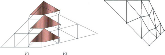
Figure 8.3 (left) Two polynomial pieces p1 and p2 join to form a C1 function if all subtriangles of the control net that share two boundary points (striped) are coplanar (Farin’s C1 condition). (right) Even though the middle cross-boundary subtriangle pair (where the patch labels p and q are placed, right) are not coplanar the two B ézier patches p(Δ) and q(Δ) join to form a tangent continuous surface.
To see that coplanarity of the edge-adjacent triangles of the control net does not imply tangent continuity of the surface consider the eight, degree 2, triangular, polynomial patches (Figure 8.2) whose control nets are obtained by chopping off the eight corners of a cube down to the midpoint of each edge. The edge midpoints and face centers of the cube serve as the control points of 8 quadratic 3-sided B ézier patches. For example, the patch in the positive octant (with thick control lines in Figure 8.2, left) has the coefficientsFigure 8.2, right shows that the patches join with a sharp crease at the middle of their common parabolic boundaries. Indeed, the normal at the midpoint  of the equatorial boundary of the positive octant patch is
  , but to match its counterpart in the lower hemisphere, by symmetry, the z-component would have to be zero. Upper and lower hemisphere therefore do not meet with a continuous normal.
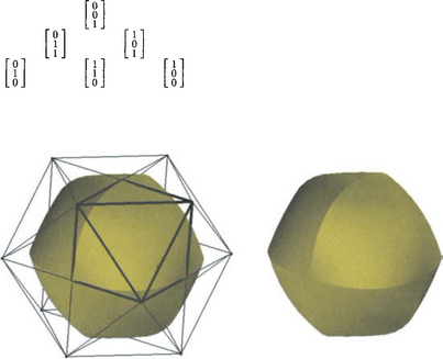
Figure 8.2 (left) The 6-point control net of one degree 2 patch in B ézier form is drawn in thick lines. The two subtriangles in the control net that include the end points of a boundary of the patch define the derivative along that boundary. For two edge-adjacent patches these subtriangles are mirror images and coplanar with their counterparts in the other patch. Still the surface defined by the patches is not tangent continuous as the creases in the surface demonstrate. (The creases are visible in the silhouette and in the change in surface shading, right).
Conversely, the geometric coplanarity criterion is not necessary for a smooth join. The two cubic pieces p, q with coefficients (c.f. Figure 8.3)
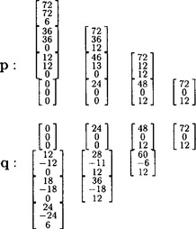
have the partial derivatives D1p = D2q along and D2p, respectively D1q across the common boundary:
With the help of Maple, we can check that the partial derivatives are coplanar at every point of the boundary, i.e. det ![]() , the zero polynomial in t. Since the surface pieces neither form a cusp nor have vanishing derivatives along the boundary, the normal direction varies continuously across (cf. Lemma 8.3.1, page 212). On the other hand, for the control point differences of the middle pair of subtriangles, labeled p and q in Figure 8.3,
, the zero polynomial in t. Since the surface pieces neither form a cusp nor have vanishing derivatives along the boundary, the normal direction varies continuously across (cf. Lemma 8.3.1, page 212). On the other hand, for the control point differences of the middle pair of subtriangles, labeled p and q in Figure 8.3,
This shows that, in contrast to a C1 match between two functions, edge-adjacent subtriangle pairs need not each be coplanar to obtain a tangent continuous surface.
8.1.1 Differentiation and evaluation
Even though derivatives of the component functions by themselves do not yield a correct picture of curve and surface continuity, the definition of geometric continuity relies on derivatives. And since we work with functions in several variables, some clarification of notation is in order.
First, it is at times clearer to denote evaluation at a point Q by f |Q rather than f(Q), evaluation on points along a curve segment E by f |E and to use the symbol o for composition, i.e. g o r = g(r). We use bold font for vector-valued functions and, somewhat inconsistently but ink-saving, regular font for directions of differentiation e and points of evaluation, say Q or 0, the zero vector in Rn. The notation Dκ for the κth derivative in one variable is consistent with the notation in two variables from [106]:
8.1.1 Definition(Differentiation)
The differentials Dκp of a map p: R2 ![]() R3 with x-, y- and z-components p[x], p[y], p[z] and the domain spanned by the unit vectors e1 ⊥ e2 are defined recursively as
R3 with x-, y- and z-components p[x], p[y], p[z] and the domain spanned by the unit vectors e1 ⊥ e2 are defined recursively as
If the Jacobian Dp is of full rank 2, p is called regular. We often abbreviate Dip = Deip.
In one variable (see e.g. [17])
This combination of the chain rule and the product rule is called Faá di Bruno’s Law and the bookkeeping is hidden in the index set

In two variables Dκ g (no subscript) is a κ-linear map acting on R2xκ (κ terms). Its component with index (i1, i2, …, ik) ∈ {1, 2}κ is Di1Di2 ˙˙˙ Diκg. The arguments of Dκg are surrounded by 〈˙〉 and 〈a, a, …, a, b, …, b〉 with a ∈ R2 repeated i times and b ∈R2 repeated j times is abbreviated as 〈(a)i, (b)j〉. We can then write the bivariate Faá di Bruno’s Law as

8.2 GEOMETRIC CONTINUITY OF PARAMETRIC CURVES AND SURFACES
This section defines k th order geometric continuity, short Gk continuity, as agreement of derivatives after suitable reparametrization, i.e. paraphrasing [58], ‘geometric continuity is a relaxation of parametrization, and not a relaxation of smoothness’. Section 3 will show that G1 and G2 are equivalent notions to continuity of the tangent and curvature(s).
8.2.1 Joining parametric curve pieces
Two Ck curve segments q: [a![]() b] → Rand p: [0
b] → Rand p: [0![]() c] → R join at p(0) with geometric continuity Gk via the Ck map ρ: R → R, ρ(0) = b, if
c] → R join at p(0) with geometric continuity Gk via the Ck map ρ: R → R, ρ(0) = b, if
The map ρ is called reparametrization. If ρ is a rigid transformation then p and g are said to join parametrically Ck and if ρ = id, the identity map, then p and g form a Ck map.
The constraint D ρ |0 > 0 rules out cusps and other singularities.
With the abbreviation  , Fáa di Bruno’s law applied to
 ![]() yields
yields
The matrix A of derivatives of ρ is called Gk connection matrix [13], [113] or β-matrix [7] and jkp is the k-jet of p. In one variable, two regular maps p and q can both be reparametrized so that p(ρp) and q(ρq) have the preferred arclength parametrization (chapter 2 on Geometric Fundamentals), i.e. unit increments in the parameter correspond to unit increments in the length of the curve. Then jk(p o ρp) |0 = jk(q o ρq) |0.
Gk splines with different connection matrices do not form a linear vector space; in particular the average of two curves that join Gk is not necessarily Gk as illustrated in Figure 8.5: if p1 and q1 join Gk via ρ1 at p1(0) and p2 and q2 join Gk via ρ2 at p2(0) = p1(0) then, in general, there does not exist a reparametrization ρ so that (1 − σ)p1 + σp2 joins Gk with (1 − σ)g1 + σg2 at p2(0) = p1(0). That is, there does not generally exist a connection matrix A such that
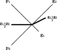
Figure 8.5 The average (bold lines) of two curves, whose pieces pi and gi join G∞, can be tangent discontinuous, i.e. its pieces do not even join G1.
In the example shown in Figure 8.5,

but  while
while  and there does not exist a G1 connection matrix
  such that
 ![]() .
.
However, if we fix a (κi + 1) × (κi + 1) connection matrix at the i th breakpoint, we can construct a space of degree k splines with prescribed Gκi joints and knots of order k - κi. Such a spline space can be analyzed as the affine image of a ‘universal spline’ whose control points are in general position [113].
Conversely, any given polygon can be interpreted as the control polygon of a Gk spline: by iterated linear interpolation (corner cutting), the polygon is refined into one whose vertices, when interpreted as B ézier coefficients, define curve pieces that join Gk, e.g. [11] for k = 2, [38] for Fr énet frame continuity (see section 8.3.1) and [113], [114], [115] for the general case.
There are degree-optimal constructions for this conversion, i.e. constructions that maximise the smoothness of the spline for a given number of corner cuts, i.e. polynomial degree. Via the notion of order of contact (see section 8.3.1) smoothness is closely related to the ability to interpolate, say the data of a previous spline segment. Following the pioneering paper [20] where it was observed that a cubic segment can often interpolate position, tangent and curvature at both end points (see also [64],[22]), Koch and Höllig [61] conjectured that, under suitable assumptions, “splines of degree ≤ n can interpolate points on a smooth curve in Rm with order of contact k − 1 = n − 1 + [(n − 1)/(m − 1)] at every nth knot. Moreover, this geometric Hermite interpolant has the optimal approximation order k + 1” (see also [101]).
8.2.2 Geometric continuity of edge-adjacent patches
We now turn to a constructive characterization of the smoothness of surfaces assembled from standard pieces used in CAGD, such as 3- or 4-sided B ézier patches, or tensor-product b-spline patches.
8.2.2 Definition(Domain, reparametrization, geometry map, patch)
• A domain is a simple, closed subset Δ of R2, bounded by a finite number of possibly curved edges Ej. Edges are not collinear where they meet.
• Let E1 be an edge of the domain Δ1 and E2 an edge of the domain Δ2. Denote an open neighborhood of a set X by N(X). Then r: N(E1) → N(E2) is a Ck reparametrization between Δ1 and Δ2 if it (1) maps E1 to E2 (2) maps points exterior to Δ1 to points interior of Δ2, and (3) is Ck continuous and invertible.
• A Ck geometry map is a map g: Δ → R3 such that Dκg, κ = 0,…, k is continuous and det(D g) ≠ 0; g(Δ) ⊂ R3 is called a Ck patch.
Regularity of the geometry map det(D g) ≠ 0, rules out geometric singularities, such as cusps or ridges, and avoids special cases – but it off-hand also rules out singular maps that generate perfectly smooth surfaces ([84], [79], [15], [102]). These constructions are shown to be smooth by a local change of variable that removes the singularity. Defining the domain boundary to consist of a few edges is specific to CAGD usage: we could have a fractal boundary separating two pieces of the same smooth surface.
The map g is called geometry map to emphasize that the local shape (but not the extent) of the surface is defined by g. The image in R3 of g restricted to its domain is the patch. The reparametrization r maps outside points to inside points to prevent the surface from folding back onto itself in a 180°-turn.
Next we join two pieces (c.f. Figure 8.6).
8.2.3 Definition(Gk join)
Two Ck geometry maps p and g join along p(E) with geometric continuity Gk via the Ck reparametrization rif
If r is a rigid transformation then p and g are said to join parametrically Ck and if r = id, the identity map, then the restrictions of p and g to their abutting domains form a Ck map.
Since p, g and r are Ck maps, Gk continuity along p(E) with Ck reparametrization r is equivalent to just k + 1 univariate polynomial equalities corresponding to differentiation in the direction e⊥ perpendicular to the edge E:
That is, as one might expect and can check by Faá di Bruno’s law, k th order continuity between two geometry maps depends on the Taylor expansion of r, p perpendicular to the edge E only up to k th order. In particular to the dege E only up to k th order. In particular, it is not necessary to know r completely.
Example Consider two C2 geometry maps p and g, and a C2 reparametrization r : r(t, 0) = (0, t). E = {(t, 0) : t ∈ [0,1]} and e⊥ = (0, − 1). An alternative reparametrization of E is {(t2, 0) : t ∈ [0,1]}. Such a definition would make the subtle point that G0 and C0 can differ as well, since the reparametrization r(t, 0) = (0, √t) is required to equate the derivatives along the boundary. (If p and g are polynomials of the same least degree then r can only be linear and p and g share the same parametrization along the edge). We write the conditions for p and g joining G2 via r along p(E) and translate them into a commonly used, abbreviated notation where guv : = D12g = De1,e2g.
In particular, for p and q defined on page 196,we compute  .
.
The example illustrates that it is convenient and shorter to give separate names, α, β, σ, τ, to the partial derivatives of r evaluated on the edge E. We can in fact specify just the partial derivatives rather than all of r: if we group the two components of each derivative into a vector we can define r in terms of Ck-j-vector fields along r(E) (Lemma 3.2 of [53]). Provided the derivatives are sufficiently differentiable in the direction e⊥ perpendicular to E we thereby prescribe the Taylor expansion of r (by the Whitney-Stein Theorem).
8.2.3 Geometric continuity at a vertex
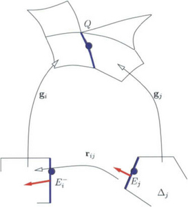
We extend our new notion of geometric continuity to n patches meeting at a common point, e.g. at a point of the global boundary where the patches may meet without necessarily enclosing the point (c.f. Figure 8.7).
8.2.4 Definition(Gk enclosure)
The Ck geometry maps gi : Δi → R3, i = 1, …, n, meet Gk via ri,i+1, i = 1, …, n − 1 with corner Q ∈ R3 if
• gi, and gi+1 join Gk via ri,i+1 along gi+1 (Ei+1),
• the normalized tangent vectors of each gi sweep out a sector of a disk and these tangent sectors lie in a common plane and may touch but do not overlap.
The Ck geometry maps form a Gk enclosure of the vertex Q if additionally gn and g1 join Gk via rn,1 along g1(E1).
The regularity of the Ck geometry maps implies that each tangent sector is the 1 to 1 image of a corner formed by the non-collinear edges E- and E of the domain. Moreover, the geometry maps do not wrap around the corner more than once. The common plane referred to above is therefore the tangent plane and, by the implicit function theorem we can expand the geometry maps as a Ck functions at Q.
Where a point is enclosed by three or more patches, additional constraints on r and g arise because patches join in a cycle. If one were to start with one patch and added one patch at a time, the last patch would have to match pairwise smoothness constraints across two of its edges. More generally, if all patches are determined simultaneously, a circular interdependence among the smoothness constraints around the vertex results. This circular dependence implies composition constraints on admissible r and vertex enclosure constraints, on the gi. The latter imply for example the important practical fact that it is not always possible to interpolate a given network of C1 curves by a smooth, regularly parametrized tangent-plane continuous surface with one polynomial patch per mesh facet [85]. A characterization, of when a curve network can be embedded into a curvature continuous surface can be found in [54].
To discuss the details, the k-jet notation (c.f. page 199) is helpful:
8.2.5 Definition
The coordinate-degree k-jet, Jkp, is a vector of directional derivatives Di1Dj2P, i, j ∈ {0,1, …, k} sorted first with key i + j, then, within each group, with key i. The total-degree k-jet, jkp, consists of the first (k2) entries of the coordinate-degree k-jet.
For example, as illustrated in Figure 8.8 (see also [59], p.61, [53]),
The composition of k-jets, jkg |r(E) ![]() jkr |E := jk(g
jkr |E := jk(g ![]() r) }E, is associative and has the identity map id as its neutral element. In k-jet notation the conditions for geometric continuity are
r) }E, is associative and has the identity map id as its neutral element. In k-jet notation the conditions for geometric continuity are
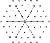
Figure 8.8 The derivative Dm1Dn2Pi of a geometry map pi at the central vertex is represented symbolically as a •, °, or ![]() placed m units into the direction of the first edge and n into the second. Elements of the total-degree 2-jet j2 are marked • elements of the coordinate-degree 2-jet J2 are marked • or °, elements of j4 are marked •, ° or
placed m units into the direction of the first edge and n into the second. Elements of the total-degree 2-jet j2 are marked • elements of the coordinate-degree 2-jet J2 are marked • or °, elements of j4 are marked •, ° or ![]() . The higher-order derivatives Hki appearing on the right hand side of the vertex-enclosure constraint system are marked by diamonds
. The higher-order derivatives Hki appearing on the right hand side of the vertex-enclosure constraint system are marked by diamonds ![]() .
.
Composition constraint on reparametrization maps: Assume now that the Ck geometry maps gi, i = 1, …, n, meet Gk via ri,i+1 with corner ![]() and
and
By the implicit function theorem, since g1 is regular, Dg1 has a left inverse in the neighborhood of 0 and that implies the Composition Constraint
i.e. the Taylor expansion up to k th order of the composition of all reparametrizations must agree with the expansion of the identity map.
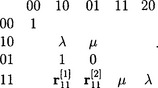
Example For k = 1 and n = 3 and with ri,j(0, t) = (t, 0) we have

With scalars λi and μi, the second equation is equivalent to the matrix product
which is in turn equivalent to
In general, the G1 constraints at 0 imply ![]() . An Expansion of the nonlinear constraints for k = 2 is shown in section 7.2 of [53].
. An Expansion of the nonlinear constraints for k = 2 is shown in section 7.2 of [53].
8.2.1 Lemma
A symmetric reparametrization rij = r that satisfies the Composition Constraint for a given n is defined by
Proof The eigenvalues of Dr are the n th unit roots ![]() Therefore
Therefore ![]() Since, by Fáa di Bruno’s law, at least one factor of the expansion of
Since, by Fáa di Bruno’s law, at least one factor of the expansion of ![]() is a higher derivative of r,
is a higher derivative of r, ![]()
Vertex enclosure constraints: Another set of constraints applies to geometry maps. Since the Gk constraints of two edge-adjacent patches have support on the first k layers of derivatives counting from each edge, the constraints across two consecutive edges of a geometry map share as variables the derivatives Dm1Dn2 with m ≤ k and n ≤ k at the vertex, i.e. overlap on the coordinate-degree k-jet of the geometry map at the vertex (markers • and ° in Figure 8.8).
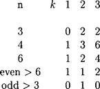
If n is the number of patches surrounding the vertex, then there are n(k:+l)2 overlapping continuity constraints and an equal number of variables in the form of derivatives in the corresponding coordinate degree k-jets Jkpi. Can the constraints can always be enforced by choosing Jkpi appropriately? Already for k = 1, the resulting 4n by 4n constraint matrix M is not invertible if n is even but it is invertible for n odd. For k > 1, more complex rank-deficiences arise while the right hand side is in general not in the span of the constraint matrix: unlike the univariate case, where we consider only the first k derivatives for Gk joins, the Gk vertex-enclosure constraints involve derivatives of up to order 2k!
Depending on the data and the construction scheme, some of the higher derivatives are fixed. For example, prescribing boundary curves pins down Di1D02p for all i. Even when the goal is to just identify degrees of freedom of a free-form spline space [37],[65], the underlying splines must have consistent derivatives up to order 2k. There is one well-studied exceptional case: if the corner Q is the intersection of two regular Ck curves and n = 4 then the constraint system becomes homogeneous, removing the linkage between the k-jets and the higher derivatives. Since the constraint matrix is additionally rank deficient it is possible to interpolate the curve data by low-degree, parametrically Ck surfaces [40],[41]. The corresponding free-form splines are tensor-product splines in the sense of Coons and Gordon [18],[41].
When the reparametrizations are linear as in Lemma 8.2.1 then determining the matrix rank is similar to determining the dimension of a spline space [2], however with the additional requirement that the ‘minimal determining set’ Dm1Dn2pi be symmetric. By contrast, the analysis of the dimension of spline spaces allows choosing one geometry map completely and then finding extensions that respect the continuity constraints. This misses the crucial rank deficiencies that depend on the parity of k and n.
Vertex-enclosure constraints are weaker than compatibility constraints. For example, the twist compatibility constraint requires that mixed derivatives are prescribed consistently since D1D2p = D2D1p must hold for a polynomial finite element (see e.g. [4]). Mixed derivatives at a vertex can be prescribed inconsistently by independently prescribing transversal derivatives along abutting edges emanating from the vertex.
Incompatibility can be accomodated by using poles or singular parametrizations (see page 8.4,(2), 3rd and 4th item).
The main task ahead is to characterize the rank deficiencies of the n(k +1)2 x n(k + 1)2 matrix M of the Gk constraint system
in the variables Dm1Dn2pi |0, n, m ∈ {0, …, k}, i = 1, …, n. In terms of k-jets and Hki := (Dk+m1 Dl2pi)m=1, …,k,l=0, …,k-m, the vector of higher derivatives of pi, for example, H2i := (D31pi, D31D2pi, D41pi), the constraint system reads (all blank entries are zero)
As for connection matrices in the univariate case, page 199, the entries of each (k + 1)2 x (k + 1)2 matrix Mi and each (k + 1)2 x k(k + l)/2 matrix Ni are derivatives of ri. Mt,i corresponds to the (k + 2)(k +1)/2 homogeneous constraints jkpi−1 = Mt,ijkpi that involve only derivatives of total degree k or less (• in Figures 8.8 and 8.9) and that can always be enforced by choosing one of the jets, say jkp1, and extending it to the remaining patches; that is, the total-degree k-jets represent a single polynomial expansion up to total degree k at the vertex, a characterization that is also known as the n + 1–Tangent Theorem [81], [56].
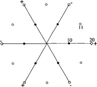
Figure 8.9 The total-degree 1-jet, illustrated as ‘•’, represents the same linear function for all patches. The n = 6 constraints involving the ‘11’ derivatives D11D12, °, in the coordinate-degree 1-jet but not the total-degree 1-jet give rise to a 6 × 6 matrix Mc that is rank deficient by 1, i.e. of rank 5. This (vertex-enclosure) constraint can only be solved if the right hand side, defined by the (component normal to the tangent plane of the) ‘20’ derivatives D21D02, ![]() , lies in the span of the constraint matrix. If all reparametrizations are the same, this is the case exactly when the alternating sum of the ‘20’ derivatives is zero, i.e. if the average of the elements marked + equals the average of the elements marked –.
, lies in the span of the constraint matrix. If all reparametrizations are the same, this is the case exactly when the alternating sum of the ‘20’ derivatives is zero, i.e. if the average of the elements marked + equals the average of the elements marked –.
Each submatrix Mc,i corresponds to the remaining k(k + 1)/2 constraints that involve derivatives of total degree greater than k (the diamonds ![]() in Figure 8.8 and 8.9). By blockwise elimination, the rank deficiency of M equals the rank deficiency of I - Π Mi and the solvability for arbitrary right hand side depends, after removal of the homogeneous constraints, only on the rank of I - Π Mc,i. Each submatrix Mc,i decomposes further into skew upper triangular matrices Mk,
in Figure 8.8 and 8.9). By blockwise elimination, the rank deficiency of M equals the rank deficiency of I - Π Mi and the solvability for arbitrary right hand side depends, after removal of the homogeneous constraints, only on the rank of I - Π Mc,i. Each submatrix Mc,i decomposes further into skew upper triangular matrices Mk,![]() ,i of size
,i of size ![]() ×
× ![]() that are grouped along the diagonal.
that are grouped along the diagonal.
Example For k = 1 we have the constraints at 0 (c.f. Figure 8.9) and rab := Da1Db2r |0
That is, dropping the subscript i for simplicity, each matrix-block [MN] of G1 constraints has the form
Here N is the last column, below ‘20’. The entries mn to the left of the matrix indicate that the row corresponds to the constraint Dm1 Dn2(pi−1 - (pi ![]() ri)) = 0 while the entries on top indicate the derivatives Dm1 Dn2pi that enter the constraint as variables. For example, the column ‘20’ corresponds to the variable D21pi. The constraint rows labeled ‘00’,‘01’, and ‘10’ correspond to the total-degree 1-jet and are solvable leaving j1P1 free to determine the tangent plane by its three variables D01 D02p1 |0 = p1(0), D1p1(0) |0 = P1(0), D1p1(0) and D2P1(0) with normal n = D1p1(0) Λ D2P1(0). The (more interesting) constraint matrix Mc corresponds to the constraint row and column ‘11’. With p11i = n ˙ D11D12pi and p20i = n ˙ D21pi
ri)) = 0 while the entries on top indicate the derivatives Dm1 Dn2pi that enter the constraint as variables. For example, the column ‘20’ corresponds to the variable D21pi. The constraint rows labeled ‘00’,‘01’, and ‘10’ correspond to the total-degree 1-jet and are solvable leaving j1P1 free to determine the tangent plane by its three variables D01 D02p1 |0 = p1(0), D1p1(0) |0 = P1(0), D1p1(0) and D2P1(0) with normal n = D1p1(0) Λ D2P1(0). The (more interesting) constraint matrix Mc corresponds to the constraint row and column ‘11’. With p11i = n ˙ D11D12pi and p20i = n ˙ D21pi
By the Composition Constraint on page 205, Πni=1 μi = (−1)n. Therefore the rank of the matrix is n − 1 if n is even and n if n is odd [111], [112], [28], [128], [84], [29]. Moreover, if we assume symmetry, i.e. μi = −1 and λi = λ for i = 1, …, n, and if n is even then the vector v with v(i) = (−1)i spans the null space of Mc and therefore the Alternating Sum Constraint has to hold for the system to be solvable (c.f. Figure 8.9): if λ≠ 0 then

where
[MN] decomposes into the upper left 6×6 block Mt and, from columns ‘21’, ‘12’ and ‘22’,
Remark: C, J and K above depend directly on D and E in the C2 reparametrization matrix. To define a weaker notion of continuity in the spirit of Fr énet-frame continuity for curves of section 8.3.1 one would choose C, J and K independently.
For the remainder of the discussion we assume that all rij are linear and equal to r, as in Lemma 8.2.1 (see [86] for a more general analysis and [30] and [126] for a discussion of the case k = 2 in terms of B ézier coefficients). Such equal reparametrization is the natural choice for filling ‘n-sided holes’ (Chapter N-sided Patches), and does not force symmetry of the patches: the tangent vectors, for example, need not span a regular n-gon (but span the affine image of a regular n-gon). If n = 4 then rank(I - (Mk,![]() )n) = 0. That is, in the tensor-product case, since Nc = 0, one full coordinate-jet Jkp1 can be chosen freely and Jkp2, Jkp3 and Jkp4 are determined uniquely by the continuity constraints. For general n, the rank deficiencies of I - Mnc for k = 1, 2, 3 are listed in the following table. The results for larger k are sumarized in a conjecture in [86].
)n) = 0. That is, in the tensor-product case, since Nc = 0, one full coordinate-jet Jkp1 can be chosen freely and Jkp2, Jkp3 and Jkp4 are determined uniquely by the continuity constraints. For general n, the rank deficiencies of I - Mnc for k = 1, 2, 3 are listed in the following table. The results for larger k are sumarized in a conjecture in [86].
Since only the Taylor expansion is of interest, the vertex enclosure constraints are independent of the particular representation of the surrounding geometry maps. In particular, the vertex enclosure constraints apply to rational geometry maps in the same fashion as to polynomial geometry maps unless the denominator vanishes. The four known techniques for enforcing the vertex-enclosure constraints are listed in section 8.4, page 218.
8.2.4 Free-form surface splines
One interpretation of the two types of maps defining the Gk free-form surface spline is that the reparametrizations r define, by gluing together domains, an abstract manifold whose concrete immersion into R3 is defined by the geometry maps, e.g. Figure 8.10. Free-form surface splines have a bivariate control net with possibly n-sided facets and m-valent nodes. Alternative names are G-splines [62] and geometric continuous patch complexes [53]. Geometric continuous patch complexes differ in their characterization by requiring additionally a connecting relation that identifies (glues together) domain edges [53], [50], [104], This connecting relation is needed when Gk continuity is defined in terms of the existence of reparametrizations rather than by explicitly identifying the (first k + 1 Taylor terms of the) reparametrization.
8.2.6 Definition
A Gk free-form surface spline is a collection of Ck geometry maps and reparametrizations such that
• at most one reparametrization is associated with any domain edge;
• if a reparametrization rij exists between the edge E of the domain Δi of gi and an edge of the domain of gj then gi and gj join with geometric continuity Gk via rij along gi(E) and rij is Ck;
• any sequence of Ck geometry maps gi : Δi→ R3, i = 1, …, n, such that gi and gi+1 join Gk via ri,i+1 along gi+1(Ei+1), and gi(Ei(0)) = Q, meet Gk with corner Q ∈ R3.
Free-form surface splines with different reparametrizations do not form a linear vector space. This follows directly from the same statement for Gk continuous curves. For example, we can replace lines with planes in the example shown in Figure 8.5. However, if all reparametrizations agree then we can form an average free-form surface spline and the average inherits the continuity by linearity of differentiation. section 8.4 outlines constructions.
8.3 EQUIVALENT AND ALTERNATIVE DEFINITIONS
8.3.1 Matching intrinsic curve properties
In [13], Boehm argues that there are (only) two types of geometric continuity: contact of order k, a notion equivalent to Gk continuity, and, secondly, continuity of geometric invariants (but not necessarily of their derivatives).
Two abutting curve segments have contact of order k if they are the respective limit of two curve sequences whose corresponding elements intersect in k + 1 points and these points coalesce in the limit. In particular, for a space curve x : R → R3 with Fr énet frame (chapter 2 on Geometric Fundamentals) spanned by the tangent vector t, the normal vector m and the binormal b and ′ denoting the derivative with respect to arc length
contact of order 2 implies that x′ = t and x ′ are continuous and therefore that tangent, normal and curvature are continuous. Contact of order 3 implies continuity of x ′, x ′ and x ′′ and therefore continuity of Fr énet frame, curvature and torsion. Moreover, the derivative of the curvature must be continuous tying the entry labeled α in the connection matrix displayed on page 199 in section 8.2.1 to quantities already listed in the matrix. Similarly, contact of order k in R3 requires k ∈ Ck−2 and τ ∈ Ck−3 and therefore further dependencies among the entries [42].
By contrast, continuity of the k th geometric invariant, also called kth order Fr énet frame continuity [31], [38], and abbreviated Fk, does not require that the α-entry (or, more generally, any subdiagonal entry) depend on other entries in the connection matrix. Fr énet frame continuity requires that the frame of the two curve pieces agrees and only makes sense in Rd, for d ≥ k. Boehm [13] shows that while geometric continuity is projectively invariant, Fr énet frame continuity is not. For surfaces, an analogous notion of continuity in terms of fewer restrictions on the connection matrix entries, is pointed out on page 209.
8.3.2 Ck manifolds
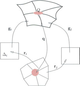
Differential geometry has a well-established notion of continuity for a point set: to verify k th order continuity, we must find, for every point Q in the point set, an invertible Ck map (chart) that maps an open surface-neighborhood of Q into an open set in R2. If two surface-neighborhoods, with charts q1 and q2 respectively, overlap then q2![]() q−11 : R2 → R2 must be a Ck function. This notion of continuity is not constructive: while it defines when a point set can be given the structure of a Ck manifold, say a Ck surface, it neither provides tools to build a Ck surface nor a mechanism suitable for verification by computer.
q−11 : R2 → R2 must be a Ck function. This notion of continuity is not constructive: while it defines when a point set can be given the structure of a Ck manifold, say a Ck surface, it neither provides tools to build a Ck surface nor a mechanism suitable for verification by computer.
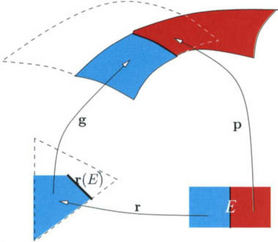
However, geometric continuity and the continuity of manifolds are closely related: every point in the union of the patches of a Gk free-form surface spline admits local parametrization by Ck charts if the surface does not self-intersect: the union is an immersed Ck surface with piecewise Ck boundary. We face two types of obstacles in establishing this fact. First, the geometry maps should not have geometric singularities on their respective domains since these would prevent invertibility of the charts, and the spline should not self-intersect so that we can map a neighborhood of the point in R3 to the plane in a 1−1 fashion. Establishing regularity and non-self-intersection requires potentially expensive intersection testing (chapter 25 on Intersection Problems). The second apparent obstacle is that the patches that make up the surface are closed sets that join without overlap. Therefore the geometry maps cannot directly be used as charts. However, as illustrated in Figure 8.11, we can think of the charts as piecewise maps composed of n maps qi = r−1i ![]() g−1i that map open neighborhoods in R3 (grey oval) to open neighborhoods in R2 (grey disk). The constructions [50],[78],[19] explicitly start by constructing the union of neighborhoods and connecting charts and then compose these with (rational) spline basis functions.
g−1i that map open neighborhoods in R3 (grey oval) to open neighborhoods in R2 (grey disk). The constructions [50],[78],[19] explicitly start by constructing the union of neighborhoods and connecting charts and then compose these with (rational) spline basis functions.
8.3.3 Tangent and normal continuity
A number of alternative characterizations exist to test a given G1 free-form spline complex for tangent continuity or to derive G1 free-form splines. The criteria consist of an equality constraint establishing coplanarity of the first partial derivatives at each point of the common boundary of two patches (c.f. Figure 8.4), and an inequality constraint on the reparametrization that prevents a 180°-flip of the normal for the regular geometry maps. In the following lemma, e is the direction along the preimage E of the common boundary p(E) and, as is appropriate for least degree polynomial representations (see page 202), p and g have the same parametrization along p(E).
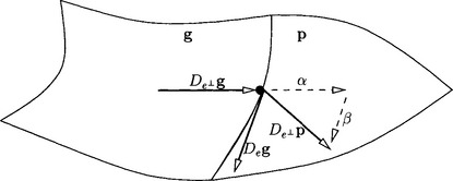
Figure 8.4 If the patches meet with tangent continuity, the transversal derivative De⊥p of p must be a linear combination of the versal derivative vector De g in the direction e along the preimage E of common boundary p(E) and the transversal derivative De⊥g in the direction e ⊥ perpendicular to e: De⊥p = αDeg + βDe⊥g.
8.3.1 Lemma(Tangent continuity)
Let p and g be regular parametrizations and p |E = g |E. The maps λ, μ and v are univariate scalar-valued functions and
are functions restricted to an edge E mapping into R3. The following characterizationsof G1 continuity are equivalent.

With ![]() , (2) is the definition of a G1 join in Definition 8.2.3. Figure 8.4 illustrates the geometric meaning of (2).
, (2) is the definition of a G1 join in Definition 8.2.3. Figure 8.4 illustrates the geometric meaning of (2).
Proof Regularity implies n(t) ≠ 0 for all t on E.
(1) ⇒ (2): Adding the two equalities (Ie) after multiplication with v = −αg and μ = αp respectively (2e) holds in the form ![]() .
.
(2) ⇒ (3): The inner product of both sides of (2e) with n yields (3e). The cross product ∧ of (2e) with c followed by the inner product ˙ with μn yields ![]() . Then (2i) implies (3i).
. Then (2i) implies (3i).
(3) ⇒ (4): From (3e) we have n ⊥ De⊥p and, by definition, n ⊥ c. By regularity ![]() and (3i) decides the sign.
and (3i) decides the sign.
(4) ⇒ (1): Regularity and (4) imply (1e) that the partial derivatives De⊥ p and De⊥ g can be expressed in the same (orthogonal) coordinate system-spanned by t and c. The cross product of each equality with c yields ![]() and by sign comparison (1i).
and by sign comparison (1i).
Formulation (4), comparison of normals, can be turned into a practical tool for quantifying tangent discontinuity. While (1), (2) and (3) are unique only up to scaling, and therefore ∈-discontinuity′ measured as ![]() or
or ![]() or
or ![]() is not well-defined, the angle between the two normals is scale-invariant.
is not well-defined, the angle between the two normals is scale-invariant.
The symmetric characterization (1) asserts the existence of a Taylor expansion along the boundary that is matched by g and p. This has been used for constructions [16], [83], [105]. The direct equivalence of (1) and (2) for polynomials is proven in [23] and [55] generalizes this Taylor-expansion approach to k th order.
If p and g are rational maps, i.e. quotients of polynomials, the continuity conditions can be discussed in terms of polynomials in homogeneous coordinates keeping in mind that we may scale freely by a scalar-valued function σ(u,v): Dkp |E = Dk(σ g ° r) |E, k = 0, …,k [127].
If p and g are polynomials then, up to a common factor, so are the scalar functions, λ, μ and v in (1). In fact, after removal of common factors, the degree of the functions is bounded by the degree of p and g. This comes in handy when looking for possible reparametrizations r between two geometry maps.
8.3.2 Lemma
If p and g are polynomials, then, up to a common factor, λ, μ and v in (1) are polynomials of degree no larger than respectively
Proof Due to regularity of g along the boundary, the pre-image of the boundary is covered by overlapping intervals U such that for each U there are two components i, j ∈ {x, y, z} with det  g[j] the j th component of g. Therefore we can apply Cramer’s rule to
and obtain
The degree of λ, μ and v is bounded by the degrees of the determinants since the common factor v/ det Mij can be eliminated in the constraints. Since det Mij vanishes at most at isolated points, the degree bound can be extended from U to the whole interval.
The characterizations of geometric continuity in terms of geometric invariants (tangents, curvatures) are characterizations of continuity by covariant derivatives [53].
8.3.3 Lemma
Two Ck geometry maps p and g join with geometric continuity Gk via the Ck reparametrization r along p(E) if there exist normal vector fields np and ng of p and g respectively such that
In particular, Dn represents the shape operator [68], principal curvatures and directions [120], [58] or the Dupin indicatrix [67]. [58] shows in particular equivalence of G2 continuity with curvature continuity based on sharing surface normal, principal curvatures and principle curvature directions in R3.
8.3.4 Global and regional reparametrization
Often we can view a free-form surface as a function over a domain with the same topological genus, e.g. an isosurface of the electric field surronding the earth may be computed as a function over a sphere [1], More generally, we can assemble an object of the appropriate topological genus by identifying edges of a planar domain and then define a standard spline space over the planar domain, mapping into R3 with additional periodic boundary conditions and creating ‘orbifolds’ [35], [123]. This approach circumvents the need for relating many individual domains via reparametrizations, since there is only one global domain (modulo periodicity). Basis functions with local support in the domain yield local control. For practical use one has to consider three points. First, the genus of the object has to be fixed before the detailed design process can begin - so one cannot smoothly attach an additional handle later on. Second, the spline functions have to be placed with a density that anticipates for example, an ornate protrusion of the surface where more detail control is required. Third, the ‘hairy ball theorem’, the hair on a tennis ball cannot be smoothly combed down without leaving a bald spot or making a parting, implies that the global mapping from subsets of the plane to, say, the sphere has a singularity. The theorem, a consequence of the Borsuk-Ulam theorem, states more formally “If f : S2 → S2 is a continuous map from the sphere to itself then there exists a point where x and f(x) are not orthogonal as vectors in R3” and in particular, with x a point on the sphere S2 and f(x) a corresponding unit tangent, “the tangent field on a sphere in R3 has to have a singularity”. The singularity is nicely illustrated in [57].
Prautzsch [99], and co-workers [76],[100], and Reif [102], [104] developed the idea of filling n-sided holes by building a regional parametrization r for a neighborhood of a point Q where n patches meet (see Figure 8.13). The regional parametrization stands in contrast to the local reparametrizations along an edge used to define free-form surface splines, and the global parametrization discussed earlier. The regional parametrization is composed with a single map g, for example a quadratic polynomial. This approach considerably simplifies reasoning about the resulting surfaces. By separating issues of geometric shape from valence and local topology, verification of smoothness of the resulting surfaces at Q (which could be a major effort of symbolic computing) reduces to showing that r is smooth since smoothness is preserved under composition with an (infinitely smooth) polynomial geometry map. Reparametrization gives g ° r the structure of a collection of standard (tensor-product or total-degree) patches that can then be connected to a surrounding ring of spline patches p via Hermite interpolation H(p, g ° r) of degree (degree of g times degree of r). By fixing the degree d of the polynomial beforehand, independent of the smoothness k to be achieved, and choosing the Ck parametrization in the domain to be of bidegree (k + 1), the regional schemes were the first to claim a construction of Ck surfaces of a degree linear in k, namely of degree d(k + 1). In particular, Prautzsch and Reif proposed to choose polynomials of degree d = 2 which yields G2 free-form constructions of degree bi-6.
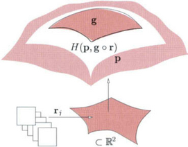
Figure 8.13 Regional parametrization: an n-sided cap g is Hermite-extended via H(p, g° r) to match a given spline complex p.
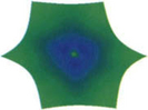
Fixing the degree of g comes at a cost. While quadratics come in a large number of shapes [93] they are not able to model, for example, higher-order saddle points. A higher-order saddle point is a point on a C2 surface with three or more extremal curvature directions; hence it has zero curvature as illustrated in Figure 8.14. Since quadratics that have a point of zero curvature must be linear this yields flat patches rather than a flat point. For the particular example of a 3-fold saddle point, we could address this shortcoming by increasing the degree of the polynomial to three and the overall degree to bi-9 [104]. But this does not address the underlying problem, namely the mismatch between n patches meeting at Q and the fixed number of coefficients of any single polynomial of fixed degree d. In [89] it was therefore suggested to replace g by a (total-degree cubic) spline. This yields at least n degrees of freedom.
8.3.5 Implicit representation
Under suitable monotonicity and regularity constraints the zero set of a trivariate polynomials in BB-form over a unit simplex defines a single-sheeted, singly connected piece of surface that we can also call a patch (chapter 15 on Algebraic Methods). If p,q : R3 → R are two trivariate polynomials in BB-form that join Ck functions at a common point E ∈ R3 or across a common curve E ∈ R3 then generically (see caveat below) the corresponding patches join with contact of order k at E:. E is the limit of k + 1 intersection points (curves) Ej of functions pj and qj converging respectively Ej → E, Pj → p and qj → q. Just as in the parametric case, we have to make sure that the trivariate polynomials are regular at E, as the following example demonstrates: Let p(x, y, z) = x2 + y3, x ≤ 0, q(x,y, z) = x2 + y3, x ≥ 0. Both p and q are polynomial pieces, have single-sheeted, singly connected zero sets and join Ck for any k; but the zero set is not smooth at the intersection (see Figure 8.15 left for a cross-section.)
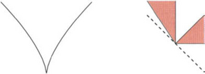
Figure 8.15 (left) Zero set of x2 + y3 = 0 and (right) tangent sectors of two possibly smooth patches whose relative position does not allow the reduction to smoothness of a curve by cutting with a transversal plane (dashed line).
Since we are only concerned with the zero set of the polynomial, we do not actually need that the polynomials join smoothly but can scale the joining pieces by scalar functions a and b ([125], [124], [72]):
8.3.1 Definition
Two trivariate polynomials p and q join with Gk continuity at Q if
Two trivariate polynomials p and q join with Gk continuity along an irreducible curve
One could intersect E with a transversal plane to obtain curves meeting in a point and avoid a separate definition for continuity along E (The analogous technique for parametric surfaces is called Linkage Curve Theorem [81], [56].) This approach, however, runs into technical problems, since implicit patches have corners and there may be just one point of intersection with a transversal plane. Similarly, the trivariate k-jet jkp cannot just be replaced by a k-jet along a line [36] since the domains may lie in the same half space and thus there is no plane that intersects both restricted domains in more than the common point (see Figure 8.15, right.)
8.3.6 Generalized subdivision
Near n-valent mesh nodes, uniform generalized subdivision surfaces consist of an infinite sequence of ever smaller, concentric rings that are internally parametrically Ck. The rings also join one another parametrically Ck. Yet, by the Borsuk-Ulam theorem (section 8.3.4) there cannot be a parametrically Ck mapping from the plane to objects of arbitrary genus without a singularity. In a sense the (effect of the) necessary reparametrization is therefore concentrated near the limit points of n-valent mesh nodes. Correspondingly, the analysis of smoothness of generalized subdivision surfaces has focused on the limits of the n-valent mesh nodes (see e.g. [3] [94], [95]). At present it appears that uniform generalized subdivision cannot generate curvature continuous surfaces unless the control net is in special position.
8.4 CONSTRUCTIONS
An algorithm for constructing Ck surfaces subject to data, such as a control net or a prescribed network of curves, is a specification of the Ck reparametrizations r up to k th order and of the geometry maps g (see also n-sided hole filling (Chapter N-sided Patches)).
The generic approach of stitching together individual spline patches (after possibly manipulation or refinement of the control structure) consists of
• choosing a consistent reparametrization r at the n-valent points and deriving a reparametrization for two edge-ajacent patches as a Hermite interpolant to the reparametrizations at the end points of the edge;
• solving the vertex-enclosure problem at each point and deriving the geometry maps of abbutting patches as a Hermite interpolant to the Taylor expansions at the vertices.
The generic construction is as follows.
(1) If n0 patches join at one boundary endpoint, corresponding to s = 0, t = 0, and n1 patches join the other with s = 1, t = 0 then a Hermite interpolant (in s) to the linear symmetric reparametrization of Lemma 8.2.1 at the endpoints, up to k th order is given by
where α(s) and β(s) are Ck functions such that α(s), β(s) ≥ 0,
The interpolant is constructed so that the Taylor expansions of the reparametrization at either endpoint do not interfere, i.e. Dk2r(i) = 0 for i ∈ {0,1}, k > 1 [47], For the special, tensor-product transition case of n1 = 4, we obtain the ‘Tannenbaum’ layout of B ézier coefficients shown in Figure 8.16.
Figure 8.16 Generic ‘Tannenbaum’ layout of B ézier coefficients along a boundary (horizontal line) between two patches that transition from a 4-valent point (left) to an n-valent point (right).
(2) The vertex-enclosure problem (for example for G1, n even) can be solved by one the following four techniques [84]:
1. Choosing Hki (e.g. the curve mesh) in the span of the constraint matrix M;
2. Splitting patches whose boundaries are prescribed into two or more pieces so that the boundary curves of the split patches can be freely chosen in the span of the constraint matrix (e.g. [32], [33], [96]);
3. Using rational patches to introduce second-order poles at the vertices (e.g. [43], [16] [54]);
Thus, if we are not concerned about the degree, it is straightforward to create Gk freeform surface splines for any k. The focus over the past decade has been to reduce the degree of the surface representation, and to obtain better surface shapes (Chapter on Surface Fairing). For example, while the degree of curvature continuous surfaces prior to [99] and [102] was at least bi-9 (100 coefficients per patch) [131], [52] newest results achieve curvature continuity with at most 24 coefficients per patch [90].
Some special techniques, in particular for tangent continuity (c.f. Lemma 8.3.1), are as follows.
• Given the common boundary with derivative c = Dep |E = Deg |E, [16], [83], [23] use a symmetric construction, picking t as minimal Hermite interpolant to the transversal derivative data at the endpoints and
with t ∧ c ≠ 0 and αp ≠ 0 ≠ αg, cf. Lemma 8.3.1.
• As illustrated in Figure 8.5 the average of two G1 joined curves or surfaces is generally not G1. But if all transversal derivatives of a patch along a boundary E(t) are collinear with a vector v, i.e.
for scalar functions p and q with q/p < 0 then n = N/||N || where N(t) := Dep |EΛv is a normal common to both patches along the boundary [103].
• Sabin [109] and [82] use formulation (2) of Lemma 8.3.1, n Λ Dp = 0, to determine versal and transversal derivatives of p, for given n - thereby isolating the construction of a patch from its neighbor.
• [73] and [83] list a number of choices for reparametrizations for particular constructions.
8.4.1 Free-form surface splines of low degree
Goodman [37] introduced G1 splines of degree bi-2 for special control meshes that consist of quadrilateral facets and vertices of valence 3 or 4. The prototype meshes, that can be modified by quadrilateral refinement, the cube mesh and the dual of the cube with lopped off corners, are sphere-like shapes that, when symmetric, are curvature continuous (see [92]). Splitting each original quadrilateral facet 1 to 4, [103] derives a bi-2 G1 free-form surface spline. Splitting each quadrilateral facet into four triangles, [88] obtains a G1 construction of total degree 3 that also satisfies the local convex hull property, i.e. the surface points are guaranteed to be an average of the local control mesh. All constructions with quadratic boundary curve, however, suffer from a slight shape defect when they are to model a higher-order saddle point : due to the Alternating Sum Constraint on page 8.2.3 the quadratic boundary curves must lie on a straight line. If the construction is additionally based on tensor-product patches then the shape defect is very noticable [49],[91] at higher-order saddle points.
The Gk free-form spline constructions of Prautzsch [99] and Reif [102] are of degree 2(k + l) if flat regions at higher-order saddle points are acceptable – and of degree d(k + 1) if modeling of the local geometry requires a polynomial of degree d. [49] shows that a G2 degree bi-5 construction is possible; as stated the construction has a shape defect due to the quadratic boundary curve. At least algebraically, we can now model C2 free-form surfaces of unrestricted patch layout from patches of maximal degree (d + 2, 3), d > 0 with the flexibility of degree d, C2 splines at extraordinary points [90]. This approach generalizes to Ck surfaces of piecewise bidegree k + 1, 2k + d − 2.
8.5 ADDITIONAL LITERATURE
Every paper on smooth surfacing defines some, possibly specialized, notion of geometric continuity. Some of the early characterizations can be found in [10] [9], [8] [24] [28] [32] [34] [70] [73] [75] [80] [108],[107] [110], [111], [112], [118], [116], [117], [46],[85], [96], [121], [119] [120] [130] [120] [129] and characterizations for curves in [6], [7], [51], [21], [31].
A number of publications specifically aim at clarifying the notion of geometric continuity. Kahmann discusses curvature and the chain rule [67], DeRose [24] reconciles continuity after reparametrization with the smoothness of manifolds (see also [26], [27]). Liu [74]characterizes G1 constraints in the form (1) of Lemma 8.3.1. Particularly well-illustrated is Boehm’s treatment of geometric and ′visual′ continuity [11], [12] [14], [13]. Herron [58] shows directly the equivalence of first and second order geometric continuity with tangent and curvature continuity of surfaces. Further characterizations can be found in [63], [98],[97], [23], [55], [25], [126], [122].
Hahn’s treatment of geometric continuity [53] (see also [42]) served as a blueprint for section 8.2 but differs in that he defines a Gk join in terms of the existence of a reparametrization, rather than making the reparametrization part of the definition.
Warren’s thesis [125] looks at geometric continuity of implicit representations and [36] is a tour de force of conversions of notions of geometric continuity between two patches.
I am indebted to Tamas Hermann for closely reading the article and making numerous suggestions. Kestas Karicauskas introduced me to the term ‘Tannenbaum’ configuration (Christmas tree configuration).
1. Alfeld, P., Neamtu, M., Schumaker, L.L. Bernstein-Bézier polynomials on spheres and sphere-like surfaces. Computer Aided Geometric Design. 1996;13(4):333–349.
2. July Alfeld, P., Schumaker, L.L. On the dimension of bivariate spline spaces of smoothness r and degree d = 3r + 1. Numerische Mathematik. 1990;57(6/7):651–661.
3. Ball, A.A., Storry, D.J.T. Conditions for tangent plane continuity over recursiveley generated B-spline surfaces. ACM Transactions on Graphics. 1988;7(2):83–102.
4. Barnhill, R., Gregory, J. Compatible smooth interpolation in triangles. J of Approx. Theory. 1975;15(3):214–225.
5. Barry, P.J., Dyn, N., Goldman, R.N., Micchelli, C.A. Identities for piecewise polynomial spaces determined by connection matrices. Aequationes Math. 1991;42(2–3):123–136.
6. December Barsky, B.A. The Beta-spline: A Local Representation Based on Shape Parameters and Fundamental Geometric Measures. PhD thesis, University of Utah. 1981.
7. November Barsky, B.A., DeRose, T.D. Geometric continuity of parametric curves: Three equivalent characterizations. IEEE Computer Graphics and Applications. 1989;9(6):60–69.
8. May Beeker, E. Smoothing of shapes designed with free-form surfaces. Computer-Aided Design. 1986;18(4):224–232.
9. translated by R. Forrest Bézier, P. Numerical Control: Mathematics and Applications. Wiley; 1972.
10. February Bézier, P. Essai de definition numerique des courbes et des surfaces experiment ales. PhD thesis, Universite Pierre et Marie Curie. 1977.
11. March Boehm, W. Curvature continuous curves and surfaces. Computer-Aided Design. 1986;18(2):105–106.
12. Boehm, W. Smooth curves and surfaces. In: Farin G., ed. Geometric Modeling: Algorithms and New Trends. SIAM; 1987:175–184.
13. Letter to the Editor Boehm, W. On the definition of geometric continuity. Computer-Aided Design. 1988;20(7):370–372.
14. Boehm, W. Visual continuity. Computer-Aided Design. 1988;20(6):307–311.
15. Bohl, H., Reif, U. Degenerate Bézier patches with continuous curvature. Computer Aided Geometric Design. 1997;14(8):749–761.
16. (3) Chiyokura, H., Kimura, F., Design of solids with free-form surfaces [July] Computer Graphics (SIGGRAPH ’83 Proceedings). 1983:289–298.
17. Constantine, G.M., Savits, T.H. A multivariate Faà di Bruno formula with applications. Trans. Amer. Math. Soc. 1996;348(2):503–520.
18. June Coons, S.A. Surfaces for computer-aided design of space forms. Technical Report MIT/LCS/TR-41, Massachusetts Institute of Technology. 1967.
19. Navau, J.C., Garcia, N.P. Modelling surfaces from planar irregular meshes. Computer Aided Geometric Design. 2000;17(1):1–15.
20. December de Boor, C., Höllig, K., Sabin, M. High accuracy geometric hermite interpolation. Computer Aided Geometric Design. 1987;4(4):269–278.
21. August Degen, W.L.F. Some remarks on Bézier curves. Computer Aided Geometric Design. 1988;5(3):259–268.
22. August Degen, W.L.F. High accurate rational approximation of parametric curves. Computer Aided Geometric Design. 1993;10(3):293–314.
23. June Degen, W.L.F. Explicit continuity conditions for adjacent Bézier surface patches. Computer Aided Geometric Design. 1990;7(1–4):181–189.
24. DeRose, T. Geometric Continuity: A Parametrization Independent Measure of Continuity for Computer Aided Design. PhD thesis, UC Berkeley, California. 1985.
25. June DeRose, T.D. Necessary and sufficient conditions for tangent plane continuity of Bézier surfaces. Computer Aided Geometric Design. 1990;7(1–4):65–179.
26. DeRose, T.D., Barsky, B.A. An intuitive approach to geometric continuity for parametric curves and surfaces. In: Wein M., Kidd E.M., eds. Graphics Interface ’85 Proceedings. Philadelphia: Canadian Inf. Process. Soc.; 1985:343–351.
27. January DeRose, T.D., Barsky, B.A. Geometric continuity, shape parameters, and geometric constructions for Catmull-Rom splines. ACM Transactions on Graphics. 1988;7(1):1–41.
28. Du, W.-H., Schmitt, F.J.M. New results for the smooth connection between tensor product bezier patches. In: Magnenat-Thalmann N., Thalmann D., eds. New Trends in Computer Graphics (Proceedings of CG International ’88). Springer-Verlag; 1988:351–363.
29. Du, W.-H., Schmitt, J.M. G1 smooth connection between rectangular and triangular Bézier patches at a common corner. In: Laurent P.J., Leméhauté A., Schumaker L.L., eds. Curves and Surfaces. Academic Press; 1991:165–168.
30. Du, W.-H., Schmitt, J.M. On the G2 continuity of piecewise parametric surfaces. In: Lyche T., Schumaker L., eds. Mathematical Methods in Computer Aided Geometric Design. Academic Press; 1991:197–207.
31. Dyn, N., Micchelli, C.A. Piecewise polynomial spaces and geometric continuity of curves. Numer. Math. 1988;54(3):319–337.
32. Farin, G. Smooth interpolation to scattered 3D data. In: Barnhill R.E., Boehm W., eds. Surfaces in Computer Aided Geometric Design. North-Holland; 1983:43–63.
33. Farin, G. Triangular Bernstein-Bézier patches. Computer Aided Geometric Design. 1986;3(2):83–127.
34. Faux, I.D., Pratt, M.J. Computational Geometry for Design and Manufacture. Ellis Horwood; 1979.
35. (2) Ferguson, H., Rockwood, A., Cox, J., Topological design of sculptured surfaces [July] Catmull E.E., ed., eds. Computer Graphics (SIG GRAPH ’92 Proceedings). 1992:149–156.
36. February Garrity, T., Warren, J. Geometric continuity. Computer Aided Geometric Design. 1991;8(1):51–66.
37. Goodman, T.N.T. Closed surfaces defined from biquadratic splines. Constructive Approximation. 1991;7(2):149–160.
38. June Goodman, T.N.T. Construction piecewise rational curves with frenet frame continuity. Computer Aided Geometric Design. 1990;7(1–4):15–31.
39. December Goodman, T.N.T. Joining rational curves smoothly. Computer Aided Geometric Design. 1991;8(6):443–464.
40. Gordon, W. Free-form surface interpolation through curve networks. Technical Report GMR-921, General Motors Research Laboratories. 1969.
41. Gordon, W. Spline-blended surface interpolation through curve networks. J of Math and Mechanics. 1969;18(10):931–952.
42. Gregory, J. Geometric continuity. In: Lyche T., Schumaker L., eds. Mathematical Methods in Computer Aided Geometric Design. Chichester: Academic Press; 1989:353–372.
43. Gregory, J.A., Smooth Interpolation Without Twist Constraints. Academic Press, 1974:71–88.
44. volume 8 of Computing. Supplementum Gregory, J.A., Lau, K.H. High order continuous polygonal patches. In: Farin G., Hagen H., Noltemeier H., Knödel W., eds. Geometric modelling. Springer; 1993:117–132.
45. Gregory, J.A., Lau, V.K.H., Hahn, J.M. High order continuous polygonal patches. In: Geometric Modelling. Wien/New York: Springer; 1993:117–132.
46. Special issue on topics in computer aided geometric design (Wolfenbüttel, 1986) Gregory, J.A., Hahn, J.M. Geometric continuity and convex combination patches. Computer Aided Geometric Design. 1987;4(1–2):79–89.
47. Gregory, J.A., Hahn, J.M. A C2 polygonal surface patch. Computer Aided Geometric Design. 1989;6(1):69–75.
48. Gregory, J.A., Zhou, J. Filling polygonal holes with bicubic patches. Computer Aided Geometric Design. 1994;11(4):391–410.
49. Gregory, J.A., Zhou, J. Irregular C2 surface construction using bi-polynomial rectangular patches. Computer Aided Geometric Design. 1999;16(5):423–435.
50. Grimm, C.M., Hughes, J.F., Modeling surfaces of arbitrary topology using manifolds. Computer Graphics, (Annual Conference Series), 1995;29:359–368.
51. Hagen, H. Bézier-curves with curvature and torsion continuity. Rocky Mtn. J of Math. 1986;16(3):629–638.
52. Blaubeuren, Germany Hahn, J., Filling polygonal holes with rectangular patches. Geometric Modeling. 1988.
53. Hahn, J.M. Geometric continuous patch complexes. Computer Aided Geometric Design. 1989;6(1):55–67.
54. Hermann, T. G2 interpolation of free-form curve networks by biquintic Gregory patches. Computer Aided Geometric Design. 1996;13:873–893.
55. Hermann, T., Lukács, G. A new insight into the Gn continuity of polynomial surfaces. Computer Aided Geometric Design. 1996;13(8):697–707.
56. Hermann, T., Lukács, G., Wolter, F. Geometrical criteria on the higher order smoothness of composite surfaces. Computer Aided Geometric Design. 1999;16(9):907–911.
57. Herron, G. Smooth closed surfaces with discrete triangular interpolants. Computer Aided Geometric Design. 1985;2(4):297–306.
58. Herron, G., Techniques for Visual Continuity. SIAM: Vienna, 1987:163–174.
59. Corrected reprint of the 1976 original Hirsch, M.W. Differential Topology. Springer-Verlag; 1994.
60. Höllig, K., Koch, J. Geometric hermite interpolation. Computer Aided Geometric Design. 1995;12(6):567–580.
61. Höllig, K., Koch, J. Geometric hermite interpolation with maximal order and smoothness. Computer Aided Geometric Design. 1996;13(8):681–695.
62. June Höllig, K., Mögerle, H. G-splines. Computer Aided Geometric Design. 1990;7(1–4):197–207.
63. TR 645 Höllig, K., Geometric continuity of spline curves and surfaces [June]. Computer Sciences Department, University of Wisconsin: New York, 1986.
64. Höllig, K., Algorithms for rational spline curves. Transactions of the Fifth Army Conference on Applied Mathematics and Computing. West Point, NY, 1987. U.S. Army Res. Office: Madison, WI, 1988:287–300.
65. Curves and surfaces in CAGD ’89 (Oberwolfach, 1989) Höllig, K., Mögerle, H. G-splines. Computer Aided Geometric Design. 1990;7(1–4):197–207.
66. August Hoschek, J. Free-form curves and free-form surfaces. Computer Aided Geometric Design. 1993;10(3):173–174.
67. Kahmann, J., Continuity of Curvature Between Adjacent Bézier Patches. North-Holland Publishing Company: Research Triangle Park, NC, 1983:65–75.
68. Jensen, T. Assembling triangular and rectangular patches and multivariate splines. In: Farin G., ed. Geometric Modeling: Algorithms and New Trends. Amsterdam: SIAM; 1987:203–220.
69. November Jensen, T.W., Petersen, C.S., Watkins, M.A. Practical curves and surfaces for a geometric modeler. Computer Aided Geometric Design. 1991;8(5):357–370.
70. Jones, A.K. Nonrectangular surface patches with curvature continuity. Computer-Aided Design. 1988;20(6):325–335.
71. June Jüttler, B., Wassum, P. Some remarks on geometric continuity of rational surface patches. Computer Aided Geometric Design. 1992;9(2):143–158.
72. June Li, J., Hoschek, J., Hartmann, E. Gn–1-functional splines for interpolation and approximation of curves, surfaces and solids. Computer Aided Geometric Design. 1990;7(1–4):209–220.
73. Liu, D., Hoschek, J. GC1 continuity conditions between adjacent rectangular and triangular Bézier surface patches. Computer-Aided Design. 1989;21(4):194–200.
74. Liu, D. A geometric condition for smoothness between adjacent bézier surface patches. Ada Mathematicae Applicatae Sinica. 9(4), 1986.
75. Manning, J. Continuity conditions for spline curves. The Computer J. 1974;17(2):181–186.
76. Müller, T., Prautzsch, H., A Free Form Spline Software Package. Universität Karlsruhe: Philadelphia, 1996.
77. Nachman, L.J. Matching NURBS surfaces G1 and G2. In: The mathematics of surfaces, VI (Uxbridge, 1994). Oxford Univ. Press; 1996:475–515.
78. Navau, J.C., Garcia, N.P. Modeling surfaces from meshes of arbitrary topology. Computer Aided Geometric Design. 2000;17(7):643–671.
79. Neamtu, M., Pfluger, P.R. Degenerate polynomial patches of degree 4 and 5 used for geometrically smooth interpolation in R3. Computer Aided Geometric Design. 1994;11(4):451–474.
80. Nielson, G., Some Piecewise Polynomial Alternatives to Splines Under Tension. Academic Press, 1974:209–235.
81. Pegna, J., Wolter, F. Geometric criteria to guarantee curvature continuity of blend surfaces. ASME Transactions, J. of Mech. Design. 114, 1992.
82. Peters, J. Local cubic and bicubic C1 surface interpolation with linearly varying boundary normal. Computer Aided Geometric Design. 1990;7:499–515.
83. Peters, J. Smooth mesh interpolation with cubic patches. Computer-Aided Design. 1990;22(2):109–120.
84. 243 College St, 5th Floor, Toronto, Ontario M5T 2Y1, Canada Peters, J. Parametrizing singularly to enclose vertices by a smooth parametric surface. In: Mackay S., Kidd E.M., eds. Graphics Interface ’91, Calgary, Alberta, 3–7 June 1991: proceedings. Canadian Information Processing Society; 1991:1–7.
85. Winner of SIAM Student Paper Competition 1989 Peters, J. Smooth interpolation of a mesh of curves. Constructive Approximation. 1991;7:221–247.
86. Peters, J. Joining smooth patches at a vertex to form a Ck surface. Computer Aided Geometric Design. 1992;9:387–411.
87. Peters, J. Surfaces of arbitrary topology constructed from biquadratics and bicubics. In: Sapidis N.S., ed. Designing Fair Curves and Surfaces: Shape Quality in Geometric Modeling and Computer-Aided Design. Society for Industrial and Applied Mathematics; 1994:277–293.
88. Peters, J. C1-surface splines. SIAM Journal on Numerical Analysis. 1995;32(2):645–666.
89. Peters, J., Curvature continuous surfacing. Presentation at the Oberwolfach seminar on Curves and Surfaces. 1998.
90. Peters, J. Curvature continuous free-form surfaces of degree 5,3. Technical Report 02, Dept CISE, University of Florida. 2001.
91. Peters, J. Modifications of PCCM. Technical Report 01, Dept CISE, University of Florida. 2001.
92. Peters, J., Kobbelt, L. The platonic spheroids. Technical Report 97-052, Dept of Computer Sciences, Purdue University. 1998.
93. Peters, J., Reif, U. The 42 equivalence classes of quadratic surfaces in affine n- space. Computer Aided Geometric Design. 1998;15:459–473.
94. April Peters, J., Reif, U. Analysis of generalized B-spline subdivision algorithms. SIAM Journal on Numerical Analysis. 1998;35(2):728–748.
95. Peters, J., Umlauf, G. Gaussian and mean curvature of subdivision surfaces. In: Cipolla R., Martin R., eds. The Mathematics of Surfaces IX. Philadelphia, PA, USA: Springer; 2000:59–69.
96. Piper, B.R. Visually smooth interpolation with triangular Bézier patches. In: Farin G., ed. Geometric Modeling : Algorithms and New Trends. SIAM; 1987:221–233.
97. Pottmann, H. A projectively invariant characterization of G2 continuity for rational curves. In: Farin G., ed. NURBS for Curve and Surface Design. Philadelphia: SIAM; 1991:141–148.
98. Pottmann, H. Projectively invariant classes of geometric continuity for CAGD. Computer Aided Geometric Design. 1989;6(4):307–321.
99. Prautzsch, H. Freeform splines. Computer Aided Geometric Design. 1997;14(3):201–206.
100. Prautzsch, H., Umlauf, G. Triangular G2 splines. In: Schumaker L.L., Laurent P.J., Leméhauté A., eds. Curve and Surface Design. Philadelphia: Vanderbilt University Press; 2000:335–342.
101. Rababah, A. High order approximation method for curves. Computer Aided Geometric Design. 1995;12(1):89–102.
102. Reif, U. TURBS–topologically unrestricted rational B-splines. Constr. Approx. 1998;14(1):57–77.
103. Reif, U. Biquadratic G-spline surfaces. Computer Aided Geometric Design. 1995;12(2):193–205.
104. Reif, U. Analyse und Konstruktion von Subdivisionsalgorithmen für Freiformflächen beliebiger Topologie. Shaker Verlag; 1999.
105. Renner, G., Polynomial n-sided patches. Curves and Surfaces. 1990:xx.
106. Rudin, W. Principles of Mathematical Analysis, 3rd Edition. Aachen: McGraw-Hill; 1976.
107. Sabin, M.A. Conditions for continuity of surface normals between adjacent parametric surfaces. Technical Report VTO/MS/151, British Aircraft Corporation. 1968.
108. Sabin, M.A. Parametric splines in tension. Technical Report VTO/MS/160, British Aircraft Corporation. 1970.
109. Sabin, M.A. Conditions for continuity of surface normal between adjacent parametric surfaces. Technical Report VTO/MS/151, Tech. Rep., British Aircraft Corporation Ltd. 1968.
110. Sabin, M.A. The Use of Piecewise Forms for the Numerical Representation of Shape. PhD thesis, Computer and Automation Institute. 1977.
111. Sarraga, R. G1 interpolation of generally unrestricted cubic Bézier curves. Computer Aided Geometric Design. 1987;4(1–2):23–40.
112. Sarraga, R. Errata: G1 interpolation of generally unrestricted cubic Bézier curves. Computer Aided Geometric Design. 1989;6(2):167–172.
113. Seidel, H.-P. Geometric constructions and knot insertion for geometrically continuous spline curves of arbitrary degree. Technical Report 90-024, Dept of Computer Sciences, University of Waterloo. 1990.
114. Seidel, H.-P. New algorithms and techniques for computing with geometrically con-tinuos spline curves of arbitrary degree. Modélisation mathématique et Analyse numérique (M2 AN). 1992;26:149–176.
115. January Seidel, H.-P. Polar forms for geometrically continous spline curves of arbitrary degree. ACM Transactions on Graphics. 1993;12(1):1–34.
116. August Shirman, L.A., Séquin, C.H. Local surface interpolation with Bézier patches: Errata and improvements. Computer Aided Geometric Design. 1991;8(3):217–222.
117. Shirman, L.A. Construction of Smooth Curves and Surfaces From Polyhedral Models. PhD thesis, Computer Science Division (EECS), University of California, Berkeley. 1990.
118. December Shirman, L.A., Sequin, C.H. Local surface interpolation with bezier patches. Computer Aided Geometric Design. 1987;4(4):279–295.
119. van Wijk, J. Bicubic patches for approximating non-rectangular control- pointmeshes. Computer Aided Geometric Design. 1986;3(1):1–13.
120. October Veron, M., Riss, R., Musse, J.-P. Continuity of biparametric surface patches. Computer-Aided Design. 1976;8:267–273.
121. Vinacua, A., Brunet, P. A construction for VC1 continuity for rational Bézier patches. In: Lyche T., Schumaker L., eds. Mathematical Methods in Computer Aided Geometric Design. Tokyo: Academic Press; 1989:601–611.
122. October W.-H, Du. Etude sur la représentation d surfaces complexes: application à la reconstruction de surfaces échantillonnes. PhD thesis, Ecole National Supérieure des télé-communications. 1988.
123. Wallner, J., Pottmann, H. Spline orbifolds. In: Curves and surfaces with applications in CAGD (Chamonix-Mont-Blanc, 1996). Vanderbilt Univ. Press; 1997:445–464.
124. October Warren, J. Blending algebraic surfaces. A CM Transactions on Graphics. 1989;8(4):263–278.
125. August Warren, J.D. On algebraic surfaces meeting with geometric continuity. Technical Report TR86-770, Cornell University, Computer Science Department. 1986.
126. Wassum, P. Bedingungen und Konstruktione zur geometrischen Stetigkeit und Anwendungen auf approximative Basistransformationen. PhD thesis, TH Darmstadt. 1991.
127. volume 8 of Computing. Supplementum Wassum, P. Geometric continuity between adjacent rational Bézier surface patches. In: Farin G., Hagen H., Noltemeier H., Knödel W., eds. Geometric modelling. Springer; 1993:291–316.
128. Watkins, M. Problems in geometric continuity. Computer-Aided Design. 1988;20(8):499–502.
129. J. Weber. Constructing a boolean-sum curvature-continuous surface. In F.L. Krause and H. Jansen, editors, Advanced Geometric Modleing for Engineering Applications, pages 103–116, 19xx.
130. Yamaguchi, F. Curves and Surfaces in Computer-Aided Geometric Design. Wien/New York: Springer; 1988.
131. Ye, X. Curvature continuous interpolation of curve meshes. Computer Aided Geometric Design. 1997;14(2):169–190.