Splines on Surfaces
This chapter addresses the area of spline theory concerned with the construction of functions defined on manifolds in three-dimensional Euclidean space. For the most part, the mathematical aspects of this discipline are in their infancy and therefore the presentation will have an exploratory character.
9.1 INTRODUCTION
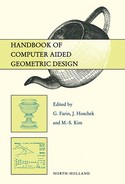
Thus far in this book we have mostly encountered spline curves and surfaces whose parameter domains are subsets of the real line or the Euclidean plane. In particular, in several chapters of this book we became accustomed to the idea that a spline surface is the graph of a bivariate real-valued function or, alternatively, a parametric surface, which is the image of a planar domain under a vector function, or a collection of such functions. The parametric or free-form surfaces that are typically considered in the CAGD literature are composite surfaces consisting of a collection of individual surface patches of the form fi(Si), where
is a three-component vector function whose domain Siis a “simple” planar region, such as the standard triangle or the unit square.
The functions fiare usually chosen to be polynomials of a fixed “low” degree, e.g., Bézier triangles or tensor products of univariate Bernstein polynomials, or rational functions. Moreover, the patches fi(Si) “fit together” so that they form a globally continuous, or even smooth, surface (see Figure 9.1). We refer the reader to Chapters 5, 7, and 8, for a discussion on constructing smooth free-form surfaces with polynomial and rational surface patches.
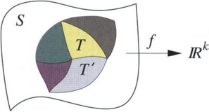
The popularity of polynomial and rational composite surfaces in the CAGD community can be explained by the fact that they can be used to represent, in a robust way, a great variety of shapes and surfaces of arbitrary topological genus. However, in spite of the high flexibility and other attractive properties of such surfaces (see Chapters 4, 5, and 8), in many situations of practical interest it is desirable to extend the above concept of a spline surface a step farther. Namely, it makes sense, at least in principle, to consider the more general case in which the domains Siin (9.1) are non-planar and hence are themselves surfaces. In particular, consider the problem of constructing scalar or vector-valued functions
whose domain Sis a general surface in R3. There are a host of situations in applied sciences where such functions are likely to be useful. Let us briefly mention a few applications. The reader will undoubtedly be able to come up with many other examples on his/her own.
• Scalar Fields. The function f can describe a scalar field associated with the surface S. For example, Scould be the surface of a combustion engine part and f could be the temperature as a function of location on the surface. Or, Scould be the surface of the earth and f one of the following quantities measured at various locations on S: altitude above the sea level, temperature, intensity of the magnetic field, etc. Another example: given values of f measured on S, such as discrete pressures on an aircraft wing, an objective might be to determine the pressure at arbitrary locations on the wing. Yet another application, of interest in CAGD, is when f stands for a scalar field that reflects an aspect of the visual quality of S, such as the Gaussian curvature.
• Vector Fields. A rich source of examples of vector fields defined on surfaces is fluid dynamics. Here the objective is to model/reconstruct velocity fields and other flow quantities that are governed by the Navier-Stokes equations. In particular, in meteorology and global atmospheric modeling, the fluid flow on the surface of the earth is described in terms of the horizontal velocity vector field (with longitudinal and latitudinal components), together with atmospheric pressure [15],[34],[79]. Another example comes from the so-called moving boundary problems in partial differential equations, in which the surface Svaries with time and represents a moving interface between solid and liquid phases of a given material substance, ice and water, say. Typically, the vector field associated with Shas several components, for example the normal vectors to the surface S, its mean curvature, and the velocity of the moving boundary [45].
• Surface Design/Reconstruction. Some surfaces are often closely related to a given “reference” surface Sor are even directly determined by this surface. For example, any scalar field f on Scan be thought of or visualized as a surface in its own right, e.g., the surface
where nsis the unit surface normal at the point s. This is the reason why surfaces of this type are also sometimes referred to as “surfaces on surfaces” [11]. For example, S′ could represent the true surface of the earth, with Sbeing the reference sphere/ellipsoid and f the height above sea level. Or, S′ could be an offset surface to S, i.e., a surface whose distance to Sis a fixed value (in which case the function f in (9.3) is identically equal to this value). In each of these cases it may be advantageous to use Sas a natural parametric domain for S′.
“Surfaces on surfaces” can also be viewed as surfaces in a higher-dimensional space. This is because the set
can be thought of as a two-dimensional manifold imbedded in Rk+3. In particular, if f is a scalar function, then S″ is a two-dimensional surface in four-dimensional Euclidean space.
The first step in most surface reconstruction, modeling, and/or data-fitting problems, aimed at recovering an unknown function f from a set of data or at solving a partial differential equation, is to restrict the class of functions that are used. These restricted classes usually consist of “simple” functions that are suitable for numerical manipulation and at the same time can approximate well other (more general) functions. Thus, we typically work with spline-like or finite-element type functions, which have “piecewise character”, i.e., they belong to a linear space with locally finite dimension. In the context of this chapter, f will be “composed” of functions fi: Si→ Rk(k = 1,2, …), where the Si’s are in general non-planar surfaces tessellating the domain Si.e., S = ∪Si.
At this point, the reader may wonder, and rightly so, whether considering general surfaces Si,. instead of planar ones, is indeed a genuine and worthy generalization of the setting (9.1). This is a legitimate point since, strictly speaking, the general problem (9.2) can in fact be reduced to the simpler case of planar parametric domains. For example, if f is scalar (k = 1) and if we interpret f(S) as the surface S′ in (9.3), then one can use standard parametric polynomial spline techniques to represent/reconstruct f. Alternatively, it is possible to interpret f in the framework (9.4), in which case one could employ (4D) parametric polynomial splines to reconstruct S″ and thereby also f, being the fourth component of S″ (as was done e.g., in [4]). Lastly, in many situations of practical interest, such as in the case of a sphere, the surface Scan be mapped onto a planar region, which again allows us to think of functions defined on Sas functions whose domain is planar. However, we shall see that in many instances it is beneficial to approach a given reconstruction problem in the mind-set of (9.2) and not (9.1). Before we address this point in more detail, it will be instructive to look at some concrete examples.
Example 1.
Although in this chapter we are primarily interested in splines on surfaces, the following example, concerning the modeling of planar curves, will help motivate several important points. In particular, below we describe some interesting facts that arise in the context of designing cam profiles in mechanical engineering.
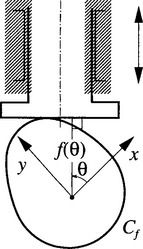
Cams are used in many kinds of mechanical devices. Their basic purpose is to convert rotary motion into linear motion that has a particular displacement as a function of time. Let us restrict ourselves here to cam mechanisms with the so-called flat face follower. The usual way to design a cam profile in this case is to construct the so-called support function f, which describes the displacement of the follower (i.e., the vertical distance of the follower from the center of the cam) as a function of the rotation angle θ, see Figure 9.2. Thus, the support function is a scalar function whose domain Sis the unit circle, parametrized by the polar angle ![]() . The associated profile curve of the cam can be thought of as a parametric curve, i.e., a vector function Cf: S→ R2, whose image is given by
. The associated profile curve of the cam can be thought of as a parametric curve, i.e., a vector function Cf: S→ R2, whose image is given by
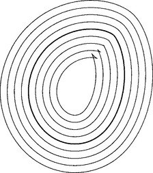
where the Cartesian coordinates satisfy [56]
The objective of cam design is to obtain appropriate support functions f that meet a prescribed set of requirements. Typically, f must take on specific values at given discrete angles and prescribed dwells (i.e., intervals with constant displacement), and should result in a cam that is consistent with the desired behavior of vertical velocity, acceleration, and the so-called jerk.
In principle, to represent f, we could use a piecewise polynomial function that is periodic with period 2π, is sufficiently smooth, and has enough flexibility (i.e., enough knots) to satisfy the various mentioned conditions. However, this would lead to a very complicated representation for the actual cam shape. This is apparent from the above formula for Cf, which is a mixture of polynomial splines and trigonometric functions. In particular, these cam profiles typically do not possess piecewise rational parametrizations as are employed by CAD systems and accepted by CNC milling machines. Conversely, if one desires a (piecewise) polynomial or rational representation for Cf, then the form of the displacement function f is generally far from simple, hence not appropriate for design and optimization purposes.
The mentioned shortcoming of polynomial splines has triggered a search for splines that are better suited to describe functions on the circle. Indeed, in [56] it has been shown that trigonometric splines(i.e., functions consisting of pieces of trigonometric functions, see [69]) are an ideal tool for cam design. In fact, the formula for Cfalone suggests that trigonometric functions play a natural role in representing functions on the circle.
In the context of cam design, trigonometric splines are an attractive alternative to polynomial splines. Namely, representing the support function f as a trigonometric spline leads to a piecewise rational profile curve Cf. Moreover, it turns out that these curves have the remarkable property that their offsets are also piecewise rational [55]. This means that the corresponding cam profiles, as well as the cutter paths for CNC machining, both possess a standard NURBS representation.
The lesson to be learned from this example is that even though polynomial splines can be used to represent functions on the circle, it is more “natural” and advantageous to employ a function space that “matches” the circle, i.e., one that is derived from trigonometric polynomials.
The next example shows that the type of space we use may not be just a question of convenience. In some cases it may also be a matter of necessity.
Example 2
Let us now consider the more difficult problem of constructing smooth functions on the sphere Sin R3. The most obvious approach is to map the sphere onto the plane, using spherical coordinates, then employing classical bivariate tensor-product splines. To state the problem more precisely, suppose that Sis mapped onto the longitude-latitude rectangle
and that f: ω → R is a given function. We can view f as a function on S, provided that it is periodic, that is
and constant at the poles i.e.,
where fsand fNare the values of f at the south and north poles, respectively.
To represent/approximate spherical functions, it is natural to consider the space of tensor-product polynomial splines, i.e., the space of functions of the form
where θiand Φiare univariate B-splines associated with a knot partition of the θ- and φ-xes, respectively. While functions of this form can be made arbitrarily smooth (on Ω) by choosing the degree of the spline sufficiently high, this will not automatically guarantee that f is smooth as a function on S, even if it satisfies both (9.5) and (9.6). In fact, it was shown in [17],[35] (see also [74]) that to obtain a smooth (C1 or higher) function, the following set of equations must hold for the partial derivatives fθand fφ:
and
where AS, BS, AN, and BNare constants. These equations express the condition that f is C1-continuous along the prime meridian θ= 0 and also at the poles, which is equivalent to continuity of the tangent plane of f on S.
It can be seen that, unless the function f is flat at the poles, i.e., unless AS = BS = AN = BN = 0, no tensor-product spline of the form (9.7) can be smooth at the poles. This follows from the fact that the right-hand sides of the last two of the above equalities involve trigonometric polynomials. Thus, no matter how high the degree or fine the knot partition of the longitude-latitude axes, piecewise polynomials are inherently incompatible with the sphere, at least in the above-described setting.
Consequently, to obtain globally smooth spherical functions, we must abandon the idea of using the classical B-splines. Like in our previous example, it is a good idea to utilize trigonometric splines. More precisely, it was shown in [71] that by replacing the B-splines θiin (9.7) with their trigonometric counterparts, it is indeed possible to construct smooth spherical functions of the form (9.7).
The above two examples have demonstrated that the straightforward approach to representing functions on Sis not necessarily optimal. Even if Sis simple enough that it can be mapped onto an interval or a planar region, it may still be useful to “custom-design” a spline space that is compatible with the given surface. As we have seen, in general this will lead to function spaces that are non-polynomial in nature.
A sceptical reader might still argue that there is always the possibility to use standard parametric surface patches, which are piecewise polynomial, to reconstruct f. For instance, in Example 2 we could use parametric surface patches to model the surface S′ in (9.3) and then obtain the corresponding scalar function as f(s) = (S′(s) − s) ˙ ns, ∈ S. While this is true in principle, there are several difficulties associated with this approach. First, using parametric surfaces requires working with vector-valued functions, as opposed to the simpler scalar functions. Second, constructing smooth composite parametric surfaces is a highly non-trivial task since the smoothness conditions between adjoining surface patches are more difficult to impose than in the scalar case. Third, the construction of the parametric surface must guarantee that S′ is star-like, i.e., such that every half-line emanating from the origin intersects S′ only once, for otherwise f would not be well defined. Lastly, once S′ has been constructed, to recover f(s) for a given point s on the sphere, it is necessary to compute the value S′(s). This is a difficult task since it requires solving a set of algebraic equations.
The basic question that arises in the context of (9.2) is how to construct spline spaces of functions on Sthat resemble the usual spaces of piecewise polynomials in the plane (if this is indeed possible). Another important question is whether the well-established data fitting and modeling techniques for functions in the plane can be extended to the general setting of arbitrary surfaces. The hope is that many of the usual methods would carry over to this general situation without too much extra effort.
To address these questions, we will primarily focus our attention in section 9.2 on the issue of constructing spline spaces on S. Alternative approaches to this problem will be listed in section 9.3.
9.2 SCALAR SPLINES ON SMOOTH SURFACES
Having looked at examples of splines on specific manifolds, let us now consider the case of general surfaces. We will first define the context of our setting. In this section the surface Swill be C∞-smooth in the usual sense of differential geometry. This is because our main interest will be in smooth splines on S, which would be an awkward requirement if Sitself were not sufficiently smooth. Of course, for all practical purposes the infinite differentiability condition can be relaxed to match the order of smoothness of f. Also, we will restrict ourselves here to the case of scalar-valued functions f(i.e., k = 1 in (9.2)).
Splines are usually obtained by dividing up the domain of their definition, Sin our case, into disjoint subsets. The most familiar means of partitioning a given domain is to triangulate it. If the domain is planar, the resulting spline space is the well-known space of piecewise polynomials on triangulations. While there exist a great variety of bivariate splines, corresponding to many types of grids and polygonal partitions, piecewise polynomials on planar triangulations are the most universal since all other types can be viewed and represented as splines on triangulations. Therefore, to address the problem on general surfaces S, we will also assume that the sought-for spline space will correspond to a triangulation of S.
As usual, a triangulation of Sis a collection Δ of geodesic triangles on S, whose interiors are disjoint and such that the union of all triangles in Δ is S, i.e., S = ∪T∈ΔT. Here, a geodesic triangle T is a closed subset of S, homeomorphic to a planar triangle, whose boundary consists of three geodesic segments on Sconnecting a triple of points in T, called the vertices of T. These three geodesics are the edges of T. The vertices of T will be denoted by V(T) and the edges by E(T). The edges will be indexed by V(T) such that ev∈ E(T) will denote the edge of T opposite to v∈ V(T).
Perhaps the most popular way of representing splines on triangulations is by means of the Bernstein-Bézier formalism. Bernstein-Bézier techniques are extremely useful tools for constructing piecewise polynomial surfaces over triangulated planar domains. As is demonstrated in many chapters of the book (see chapter 4), they play an important role in CAGD, data fitting, computer vision, and elsewhere (see [22],[39]). To define analogs of Bernstein-Bézier techniques associated with S, we need to find finite-dimensional spaces of functions that play the role of ordinary polynomials in the plane. This in turn leads us to the question of defining an appropriate counterpart of the space of linear functions, since then higher-degree “polynomials” will be obtained as products of the “linear” functions. To be able to express such generalized polynomials in a Bernstein-Bézier-like form, in every triangle T ∈ Δ, we also need to find analogs of the well-known barycentric coordinates. Such generalized coordinates will be denoted as
This reduces the problem of an appropriate definition of “piecewise polynomials” on Δ to finding a reasonable way to define the functions bTv. To answer this query, let us list some of the main properties associated with the classical Bernstein-Bézier formalism:
(1) Non-negativity and partition of unity of Bernstein polynomials associated with any given triangle;
(3) Reproduction of algebraic polynomials;
(4) Affine invariance i.e., Bézier coefficients will not change after transforming the Euclidean plane by an affine transformation;
(5) The possibility of obtaining arbitrarily smooth piecewise polynomials on any triangulation;
(6) Smoothness between adjacent Bézier triangles can be expressed in terms of local Bézier coefficients, corresponding to these triangles.
While this may seem somewhat surprising, in the context of splines on general surfaces the most fundamental of the above items turn out to be properties (5) and (6). That is, spline spaces on general surfaces should be such that they can be used to build functions that are arbitrarily globally smooth (provided the degree is sufficiently high) and yet these spaces should be flexible enough so that it is possible to construct local methods of reconstruction. Another important property of the classical piecewise polynomials, that should be maintained in the general case, is that they are generated in a simple way from linear functions on each triangle. In our setting, the analog of the space of linear functions will be the three-dimensional space LT, which is the linear span of the barycentric coordinates, i.e., LT:= span{bTv, v∈ V(T)].
It is not difficult to see that the spaces LT cannot be quite arbitrary. In particular, the barycentric coordinates should interpolate at the vertices, and in fact
This implies that LT restricted to any of the three edges of T is two dimensional, rather than three dimensional. In addition, a requirement for global continuity (C0) of a spline function in the “linear” spline space
is that the spaces LT|eand LT′|e, corresponding to any pair of neighboring triangles T and T′, sharing a common edge e = T ∩ T′, should be identical, i.e.,
Otherwise it would be impossible to join two neighboring triangular patches in this (or any induced higher-degree) spline space continuously, let alone smoothly.
Assuming that all spaces LT, T ∈ Δ, satisfy (9.8) and (9.9), we can define the space of continuous splines of degree n on Sas
where pTnis the space of “polynomials” of degree n on T ∈ Δ, defined as
and where Bn,Tiare the “Bernstein polynomials” or B-polynomials
for every multi-index i = (iv)v∈V(T)with ![]() . Note that the B-polynomials reduce to the ordinary (algebraic) polynomials if bTvare the usual barycentric coordinates associated with a planar triangle T. Also note that
. Note that the B-polynomials reduce to the ordinary (algebraic) polynomials if bTvare the usual barycentric coordinates associated with a planar triangle T. Also note that
and that the B-polynomials are linearly independent (hence form a basis for PTn), as a consequence of (9.8).
Do conditions (9.8) and (9.9) guarantee that the spaces S0n(Δ), n>1, will automatically contain nontrivial smooth functions, C1say? It should not come as a surprise that the answer is negative. This can be seen in the planar case S = R2 if we choose a set of non-standard functions bTv. Intuitively, the reason for this is that conditions (9.8) and (9.9) do not enforce compatibility of derivatives of these functions across the edges of the triangulation.
Example 3
In Example 2, the sphere Swas parametrized using the spherical coordinates. An alternative is to parametrize Sby the standard octahedron with vertices v1 = (0,0,1), v2 = (1,0,0), v3 = (0,1,0), v4 = (−1,0,0), v5 = (0, −1, 0), v6 = (0, 0, −1) (or by any polyhedron inscribed in S). The vertices of the octahedron give rise to a triangulation Δ of the sphere, consisting of eight spherical triangles. Consider two adjacent triangles in Δ, say T and T′, determined by their vertices V(T) = {v1, v3, v2} and V(T′) = {v1, v3, v4}, respectively. Let us now define the functions bTv, bT′vfor the two triangles as the usual barycentric coordinates associated with the planar triangles with vertices V(T) and V(T′). One can check that this leads to
where s = (x, y, z) ∈ T′. The reader is invited to verify that (9.8) and (9.9) are satisfied in this case. However, given a function f ∈ PT2, it may be impossible to find an f′ ∈ PT′2such that the two functions join smoothly (C1) across the common edge v1v3(for example, take f = (bTv1)2).
The following proposition gives a necessary condition for a smooth join between neighboring triangles [54].
Proposition 1
Let T, T′ ∈ Δ be two adjacent triangles on Ssuch that T ∪ T′ is homeomorphic to a disk in R2. Let bTv∈ C∞(T), v∈ V(T), and bT′v∈ C∞(T′), v∈ V{T′). Suppose that for every n and every f ∈ PTnthere exists an f′ ∈ PT′nsuch that f and f′ join with Cn−1 continuity along the common edge T ∩ T′. Then each bTv∈ T, can be extended as a C∞ function on T ∪ T′ which, when restricted to T′, belongs to LT′. Equivalently, there exists a three-dimensional space L of C∞ functions on T ∪ T′ such that L|T = LT an d L|T′ = LT′.
A consequence of this result is that the choice of the functions bTvis greatly restricted. In particular, the proposition says that all barycentric coordinates bTvcorresponding to any given triangle T, can be smoothly extended across edges of T to neighboring triangles and hence all spaces LT must locally belong to a single three-dimensional space of “linear functions” L. The following example shows that such a space L might not contain globally continuous functions, i.e., for some surfaces one may be able to define L only locally.
Example 4
Let Sbe the circular cylinder parametrized by
and let
Hence, the point on Swhose parameters are (φ, z) is assigned the value a + bφ + cz, where a, b, c are real coefficients. Note that L is not defined globally since there is no globally continuous function in it. However, on every “strip”
where β– α≤ 2π, the space L is well defined and generated by C∞ functions.
If Δ is a geodesic triangulation of Sconsisting of “small” triangles (i.e., triangles for which the values of φare in an interval of length not exceeding pI), then it is not difficult to see that for every such triangle T, dim(LT|e) = 2, e ∈ E(T), where LT:= L|T. This follows from the observation that every f ∈ L vanishes along geodesics. Namely, if f(φ, z) = a + bφ + cz, where b ∞ 0, then f(φ, z) = 0 along the curve
which is a helix, hence a geodesic. Otherwise, if b = 0, z is a constant, which also corresponds to a geodesic on S.
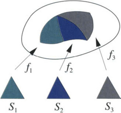
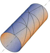
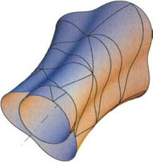
The above discussion shows that for every sufficiently small geodesic triangle T ∈ Δ, one can define cylindrical barycentric coordinates. It turns out that many properties of these coordinates are similar to the properties of their planar counterparts. In particular, the cylindrical barycentric coordinates make it possible to define a spline space, which can be used to construct smooth splines on S. Figure 9.5shows an example of a cylindrical triangulation Δ and Figure 9.6shows a C1 smooth spline in the space S05(Δ), corresponding to this triangulation.
Example 4 raises the question whether a space L, or a collection of spaces LT satisfying the conditions implied by Proposition 1, always exists on any Sand, if so, how can one find such spaces. A simple approach to constructing L is to take advantage of our knowledge of S, i.e., the implicit assumption here that we can evaluate Sat any point. In particular, we can define L as the span of the three functions x(s), y(s), z(s), the Cartesian coordinates of s i.e., s = (x(s), y(s), z(s)), s∈ S. This works well in the important special case of a sphere in R3.
Example 5.
The problem of constructing spherical analogs of Bézier triangles has an interesting history. It has received ample attention in the spline literature for the obvious reason that splines on a sphere have many potential applications in geosciences, including meteorology, geophysics, and geodesy. Researchers had been searching for many years for appropriate spherical analogs of Bézier methods, but were hampered by the difficulty of defining spherical barycentric coordinates. For example, several candidates for such coordinates have been introduced in [13],[14],[41], but they lacked many key properties of the planar coordinates. As it turned out, the mentioned attempts were destined to be unsuccessful for the simple reason that they all insisted on the partition of unity property, which is well known for the classical barycentric coordinates. Namely, it was shown in [14] that spherical barycentric coordinates that sum to one and satisfy a list of other reasonable assumptions, do not exist. This negative result provided an explanation why the various earlier generalizations were unsuccessful in building smooth splines on spherical triangulations.
A breakthrough in this development came when the authors of [1] realized, by studying identities of spherical trigonometry, that there is in fact a natural way of defining barycentric coordinates for spherical triangles. Let T be a spherical triangle with vertices v1, v2, v3∈ S. Thus the edges of T are the three shortest geodesies connecting the vertices. One can define the spherical barycentric coordinates of a point s∈ T as
where Δiis the geodesic distance (measured along the great circle passing through s and Vi) of uiand s, and γiis the geodesic distance of s and Vi(see Figure 9.7).
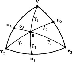
Despite the inevitable fact that the above coordinates do not add up to one, it has been shown in [1] that they resemble the standard barycentric coordinates in many respects. First, the barycentric coordinates are infinitely smooth functions on T and they satisfy (9.8). The space LT, the span of the three coordinates, reduces to dimension two along the edges of T and in fact along every great circle intersecting T. More precisely, the restriction of LT to any such great circle can be shown to be the linear span of {sin α, cos α}, where αis the arclength distance measured along this circle. Another important consequence of the above definition is that the spaces LT and LT′, associated with neighboring triangles T and T′, satisfy (9.9). Furthermore, the properties of C7 are consistent with those specified in Proposition 1. In particular, this space can be extended to a three-dimensional space L of infinitely differentiate functions over all of S. Conversely, for any triangle T the space LT is just the restriction of L to T.
The space L has many interesting properties that indicate that spherical barycentric coordinates, as defined here, are unique. More precisely, L is the only three-dimensional space of functions on the sphere Sthat is rotationally invariant and such that its dimension is reduced along great circles. Moreover, L, can be easily described using the idea suggested earlier. Namely, L is precisely the span of the Cartesian coordinates x(s), y(s), z(s), viewed as functions on S. This is equivalent to saying that L is the space of spherical harmonicsof degree one [49].
The intimate connection between spherical harmonics and spherical barycentric coordinates is not unexpected. In retrospect, it seems quite obvious that these functions should have been considered early on as the most natural candidates for “linear functions” on the sphere. As a matter of fact, such functions, along with the corresponding barycentric coordinates defined above, had been considered some 150 years before the paper [1] appeared. The authors of that paper found out only later that their idea of defining barycentric coordinates was not new after all, since the same definition had already been given by Möbius [47].
Spherical barycentric coordinates give rise to Bernstein-Bézier-type methods, with immediate applications to a variety of problems on the sphere. Indeed, because of the close analogy with standard Bernstein-Bézier techniques, virtually all of the classical methods for piecewise polynomials on planar triangulations can be carried over to the spherical setting, and indeed to any setting where barycentric coordinates are available. A detailed treatment of some of these methods has been given in [2],[3]. The spherical Bernstein-Bézier methods are also of interest in the design of surfaces, especially star-like surfaces, even though some of the geometric properties of planar Bézier methods are missing on the sphere, such as the convex hull property.
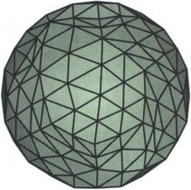
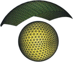
Typical scattered data interpolation/approximation methods on the sphere start with a triangulation of the sphere, for example the so-called Delaunay triangulation. We refer the reader to [69], for a survey on triangulations, and also to [11],[39], for a discussion of triangulation methods on general surfaces. Methods for triangulating scattered data points on the sphere are discussed in [41],[58],[66]. Figures 9.9and 9.10show wire plots of smooth C1 quadratic and cubic spherical splines, respectively, corresponding to (a part of) the triangulation in Figure 9.8. Details about various data-fitting methods that lead to such spherical splines are discussed in [3].
Besides the sphere, the suggestion to use Cartesian coordinates to define the space L makes sense, as long as the triangulation Δ of S consists of triangles whose edges reduce the dimension of L. This is equivalent to the condition that the edges of Δ are planar and in the same plane with the origin (0, 0, 0). This is acceptable for certain surfaces (for example, for star-like surfaces [3]), but is more restrictive in cases in which the assumption of coplanarity would result in severely distorted triangles (relative to the geodesic ones).
To cope with this difficulty, a possibility is to make a coordinate transformation to minimize the distortion of the triangles, e.g., one could shift the origin of the Cartesian system. More generally, one could in principle take “any” three-dimensional space K of smooth functions in R3 and define L as the restriction of H to S. In the spherical case, this would lead to L = H|s, where H:= span{x, y, z}. In the planar case S = R2, we can think of L as H|s, where H:= span{l, x, y}. In this way one can also interpret the construction of L for the cylinder. In particular, we can take for any fixed α∈ R,
in which case L is the restriction of H to the strip
On the other hand, it is not clear how to choose H for a general surface Sso as to obtain “least distorted” triangulations.
Above, we have seen two examples of non-planar surfaces for which it is possible to construct meaningful analogs of spline spaces. The characteristic property shared by both types of splines, as well as by the classical bivariate splines on planar triangulations, is that they can be generated by a three-dimensional space L of “linear functions” on S.
• Functions in L vanish along geodesics on Si.e., for every nontrivial f ∈ L, the set C:= {s∈ S, f(s) = 0} is a geodesic. Conversely, for every geodesic Con S, there exists a nonzero function f ∈ L vanishing on C.
• L is invariant under isometric transformations of S. Thus, if I: S→ Sis an isometry (e.g., a rotation, if Sis the sphere), then f o I ∈ L for all f ∈ L.
It is clear that these two properties imply that L is quite special and that for a given surface Sone cannot expect to have more than one such space. In fact, in the three mentioned cases, L is uniquely determined by the above two properties. It is an intriguing open question whether there always exists a space satisfying at least the first property. This in turn is closely related to the central issue of this section of whether one can find analogs of spline spaces on general surfaces. Using the well-known Beltrami’s Theorem about the existence of local geodesic mappings [18], it can be shown that L can be found for surfaces of constant (Gaussian) curvature [54]. However, it is not known if one can go beyond such surfaces.
It should be said that, for all practical purposes, we need not require that L strictly satisfy the mentioned conditions. The lack of a theoretical proof of the existence of L should not prevent us from being able to establish useful spline spaces on S. For example, for a given fixed geodesic triangulation Δ, one could use a space L which has a reduced dimension along all of its edges, but which does not necessarily have the property that all functions in L vanish along geodesics. Such space L will still allow the construction of barycentric coordinates for all triangles of Δ, hence also the construction of a spline space corresponding to Δ.
Another possibility is to relax the assumption that the triangles in Δ are strictly geodesic. In fact, parametric surfaces Scomposed of triangular Bézier patches are already equipped with a natural triangulation Δ in which every triangle corresponds to a Bézier patch. Such a triangulation is in general not geodesic. In this situation there is a particularly simple way to choose the barycentric functions bTv. Recall that Example 3gives reasons why it is in general not a good idea to use the standard barycentric coordinates corresponding to the triangular facets of the piecewise linear interpolant to the vertices of Δ. This is because this will in general not permit us to design smooth splines over S. However, it turns out that this approach will work if Sis a composite surface consisting of triangular polynomial patches. Namely, the fact that neighboring triangular patches are joined smoothly guarantees that the ordinary planar barycentric coordinates corresponding to these triangles are compatible, in the sense of Proposition 1. Thus in any given triangle these coordinates can be extended to the neighboring triangles as smooth functions (where the degree of smoothness will depend on the smoothness of S).
We have seen that the success or failure of constructing spline spaces on general surfaces hinges upon the existence of barycentric coordinates. It is also clear from our examples, that even for simple surfaces such constructions may be far from trivial. Still, the discussed framework of splines on surfaces offers many benefits, compared to other existing reconstruction methods. The main argument supporting this claim is that the Bernstein-Bézier formalism for splines on surfaces is the same for all surfaces. That is, it is essentially irrelevant whether we work on the sphere, in the plane, or on any other surface. As a consequence, we can use the same algorithms for splines on all surfaces, as long as we use a correct procedure to compute the barycentric coordinates (which do depend on the type of the surface).
Example 6.
To illustrate the above point, suppose that T, T′ ∈ Δ are two adjacent triangles on S, with vertices V(T) = {v1, v3, v2} and V(T′) = (v1, v2, v3). Let f and f′ be two “polynomials” of degree n of the form
where cTi, cT′i∈ R are given Bézier coefficients. Then f and f′ join continuously along the edge V1v3if
and they join with C1 continuity if and only if
where we used the abbreviations ij:= ivj, j = 1, 2, 3. Moreover, the values bTvi(v4) are obtained by first extending bTvj. as smooth functions to T ∪ T′, and then evaluating them at v4. This extension is possible as long as the barycentric coordinates are compatible in the sense of Proposition 1.
The above conditions for a smooth join between two generalized Bézier triangles can be immediately seen to be formally identical to the corresponding conditions in the planar setting. This explains why we have not addressed in this section the actual reconstruction problem (e.g., interpolation or approximation) using splines on surfaces. The reason is that the same methods known in the plane can be transformed almost automatically to any surface. Various extensions of such planar methods to the sphere are discussed in [3] and it is indeed clear from that paper that, except for a few details, the planar methods carry over to the spherical setting, and indeed to the setting of any smooth surface S.
9.3 ALTERNATIVE METHODS FOR FUNCTIONS ON SURFACES
In this chapter our focus was mainly on discussing splines on surfaces, i.e., analogs of piecewise polynomials on planar triangulations. However, this should not leave the reader with the impression that there are not other methods that have been used successfully in data-fitting and reconstruction problems on surfaces. Therefore, in this section we will give a brief description of other available methods and provide references for further study. This is also a good place to mention other surveys that have been written on the topic of splines on surfaces, such as Chapter 9.7in [39] and [8].
9.3.1 Discrete surfaces
Having discussed the idealized problem in which Swas a smooth surface, it should be mentioned that in some applications surfaces come as discrete collections of points. For example, Sand f could be sampled at a set of discrete points si∈ R3, where the sicould represent the triple (latitude, longitude, altitude), determining a physical location on the surface of the earth and ficould be the air pressure at si. Before we can find an approximation to f using the setting described in the previous section, we first need a preprocessing step for reconstructing the surface S. We refer the reader to chapter 26in this book and also to [7],[11],[39],[46],[75], for an overview of and references on several methods for surface reconstruction from scattered data points in R3.
9.3.2 Radial basis functions
An increasingly popular class of methods for interpolation and approximation of scattered data are those based on radial basis functions(RBF), i.e., functions that are radially symmetric. The reason why such methods are often preferred to other techniques is that these methods are meshless. This means that to interpolate a set of functional data associated with scattered points on a surface it is not necessary to create a triangulation, or any other type of mesh that connects the given data sites, prior to the actual reconstruction phase.
Perhaps the first types of radial basis functions used in the context of interpolation of functions on surfaces were the Hardy multiquadrics, introduced for application in geophysics in [36–38] (see also [8],[21],[26],[62]). The advantage of using radial basis functions over other methods in the setting of functions on surfaces is that a given function is approximated and/or interpolated by a linear combination of translates of a single RBF, which gives a very simple representation of the resulting reconstruction.
Many papers have been written on the use of RBFs in the spherical setting, see [23],[24], [62],[72], and also the survey [25]. Recently, RBFs on the sphere have been employed not only in the context of interpolation but also the context of solving differential equations on the sphere [48]. There are also several papers on Lagrange and Hermite interpolation on general Riemannian manifolds [19],[20],[50], which are of interest for functions on surfaces of arbitrary topology.
Methods based on RBFs generally suffer from poor conditioning of the linear systems that arise in interpolating large sets of data. However, lately there has been considerable progress on compactly supported RBFs (see [25]), which have the potential to reduce this shortcoming of RBFs.
9.3.3 Variational methods
A well–established approach to constructing bivariate functions interpolating scattered data in the plane is to use the so–called variational methods, which are based on minimizing an “energy functional” subject to given interpolation conditions. Strictly speaking, variational methods belong to the previous subsection since the kernels associated with such extremal problems are also radially symmetric. The methods have been frequently used in geosciences, see [29–31],[33],[76–78]. Another popular method, often applied in meteorology, is the classical spectral method. This method uses spherical harmonics of high degrees to approximate functions defined on the sphere [44].
9.3.4 Distance-weighting methods
This class of methods, sometimes also called Shephard-type methods, uses a weighted combination of function values that are being interpolated on the surface S, to reconstruct an unknown function from discrete data. The weights are chosen so as to decrease the influence of a particular data point on the surface as we move away from this point. In this way points that are far from a given region on the surface will have little or no effect on the reconstructed function in that region. For details on how to choose the weight functions, we refer the reader to [11],[12] and Chapter 9.7of [39].
9.3.5 Transfinite methods
Many techniques for defining functions on triangulated (or otherwise partitioned) surfaces are based on the idea of transfinite interpolation. This method starts with the construction of a network of smooth functions defined on the edges of the partition and then uses transfinite triangular interpolants to interpolate the network of curves by a smooth function on the domain surface S. The papers [11],[10],[40],[41],[58],[67] describe a construction of such transfinite triangular interpolants for the sphere, whereas [61] can be applied to arbitrary surfaces that are at least C2 differentiate.
9.3.6 Implicit methods
In [5–7], implicit Bernstein-Bézier patches (also called A-patches) are used to simultaneously reconstruct the surface S(given as a set of unorganized points) and the unknown function f, whose values at these points are given. An advantage of this method is that it does not require any assumption on the convexity and/or differentiability of Sand that it can handle oriented manifolds of unrestricted topological types. On the other hand, the drawback of using implicit surface patches is that they require essentially trivariate Bernstein-Bézier techniques, which are harder to deal with than bivariate ones.
9.3.7 Other types of splines
Besides splines on triangulations of a surface S, various other types of splines can be constructed. For example, the papers [52],[60] give a construction of spherical simplex splines. A recent introduction on simplex splines is [53]. The paper [42] uses spherical splines on triangulations to define hybrid cubic Bézier patches, which are analogs of the classical rational Bézier patches. The author is not aware of similar methods for other types of surfaces (except planar).
9.3.8 methods
This overview would be incomplete if we did not mention the possibility of using subdivision or wavelet-type methods in connection with the reconstruction of functions on surfaces. Subdivision methods are a powerful means of constructing surfaces and hence one would expect that they might also lend themselves to problems in the area of “surfaces on surfaces”. There is no question that wavelet and subdivision techniques are becoming increasingly popular in many application areas, ranging from signal and image processing to CAGD and computer animation. That said, there do not seem to exist many methods based on subdivision and/or wavelets designed specifically to deal with the problem of functions on surfaces. Notable exceptions are the various existing constructions of wavelets on the sphere (see [16,32,33,43,51,68]) and the paper [73], where wavelets are constructed on general surfaces.
9.3.9 Visualization of surfaces on surfaces
Although visualization is not addressed in this chapter, it is important to stress that a good visualization of the reconstructed/modeled surfaces and functions is essential in the context of functions on surfaces since, as we have pointed out earlier, these surfaces can be viewed as being imbedded in a higher-dimensional space. Therefore, an appropriate technique to display the results of the reconstruction can significantly enhance our understanding of the behavior of the reconstructed functions and surfaces. While visualizing a surface in the four-dimensional space is very difficult, there are ways to display them by a judicious use of interactive color computer graphics. The topic of visualization of such surfaces is discussed at length in many publications, including [4],[9],[28],[57],[59],[63–65].
1. Alfeld, P., Neamtu, M., Schumaker, L.L. Bernstein-Bézier polynomials on spheres, and sphere-like surfaces. Computer Aided Geometric Design. 1996;13:333–349.
2. Alfeld, P., Neamtu, M., Schumaker, L.L. Dimension and local bases of homogeneous spline spaces. SIAM J. Math. Anal. 1996;27:1482–1501.
3. Alfeld, P., Neamtu, M., Schumaker, L.L. Fitting scattered data on sphere-like surfaces using spherical splines. J. Comp. Appl. Math. 1996;73:5–43.
4. Bajaj, C., Xu, G. Modeling and visualization of scattered function data on curved surfaces. In: Chen J., Thalmann N., Tang Z., Thalmann D., eds. Fundamentals of Computer Graphics. Berlin: World Scientific Publishing Co.; 1994:19–29.
5. Bajaj, C., Bernardini, F., Xu, G., Automatic reconstruction of surfaces and scalar fields from 3D scans. Proceedings of SIGGRAPH 95. Computer Graphics, Annual Conference Series. ACM SIGGRAPH, 1995:109–118.
6. Bajaj, C., Bernardini, F., Xu, G. Adaptive reconstruction of surfaces and scalar fields from densescattered trivariate data. Computer Science Technical Report, TR 95-028, Purdue University. 1995.
7. Bajaj, C., Bernardini, F., Xu, G. Reconstruction of surfaces and surfaces-on-surfaces from unorganized weighted points. Algorithmica. 1997;19:243–261.
8. Barnhill, R.E., Foley, T.A. Methods for constructing surfaces on surfaces. In: Hagen H., Roller D., eds. Geometric Modeling, Methods and Applications. Springer; 1991:1–15.
9. Barnhill, R.E., Makatura, G.T., Stead, S.E. A new look at higher dimensional surfaces through computer graphics. In: Farin G.E., ed. Geometric Modeling: Algorithms and New Trends. Berlin: SIAM; 1987:123–130.
10. Barnhill, R.E., Opitz, K., Pottmann, H. Fat surfaces: a trivariate approach to triangle-based interpolation on surfaces. Computer Aided Geometric Design. 1992;9:365–378.
11. Barnhill, R.E., Ou, H.S. Surfaces defined on surfaces. Computer Aided Geometric Design. 1990;7:323–336.
12. Barnhill, R.E., Piper, B.R., Rescorla, K.L. Interpolation to arbitrary data on a surface. In: Farin G.E., ed. Geometric Modeling: Algorithms and New Trends. Philadelphia: SIAM; 1987:281–290.
13. Baumgardner, J.R., Frederickson, P. Icosahedral discretization of the two-sphere. SIAM J. Numer. Anal. 1985;22:1107–1115.
14. Brown, J.L., Worsey, A.J. Problems with defining barycentric coordinates for the sphere. Mathematical Modelling and Numerical Analysis. 1992;26:37–49.
15. Browning, G.L., Hack, J.J., Swarztrauber, P.N. A comparison of three numerical methods for solving differential equations on the sphere. Mon. Weather Rev. 1989;117:1058–1075.
16. Dahlke, S., Dahmen, W., Weinreich, I., Schmitt, E. Multiresolution analysis and wavelets on S2 and S3. S3 Numer. Fund. Anal. Optimiz. 1995;16:19–41.
17. Dierckx, P. Algorithms for smoothing data on the sphere with tensor product splines. Computing. 1984;32:319–342.
18. do Carmo, M.P. Differential Geometry of Curves and Surfaces. Philadelphia: Prentice-Hall; 1976.
19. Dyn, N., Narcowich, F.J., Ward, J.D. A framework for interpolation and approximation on Riemannian manifolds. In: Approximation Theory and Optimization, (Cambridge, 1996). New Jersey: Cambridge Univ. Press; 1997:133–144.
20. Dyn, N., Narcowich, F.J., Ward, J.D. Variational principles and Sobolev-type estimates for generalized interpolation on a Riemannian manifold. Constr. Approx. 1999;15:175–208.
21. Eck, M. MQ-curves are curves in tension. In: Mathematical Methods in Computer Aided Geometric Design, II (Biri, 1991). Cambridge: Academic Press; 1992:217–228.
22. Farin, G. Curves and Surfaces for Computer Aided Geometric Design, 4th Edition. Boston, MA: Academic Press; 1996.
23. Fasshauer, G.E. Adaptive least squares fitting with radial basis functions on the sphere. In: Dæhlen M., Lyche T., Schumaker L.L., eds. Mathematical Methods for Curves and Surfaces. Boston: Vanderbilt University Press; 1995:141–150.
24. Fasshauer, G.E. Hermite interpolation with radial basis functions on spheres. Adv. Comput. Math. 1999;10:81–96.
25. Fasshauer, G.E., Schumaker, L.L. Scattered data fitting on the sphere. In: Dæhlen M., Lyche T., Schumaker L.L., eds. Mathematical Methods for Curves and Surfaces II. Nashville: Vanderbilt Univ. Press; 1998:117–166.
26. Foley, T.A. Interpolation to scattered data on a spherical domain. In: Mason J.C., Cox M.G., eds. Algorithms for Approximation II. Nashville: Chapman & Hall; 1990:303–310.
27. Foley, T.A., Lane, D.A., Nielson, G.M., Franke, R., Hagen, H. Interpolation of scattered data on closed surfaces. Computer Aided Geometric Design. 1989;7:303–312.
28. Foley, T.A., Lane, D.A., Nielson, G.M., Ramaraj, R. Visualizing functions over a sphere. IEEE Comp. Graphics & Appl. 1990;10:32–40.
29. Freeden, W. On spherical spline interpolation and approximation. Math. Meth. Appl. Sci. 1981;3:551–575.
30. Freeden, W. Spherical spline interpolation-basic theory and computational aspects. J. Comp. Appl. Math. 1985;11:367–375.
31. Freeden, W., Gervens, T., Schreiner, M. Constructive Approximation on the Sphere With Applications to Geomathematics. London: Oxford University Press; 1998.
32. Freeden, W., Schreiner, M. Orthogonal and nonorthogonal multiresolution analysis, scale discrete and exact fully discrete wavelet transform on the sphere. Constr. Approx. 1998;14:493–515.
33. Freeden, W., Schreiner, M., Franke, R. A survey on spherical spline approximation. Surveys Math. Indust. 1997;7:29–85.
34. Giraldo, F.X. Lagrange-Galerkin methods on spherical geodesic grids: the shallow water equations. J. Comput. Phys. 2000;160:336–368.
35. Gmelig Meyling, R.H.J., Pfluger, P. B-spline approximation of a closed surface. IMA J. Numer. Anal. 1987;7:73–96.
36. Hardy, R.L. Multiquadric equations of topography and other irregular surfaces. J. Geophysical Res. 1971;76:1905–1915.
37. Hardy, R.L., Göpfert, W.M. Least squares prediction of gravity anomalies, geoidal undulations, and deflection of the vertical with multiquadric harmonic functions. Geophy. Res. Letters. 1981;2:423–426.
38. Hardy, R.L., Nelson, S.A. A multiquadric-biharmonic representation and approximation of disturbing potential. Geophys. Res. Letters. 1986;13:18–21.
39. Hoschek, J., Lasser, D. Fundamentals of Computer Aided Design. Oxford: AK Peters; 1993.
40. Rpt. 487 Lawson, C.L. Subroutines for C1 surface interpolation to data defined over the surface of a sphere. Boston: JPL, Cal. Tech.; 1982.
41. Lawson, C.L. C1 surface interpolation for scattered data on a sphere. Rocky Mountain J. Math. 1984;14:177–202.
42. Liu, X., Schumaker, L.L. Hybrid cubic Bézier patches on spheres and sphere-like surfaces. J. Comput. Appl. Math. 1996;73:157–172.
43. Lyche, T., Schumaker, L.L. A multiresolution tensor spline method for fitting functions on the sphere. SIAM J. Sci. Comp. 2000;22:724–747.
44. Machenhauer, B., The spectral method. Numerical Methods Used in Atmospheric Models. vol. II of GARP Pub. Ser. No. 17. JOC, World Meteorological Organization, 1979:121–275.
45. Mayer, U. A numerical scheme for moving boundary problems that are gradient flows for the area functional. European J. Appl. Math. 2000;11:61–80.
46. Mencl, R., Müller, H. Interpolation and approximation of surfaces from three- dimensional scattered data points. In: Scientific Visualization, Dagstuhl’97. Geneva, Switzerland: IEEE Publishers; 2000.
47. Möbius, A.F. Ueber eine neue Behandlungsweise der analytischen Sphärik. In: Abhandlungen bei Begründung der Königl. Sächs. Gesellschaft der Wissenschajten. Jablonowski Gesellschaft; 1846:45–86. Möbius, A.F. [Reappeared in Klein, F. Gesammelte Werke, 1886:1–54. [Leipzig].
48. T. Morton and M. Neamtu. Error bounds for solving pseudodifferential equations on spheres by collocation with zonal kernels. To appear in J. Approx. Theory.
49. Müller, C., Spherical Harmonics. Lecture Notes in Mathematics, vol. 17. Springer-Verlag: Leipzig, 1966.
50. Narcowich, F.J. Generalized Hermite interpolation and positive definite kernels on a Riemannian manifold. J. Math. Anal. Appl. 1995;190:165–193.
51. Narcowich, F.J., Ward, J.D. Nonstationary wavelets on the m-sphere for scattered data. Appl. Comput. Harmon. Anal. 1996;3:324–336.
52. Neamtu, M. Homogeneous simplex splines. J. Comp. Appl. Math. 1996;73:173–189.
53. Neamtu, M. What is the natural generalization of univariate splines to higher dimensions? In: Lyche T., Schumaker L.L., eds. Mathematical Methods for Curves and Surfaces: Oslo 2000. Berlin-Heidelberg: Vanderbilt University Press; 2001:355–392.
54. M. Neamtu Barycentric coordinates defined on surfaces. In preparation
55. Neamtu, M., Pottmann, H., Schumaker, L.L. Dual focal splines and rational curves with rational offsets. Math. Eng. Ind. 1998;7:139–154.
56. Neamtu, M., Pottmann, H., Schumaker, L.L. Designing NURBS cam profiles using trigonometric splines. J. Mech. Des. 1998;120:175–180.
57. Nielson, G.M. Modeling and visualizing volumetric and surface-on-surface data. In: Hagen H., Mueller H., Nielson G., eds. Focus on Scientific Visualization. Nashville, TN: Springer-Verlag; 1992:219–274.
58. Nielson, G.M., Ramaraj, R. Interpolation over a sphere based upon a minimum norm network. Computer Aided Geometric Design. 1987;4:41–58.
59. Opitz, K., Pottmann, H. Computing shortest paths on polyhedra: applications in geometric modeling and scientific visualization. Int. J. Comp. Geom. Applic. 1994;4:165–178.
60. Pfeifle, R.N., Seidel, H.-P., Spherical triangular B-splines with application to data fitting. Proc. Eurographics. 1995:89–96.
61. Pottmann, H. Interpolation on surfaces using minimum norm networks. Computer Aided Geometric Design. 1992;9:51–67.
62. Pottmann, H., Eck, M. Modified multiquadric methods for scattered data interpolation over a sphere. Computer Aided Geometric Design. 1990;7:313–321.
63. Pottmann, H., Hagen, H., Divivier, A. Visualizing functions on a surface. Journal of Visualization and Computer Animation. 1991;2:52–58.
64. Pottmann, H., Opitz, K. Curvature analysis and visualization for functions defined on Euclidean spaces or surfaces. Computer Aided Geometric Design. 1994;11:655–674.
65. Ramaraj, R. Interpolation and display of scattered data over a sphere. MS thesis, Arizona State University. 1986.
66. Renka, R.J. Interpolation of data on the surface of a sphere. ACM Trans. Math. Software. 1984;10:417–436.
67. Renka, R.J. Algorithm 623: Interpolation on the surface of a sphere. ACM Trans. Math. Software. 1984;10:437–439.
68. Schröder, P., Sweldens, W., Spherical wavelets: Efficiently representing functions on the sphere. Proceedings of Siggraph. 1995.
69. Reprinted by Krieger, Malabar, Florida, 1993 Schumaker, L.L. Spline Functions: Basic Theory. Berlin: Interscience; 1981.
70. Schumaker, L.L. Triangulation methods in CAGD. IEEE Computer Graphics and Applications. 1993;13:47–52.
71. Schumaker, L.L., Traas, C.R. Fitting scattered data on spherelike surfaces using tensor products of trigonometric and polynomial splines. Numer. Math. 1991;60:133–144.
72. Svensson, S.L. Finite elements on the sphere. J. Approx. Theory. 1984;40:246–260.
73. Sweldens, W. The lifting scheme: a construction of second generation wavelets. SIAM J. Math. Anal. 1998;29:511–546.
74. Traas, C.R. Smooth approximation of data on the sphere with splines. Computing. 1987;38:177–184.
75. Veltkamp, R., Closed object boundaries from scattered points. Lecture Notes in Computer Science, 885. Springer-Verlag: New York, 1994.
76. Wahba, G. Spline interpolation and smoothing on the sphere. SIAM J. Sci. Statist. Comput., 1981;2:5–16. Wahba, G. Spline interpolation and smoothing on the sphere [Errata]. SIAM J. Sci. Statist. Comput. 1982;3:385–386.
77. Wahba, G. Vector splines on the sphere, with application to the estimation of vorticity and divergence from discrete, noisy data. In: Schempp W., Zeller K., eds. Multivariate Approximation Theory II. Berlin: Birkhäuser; 1982:407–429.
78. Wahba, G. Surface fitting with scattered noisy data on Euclidean d- spaceand on the sphere. Rocky Mountain J. Math. 1984;14:281–299.
79. Williamson, D.L., Browning, G.L. Comparison of grids and difference approximations for numerical weather prediction over a sphere. J. Appl. Meteor. 1973;12:264–274.