
Direct Rendering of Freeform Surfaces
Freeform geometry has been employed in computer graphics for more than three decades. Traditionally, the rendering of freeform surfaces has been preceded by a stage in which a piecewise linear polygonal approximation is derived from the original surfaces, leaving polygons to participate in the actual rendering process.
This chapter considers some recent results on the direct rendering of freeform geometry: in other words, the rendering of freeform curves and surfaces without resorting to piecewise linear approximations.
30.1 INTRODUCTION
Surface rendering is traditionally conducted with the aid of a piecewise linear approximation. Usually, curves are sampled and displayed as polylines and surfaces are approximated by polygons. Rendering of the resulting piecewise linear data is expected to be numerically more stable and is supported by contemporary hardware: finding the intersection between a light ray and a polygon is relatively straightforward. In contrast, computing the intersection between a ray and a polynomial surface is difficult, because it amounts to root finding. With the exception of trivial cases, roots must be found numerically. At the same time, the robustness of the rendering algorithm must be guaranteed. A failure of one computation in a million is unacceptable as even one wrong-colored pixel in the picture may be noticeable. The human visual system is surprisingly sensitive and is able to detect such minor defects and hence demands this extreme level of robustness.
Rendering techniques may be classified into several basic computational approaches. The simplest approach is to scan-convert the polygonal data set into a Z-buffer [15]. Each polygon, in the discrete image space, is converted into the set of pixels that approximately covers it. Then, the depth of each pixel is compared against the depth of the corresponding pixel already in the Z-buffer, and only the one at the front is kept. This approach is quitesimple and is nowadays implemented in hardware, even with PC-based systems.
Ray-tracing [16] is another common rendering method. Here, a (primary) ray is traced back from the eye, through a pixel in in the image plane, and towards the scene. If the ray hits nothing, a background color is assigned to that pixel. Otherwise, let us assume the ray hits an object O If O is reflective, a reflected ray is emitted from the intersection point on the surface of O. If O is translucent, then a refracted ray is emitted into O, following Snell’s law [15]. The final color of the pixel corresponding to the primary ray results from the accumulated contributions of the different surface properties of O, including reflectivity, translucency, O’s own color, the illumination, the surface normal of O at that point, and so on.
Another rendering scheme, known as the Radiosity method [15], attempts to evaluate the exchange of light energy among all the surfaces in the scene. In this technique, the scene is subdivided into small differential area elements and a large set of linear equations is set up to express the exchange of light energy between every pair of elements. An approximate solution to this large set of linear equations is typically found using iterative methods, starting from the objects in the scene that represent the light sources.
All the above rendering methods, as well as many of their derivatives, have already been very successful in the context of polygonal geometry. But the topic of this chapter is their adaptation for the direct rendering of freeform geometry. We seek to eliminate the need for a piecewise linear approximation to feed the rendering pipeline, opening the way for the renderer to process the original freeform geometry. By doing so, we expect to gain in three different ways. Firstly, direct rendering of freeform surfaces is likely to be much more precise, because any piecewise linear representation is merely an approximation. Secondly, a single freeform surface, that can be expressed using a few dozen coefficients, has typically to be approximated using thousands of polygons in order to achieve reasonable accuracy. The direct use of freeform geometry potentially eliminates this explosion in the amount of data. Thirdly, and not least, the graphics community employs intensity (Gouraud) and normal (Phong) interpolation schemes [15] to compensate for the fact that piecewise linear approximations are C1 -discontinuous. The elimination of the intermediate or auxiliary piecewise linear approximation would also remove the necessity for these interpolation schemes. As a result we would expect better and more accurate shading effects due to the precise normal at each pixel.
It is worth noting at this point that, while the Gouraud and Phong interpolation schemes are effective at hiding the illumination artifacts that result from C1 discontinuities at the interior of the rendered polygonal object, C1 discontinuities along the silhouette edges of the object are much more difficult to conceal. Attempts to increase the resolution of the piecewise linear approximation along the silhouette areas are feasible and can improve the visual appearance of the C1 discontinuities but cannot disguise them completely [17].
There are a couple of good reasons for the use of polygons to render freeform surfaces. First, the polygons that approximate a surface are primitive entities that are simple and can be dealt with efficiently. Secondly, these polygons comprise a coverage of the original surface; if we paint all the polygons we are sure that the entire surface area has been visited and properly drawn.
Generalizing this second observation, we now define the concept of a valid coverage.
Definition 1
A set of primitives C is called a valid coverage, with a tolerance δ, for a surface S if, for any point p on S (on C), there is a point q in one of the primitives in C (in S), such that ![]() , where || ˙||2 denotes Euclidean distance.
, where || ˙||2 denotes Euclidean distance.
The primitives could be polygons, lines, curves, or even a dense cloud of points. Furthermore Definition 1 can be extended by using a non-Euclidean distance metric, for instance one that takes into account the curvature of the surface S or its Gaussian map.
A further consideration that complements the coverage requirement in Definition 1 is the optimality constraint. We seek a coverage that is optimal under certain criteria. For example, if we were still working with polygons, we would like to use as few as possible.
This chapter aims to present several different solutions to the problem of direct rendering of freeform geometry. In section 30.2, we consider the direct scan-conversion of curves and, in section 30.3, we introduce the coverage and rendering of freeform surfaces using primitive elements based on isoparametric curves. In section 30.4, we consider methods that directly emulate the ray-tracing process for freeform geometry. Some extensions, such as isometric texture mapping and line-art renderings, are presented in section 30.5. Finally, we draw some conclusions in section 30.6.
30.2 SCAN-CONVERSION OF CURVES
We will start by considering freeform polynomial or rational curves. In this work, we will restrict ourselves to cubic curves: lower-order curves can clearly be raised to cubics and higher-order curves, which are quite rare in practice, can always be approximated by piecewise cubics [10].
Let C(t), t ∈ [0,1], be a cubic curve. We seek to find all the pixels covered by C(t) in the image plane. Traditionally, C(t) is approximated as a polyline, and each of the resulting line segments in the polyline are scan-converted; but will now seek to eliminate the use of the piecewise linear auxiliary representation.
In section 30.2.1, we consider the forward differencing method, which can generate points on the curve iteratively and very efficiently, and these points can be mapped on to pixels in the image plane. However, the regular forward differencing method has a major limitation that makes it difficult to use for scan-conversion. Prescribing a constant step size in the parametric domain may lead to variable steps in Euclidean space. Polynomial and rational functions are almost never curves of constant speed. In other words, ||C′(t)|| is not usually constant. Thus, a step smaller than the distance between adjacent pixels at one end of the curve might expand into to a step much larger than a pixel at the other end of the curve. The step size must therefore be adjusted. In section 30.2.2, we consider one possible way of doing this.
30.2.1 Forward differencing
Consider the following basis for cubic polynomials:
A cubic curve C(t) may be represented in this basis as C(t) = aB0(t) + bB1(t) + cB2(t) + dB3(t). The value of the curve at t = 0 is a. A forward step, t → t + 1, in C(t), couldbe expressed as ![]() with the coefficients (see [27]) equal to:
with the coefficients (see [27]) equal to:
Using the basis defined in Equation (30.1), we can advance along the curve with steps of unit size in the parametric domain simply by re-evaluating the four coefficients at every step. Thus, each step necessitates three summations (which could even be evaluated in parallel) resulting an a very efficient traversal of the freeform curve.
To make sure that each every pixel covered by C(t) is indeed visited, the forward steps should be made small enough that they are at most one pixel apart in the image space. However, as already stated, a constant step size in the parameter domain does not guarantee a constant distance in the Euclidean space. We must provide an additional adaptive mechanism to decrease or increase the sizes of the steps. We consider this extension in section 30.2.2.
30.2.2 Adaptive forward differencing
The basis (30.1) defined in the previous section is commonly known as Adaptive Forward Differencing [27] or AFD. Using the AFD basis, we can change the length of a forward step by changing the parameter t into t/2, or alternatively into 2t. To halve the step size, ![]() , we use the coefficients:
, we use the coefficients:
and to double the step size, ![]() , we use:
, we use:
Scan-converting a curve is now reduced to a series of forward steps (Equation (30.2)) which remain the same length for as long as each step yields a distance between half a pixel and a pixel. If a step comes out longer than a pixel, then the halving operator is applied (Equation (30.3)). Alternatively, if the step size shrinks below half a pixel, then the step size is doubled (Equation (30.4)).
AFD has a fixed initialization cost for each isoparametric curve. Moreover, a forward step is extremely efficient computationally as it amounts to only n summations, where n is the degree of the function (i.e. three for a cubic). Because the halving and doubling steps occur quite infrequently, the cost of the two types of speed changing steps is amortized over many pixels. Note that the summations and binary shifts (multiplications and divisionsby powers of two) corresponding to the x, y, and z coordinates in Equations (30.2)–(30.4) can be evaluated in parallel; and they usually will be, as integer arithmetic hardware is necessary for the efficient implementation of AFD.
Higher-order and rational polynomials can be also represented using the AFD basis (Equation (30.1)) if required, although rationals will require an additional division by the denominator to complete the evaluation. In all cases, care must be taken in designing the algorithm to ensure the stability and accuracy of the points generated. These details are among many aspects of AFD that have already been discussed in the literature [6],[18],[27].
30.3 SURFACE COVERAGE AND RENDERING USING CURVES
We have now explored the direct scan-conversion of curves. To extend the approach to surfaces, we must reduce the surface rendering problem to one of rendering a set of curves. In other words, we derive a coverage based on curves as primitives. These curves can subsequently be scan-converted, and shaded corresponding to the surface normal, thus yielding a complete rendering of the freeform surface.
Consider the parametric surface S(u, v). One can try to place isoparametric curves at equally spaced parametric intervals, ui = i σ u, for some small positive real value σu, so as to generate adjacent isoparametric curves that are everywhere closer than δ in Euclidean space (see Figure 30.1 (a)), thus constructing a valid coverage C of the surface S. Such an approach has been employed [18] in the direct rendering of freeform surfaces; the resulting curves are subsequently scan-converted using AFD.
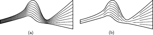
Figure 30.1 Redundancy may occur when surfaces are scan-converted using complete isoparametric curves (a). Adaptive extraction of partial isoparametric curves can produce better result (b).
To proceed in this manner, it is necessary to derive the proper parametric step, σu, so that the two adjacent isoparametric curves will be sufficiently close in Euclidean space. In one approach [27], the isoparametric curves are adaptively spaced using bounds that are derived from the distance function d(v) = f(u + δu, v) - f (u, v). Squared distance d2(t) is represented in the Bézier basis, and its bounds are estimated from its convex hull. A similar technique [18],[25] uses the mean-value theorem. A bound on the Euclidean distance resulting from a small step h in the parametric space of a Bézier curve is computed as ![]() , where n is the degree of C(u), and {Pi} are its control points. Complete isoparametric curves, that span the entire parametric domainof the surface, can then be extracted and scan-converted [27],[25].
, where n is the degree of C(u), and {Pi} are its control points. Complete isoparametric curves, that span the entire parametric domainof the surface, can then be extracted and scan-converted [27],[25].
Using a framework based on complete isoparametric curves, there is no upper bound on the number of times that a single pixel is actually revisited and redrawn. Recall Definition 1 and consider the surface region between two adjacent isoparametric curves in C, with tolerance δ Because C is a valid coverage of S, the two adjacent isoparametric curves should be within distance 2δ. This upper bound of 2δ may be reached at one point (or more) along these two curves while they are arbitrarily close to each other elsewhere. Redundancy, which amounts to visiting the same pixels more than once while scan-converting the curves, is bound to occur. Figure 30.1 (a) shows an extreme case of redundancy resulting from the need to introduce complete isoparametric curves into the surface coverage.
One way to reduce the amount of pixel redundancy in this direct rendering procedure has been introduced by Rappoport [24]. A surface S will be subdivided if the amount of redundancy in S is greater than some acceptable level. The subdivision criterion is based on the range of partial derivatives in the cross direction ∂S/∂v over the patch. As division proceeds and the sub-patches generated become smaller, the range of derivatives across any one patch can also be expected to decrease. If there are significant deviations in the magnitudes of the cross derivatives on the original surface, the whole process may require a large number of subdivisions.
We now present a different approach, following Elber and Cohen [12], that visits and paints all the pixels covered by a surface S, avoiding division but providing a bound on the amount of pixel redundancy in the resulting coverage. Figure 30.1 (b) shows an example of this approach, which adaptively extracts partial isoparametric curve segments and covers the entire surface in an almost optimal way.
Assume that S is in the viewing space. Then the x and y surface coordinates are aligned with the image plane coordinates ix and iy (that is, ix = x and iy = y), and S is the surface after it has been mapped on to the image plane, possibly with a perspective transformation. We are now also ready to introduce a complementary optimality constraint:
Definition 2
A valid coverage of a surface S based on isoparametric curves is considered optimal if the accumulated cost of pixel drawing is minimal over all valid coverages.
A cost function of pixel drawing should take into account the cost of initialization for drawing a curve, amortized over the length of the curve, plus the actual cost of drawing each pixel times the length of the curve in pixels.
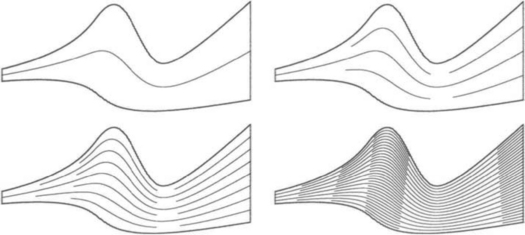
Even if one could compute the required spacing in the parametric domain for a valid coverage of a given surface in a given scene, the extraction of all isoparametric curves in that spacing might be suboptimal, as can be seen from the middle part of the surface in Figure 30.2 (a). Because ∂S/∂v is not constant across the parametric domain of the surface, local dynamic adaptation of the parameter spacing is required, as seen in Figure 30.2 (b), so as to bring the coverage closer to optimal.
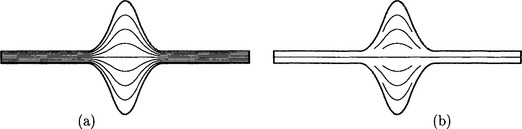
Figure 30.2 Complete isoparametric curves do not provide an optimal valid coverage for this biquadratic B-spline surface (a). Adaptive extraction of isoparametric curves that allows partial curve segments produces a better result and the coverage remains valid (b).
Using isoparametric curves as the coverage for a surface, we define adjacency between two isoparametric curves:
Definition 3
Two isoparametric curves of a surface![]() and
and![]() from a given set C of isoparamet-
from a given set C of isoparamet-
ric curves forming a valid coverage for S, are considered adjacent if, along their common domain![]() there is no other isoparametric curve from C between V1 and v2.
there is no other isoparametric curve from C between V1 and v2.
Now consider two adjacent curves, C1(u) and C2(u). We seek to discover whether the surface region between the two curves, S(u,v), u ∈ U, v1 < v < v2, satisfies the valid coverage constraint within tolerance δ The notion of ‘walking the dog’ is discussed in [1], and named the Frechet metric. The idea is to find the shortest leash that will allow a dog to walk along one curve while its owner walks along the other. If, for C1(u) and C2(u), the leash is shorter than 25, the region between C1(u) and C2(u) is covered, with C1(u) and C2(u) serving as the valid coverage. Unfortunately, the Frechet distance between the two curves is extremely difficult to compute, making its use infeasible in real-time rendering, as such evaluations are required many times for each surface in the scene.
Hence, we employ a much more efficient computational alternative, which bounds the Frechet distance from above; we denote this alternative the iso-distance:
Definition 4
Given two isoparametric curves, C1(u) = S(u,v1) and C2(u) = S(u,v2), their iso-distance function Δ12(u) is defined as![]()
Clearly, the iso-distance between two curves bounds the Frechet distance from above. However, one can find extreme cases where the iso-distance will be arbitrarily large compared to the Frechet distance between the two curves. In section 30.5.1, we will discuss how to deal with such cases.
In generating a rendered image, it is often sufficient to compute the iso-distance using only the x and y coordinate functions of the surface, since our concern is a coverage of the surface in the image plane. For example, consider a planar surface orthogonal to the image plane. This planar surface should be rendered as a line in the image plane: a consideration of iso-distance between isoparametric curves in the planar surface in x and y would indeed yield this result.
Nevertheless, ignoring the z-coordinate in the iso-distance computation may yield a wrong result when the surface is self-occluding or contains silhouette edges when seen from the viewing direction. Hence, for proper rendering using xy iso-distance, the surfaceS should have no silhouette edges, or it must first be split along silhouette edges. Splitting should be conducted once, as a preprocess, creating a set of trimmed surfaces, each of which is free from interior silhouette edges.
In section 30.3.1, we present the adaptive isoparametric curves (AIC) algorithm. In section 30.3.2, we present some examples and discuss the corresponding rendering considerations.
30.3.1 Coverage based on adaptive isoparametric curves
Recall that ![]() are two adjacent isoparametric curves on a surface S. Further, let
are two adjacent isoparametric curves on a surface S. Further, let ![]() . While Δ12(u) is not rational, due to the square root, Δ212(u) is rational. Compare the isodistance square function, Δ212(u), with δ2, where δ2 is the square of the desired tolerance of the coverage (see Definition 1). Several possibilities can occur (note that, for the sake of simplicity, we examine the distances with respect to δ whereas 2δ might suffice):
. While Δ12(u) is not rational, due to the square root, Δ212(u) is rational. Compare the isodistance square function, Δ212(u), with δ2, where δ2 is the square of the desired tolerance of the coverage (see Definition 1). Several possibilities can occur (note that, for the sake of simplicity, we examine the distances with respect to δ whereas 2δ might suffice):
1. ![]() . Here, C1(u) and C2(u) serve as a valid coverage for the region of the surface between the two curves, for v1 ≤ v ≤ v2.
. Here, C1(u) and C2(u) serve as a valid coverage for the region of the surface between the two curves, for v1 ≤ v ≤ v2.
2. ![]() . Here, C1(u) and C2(u) cannot be a valid coverage for the region of the surface between the two curves, for v1 ≤ v ≤ v2. In other words, we must introduce at least one additional, intermediate, curve between C1(u) and C2(u) in order for this set of curves to serve as a valid coverage of the surface region between the two curves, for v1 ≤ v ≤ v2.
. Here, C1(u) and C2(u) cannot be a valid coverage for the region of the surface between the two curves, for v1 ≤ v ≤ v2. In other words, we must introduce at least one additional, intermediate, curve between C1(u) and C2(u) in order for this set of curves to serve as a valid coverage of the surface region between the two curves, for v1 ≤ v ≤ v2.
3. Δ212(u) = δ2 for u = ui, i = 1, ˙ ,n. In other words, the iso-distance function has n locations along the u domain where it is equal to the prescribed tolerance, δ All locations along u where Δ212(u) < δ2 have a valid coverage, using only C1(u) and C2(u), as in Case 1 above. In contrast, for the domain along u for which Δ212(u) > δ2, it is necessary to introduce at least one more intermediate curve between C1(u) and C2(u), as in Case 2 above.
These three cases can be reformulated as a recursive procedure that starts with the two extreme boundary curves of the surface and considers them as two adjacent curves. Then, by examining the equation for the square of the iso-distance between the two curves, one of the three different cases can be identified, leading to two further curves which are dealt with recursively. Algorithm 1 encapsulates the entire process. Line (1) handles the case of two adjacent isoparametric curves that can serve as a valid coverage for the surface region between them. Line (2) considers the case where an intermediate curve must be introduced throughout the shared u domain of the two curves. Finally, in line (3), the final possibility is taken care of, where Δ212(u) intersects the δ2 line; this case further recurses into either Case (1) or Case (2).
There is one other problem. Consider a closed surface, S, where the first and last isoparametric curves, C1(u) and C2(u), of S are identical. In that case, Algorithm 1 would terminate immediately on S. One can always enforce a single subdivision at the top level of the recursion. However, even if the surface is not closed, two different regions might be close to each other, which would raise a similar difficulty. While a completesolution is lacking, in most practical cases δ is far smaller than the surface size and it is highly unlikely that such a failure would occur.
In Figure 30.3, four steps of Algorithm 1 are presented, which demonstrate how these near-optimal coverages are constructed, using segments of isoparametric curves. Clearly, complete optimality cannot be claimed, if only because the iso-distance function is not true distance.
30.3.2 Rendering using adaptive isoparametric curves
Before we can scan-convert the isoparametric curves corresponding to the surface, one must be able to evaluate the normal of the surface at each point of each curve in the coverage. Toward this end, we evaluate the unnormalized surface normal field of S,
where Λ denotes the cross product.
For a bicubic polynomial surface S, the surface normal ![]() (u, v) is a biquintic vector field. For every curve Ci(u) ∈ C that we extract from S, we also extract the normal field curve
(u, v) is a biquintic vector field. For every curve Ci(u) ∈ C that we extract from S, we also extract the normal field curve ![]() i(u) from
i(u) from ![]() (u, v). The quintic normal field
(u, v). The quintic normal field ![]() i(u) is then scan-converted along with the Euclidean curve Ci(u), generating a precise yet unnormalized normal for every pixel. Normalizing the normal field necessitates the evaluation of a square root, which is quite expensive but could be tightly approximated using a lookup table.
i(u) is then scan-converted along with the Euclidean curve Ci(u), generating a precise yet unnormalized normal for every pixel. Normalizing the normal field necessitates the evaluation of a square root, which is quite expensive but could be tightly approximated using a lookup table.
Figure 30.4 shows a simple surface rendered using the AIC coverage. Figure 30.4 (a) shows a rendering in which the iso-distance between two adjacent isoparametric curves is several pixels, while Figure 30.4 (b) shows a similar rendering with a sub-pixel tolerance δ
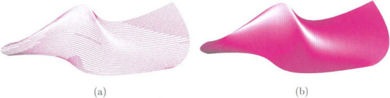
Figure 30.4 In (a), a simple surface is rendered using the AIC-based coverage with a tolerance δ that is several pixels wide. In (b), the same surface is rendered using the AIC-based coverage but with a sub-pixel tolerance Δ
Figure 30.5 (a) shows the Utah teapot scan-converted using traditional polygon rendering methods and Figure 30.5 (b) shows the result based on adaptive isoparametric curves. The highlights that result from the use of the AIC method are superior due to the precise normals that are assigned to each and every pixel. Moreover, using the AIC-based coverage the silhouette curves are clearly smoother. Of course, one could alleviate the artifacts in the highlights and along the silhouette areas in the polygon-based picture in Figure 30.5 (a) by increasing the resolution of the approximation; but then the number of polygons generated could quite easily become very large. The image in Figure 30.5 (a) has a moderate resolution, but even so 7000 polygons were needed to generate it.
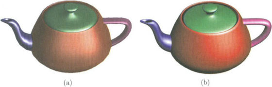
Figure 30.5 In (a), the Utah teapot is rendered using a traditional polygonal approximation, with over 7000 polygons. In (b), the same Utah teapot is rendered using AIC. Note the superior highlights that result, as well as the smoother silhouette edges.
Parametric texture mapping, where the u and v parameters of the surface serve as coordinates into the texture image space, is commonly used in rendering freeform surfaces. By scan-converting isoparametric curves, indexing into the texture image is simplified because one of the surface parameters is fixed, and we are marching along a vertical or a horizontal line of pixels in the texture image. Figure 30.6 (a) shows an example of the Utah teapot with a variety of textures mapped on to it. The body is covered with a parametric texture mapping of the same image applied recursively. The spout, handle, and lid all employ volumetric texture mapping [21],[22] in different patterns: camouflage, wood, and ‘virtual planet’, respectively.
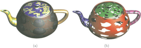
Figure 30.6 In (a), several textures are applied to the Utah teapot. A parametric texture mapping is applied to the body of the pot, with a repeating texture pattern. The spout, handle and cap have all received different volumetric texture patterns. In (b), a set of trimmed surfaces, representing a teapot with holes, are rendered. Both images were created with the aid of an AIC-based coverage of the freeform surfaces.
It is considered difficult to approximate and convert a trimmed surface into polygons for display and rendering purposes [26],[28]. On the other hand, rendering a trimmed surface as a set of isoparametric curves is appealing since the representation of each curve remains
exact after clipping to the domain of the trimmed surface. Because every one of these isoparametric curves is either a vertical or a horizontal line in the parametric domain, clipping itself is relatively straightforward. Figure 30.6 (b) shows another rendering of the Utah teapot, this time with holes formed using trimming curves.
30.4 RAY-TRACING
Methods to ray-trace freeform geometry directly by the numerical evaluation of roots or zero-sets are already known. The demand for extreme robustness and stability (for example, the failure of one pixel in a million would be unacceptable) puts severe restrictions on the possible methods one can use. Some approaches support only special classes of surfaces such as surfaces of revolution, extrusion surfaces and sweep surfaces, or combinations of these. In one such development [4], sweep surfaces are rendered directly, utilizing the generating curves of the sweep surface as the basis for the coverage.
Here, we will examine two approaches that support or emulate direct ray-tracing methods for freeform geometry. In section 30.4.1, we will consider a method that is known as Bézier clipping, which is a robust yet efficient numerical method to derive Ray-Surface Intersections (RSI). In section 30.4.2, we examine an extension to the AIC-based coverage that supports ray-tracing and is called Ruled Tracing.
30.4.1 Bezier clipping
In general, finding the roots of polynomial functions of arbitrary degree is a difficult problem. However, where polynomials represent geometry, the Bézier form may yield some benefits. It should be noted that a B-spline surface can easily be converted to a piecewise Bézier form and hence the method presented here will be equally valid in the domain of B-spline surfaces.
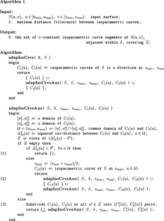
Consider the parametric Bézier curve C(t) = (x(t), y(t)) of degree d. We seek the intersection points of C(t) with the line L : Ax + By + C = 0 (see Figure 30.7 (a)). Substituting C(t) into L, we are left with an implicit equation in one variable whose zero-set corresponds to the desired intersection points, f(t) = Ax(t) + By (t) + C = 0. Clearly, f(t) is a scalar Bézier function of the same degree as C(t),
where Bi,d(t) are Bézier basis functions of degree d. Since the function is scalar, one could replace the coefficients ci by (ci, i/d), in the xy-plane, because ![]() Let us denote the Bézier curve with coefficients Pi = (ci, i/d) as
Let us denote the Bézier curve with coefficients Pi = (ci, i/d) as ![]() 0(t).
0(t).
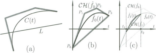
Figure 30.7 In (a), a cubic parametric Bézier curve is to be intersected with line L. The substitution of C(t) into L is shown in (b) as an explicit function ![]() 0(t). Clipping the convex hull domain of
0(t). Clipping the convex hull domain of ![]() 0(t) to be between t1 and t2 results in
0(t) to be between t1 and t2 results in ![]() 1(t), which is shown in (c).
1(t), which is shown in (c).
The curve ![]() 0(t) is contained in the convex hull CH(
0(t) is contained in the convex hull CH(![]() 0) formed by its control points, {Pi}. Moreover, the zeros of f(u) correspond to the intersection points of
0) formed by its control points, {Pi}. Moreover, the zeros of f(u) correspond to the intersection points of ![]() 0(t) with the x-axis. Consider the first control point, P0 of
0(t) with the x-axis. Consider the first control point, P0 of ![]() 0(t) (see Figure 30.7 (b)). If P0 is below the x-axis, as seen in Figure 30.7 (b), then the curve
0(t) (see Figure 30.7 (b)). If P0 is below the x-axis, as seen in Figure 30.7 (b), then the curve ![]() 0(t) is guaranteed to be below the x-axis, as long as CH(
0(t) is guaranteed to be below the x-axis, as long as CH(![]() 0) is also below the x-axis. Similar arguments hold if P0 is above the x-axis. Moreover, the same line of reasoning holds for the last control point, Pd. Hence, one can clip
0) is also below the x-axis. Similar arguments hold if P0 is above the x-axis. Moreover, the same line of reasoning holds for the last control point, Pd. Hence, one can clip ![]() 0(t) from t = 0 up to t1 (see Figure 30.7 (c)), where CH(
0(t) from t = 0 up to t1 (see Figure 30.7 (c)), where CH(![]() 0) intersects the x-axis for the first time, and from t = 1 back down to t2, where CH(
0) intersects the x-axis for the first time, and from t = 1 back down to t2, where CH(![]() 0) intersects the x-axis for the last time, creating
0) intersects the x-axis for the last time, creating ![]() 1(t). The clipped curve
1(t). The clipped curve ![]() 1(t) contains exactly the same zeros as
1(t) contains exactly the same zeros as ![]() 0(t). This numerical process can be allowed to iterate until the zero-set solution is located with sufficient precision.
0(t). This numerical process can be allowed to iterate until the zero-set solution is located with sufficient precision.
The extension of this Bézier clipping process to surfaces requires several intermediate representations, although it follows the general direction of the approach we have taken for curves. Consider the tensor product Bézier surface:
The ray intersecting S(u, v) is defined as the intersection of two orthogonal planes, ![]() Nishita et al. [20] employ the scan plane and the planecontaining the ray and the y-axis are for primary rays. Substitute the control points Pij = (xij, yij, Zij) of S(u, v) into the planes, and let
Nishita et al. [20] employ the scan plane and the planecontaining the ray and the y-axis are for primary rays. Substitute the control points Pij = (xij, yij, Zij) of S(u, v) into the planes, and let ![]() Assuming
Assuming ![]() equals the distance from Pij to the k th plane. We now define a new planar surface as:
equals the distance from Pij to the k th plane. We now define a new planar surface as:
Surface clipping will be conducted over D(u,v), which is merely an orthographic projection of S(u, v) along the ray, if S(u, v) is a polynomial surface. Even if S(u, v) is rational, D(u,v) remains a polynomial.
The solution of D(u, v) = 0 corresponding to the intersection between the ray and the original surface S(u, v) is obtained by performing Bézier clipping steps over D(u, v) with respect to some line in the plane. Nishita et al. [20] give more details and also discuss efficiency and timing considerations. They describe how trimmed surfaces are supported by the manipulation of Bézier trimming curves. Computations of the inclusion/exclusion decisions in both the untrimmed and trimmed domains of the surface are also derived through Bézier clipping. These authors discuss efficiency and timing considerations.
30.4.2 Ruled tracing
At the core of every ray-tracing technique is the need to compute the intersection between a ray R and some surface S, the Ray-Surface Intersection (RSI) problem.
Primary rays are rays from the viewer or the eye through each pixel into the scene; they are typically evaluated in scan-line order, exploiting Z-buffer coherence to solve the RSI problem efficiently. Now consider the problem of casting rays from the points found in primary RSI towards the light sources in the scene, in order to detect regions that are in shadow.
Suppose we have in our scene a horizontal triangular polygon, T, at depth z = 1, positioned above a horizontal rectangular polygon P at depth z = 0 (see Figure 30.8 (a)).
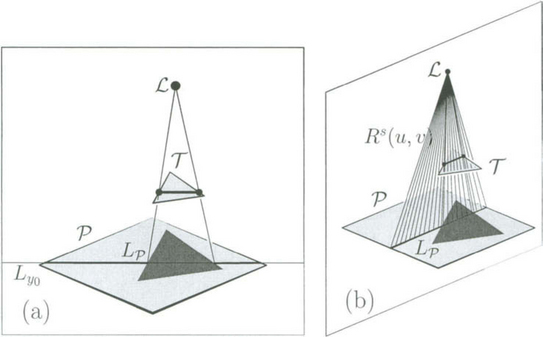
Figure 30.8 In (a), the shadowed regions of P due to T are sought. These regions are then separated from the illuminated domains along the current scan-line, Ly0. In (b), a ruled surface Rs(u, v) is constructed between L and LP, so that Rs(u, v) ∩ T represents the portion of U that is in shadow.
We seek the domain of P in the current scan-line, Lyo, which is hidden from light source L due to T and hence is in shadow. Let ![]() be the domain of P that affects the current scan-line. Traditionally, the domain in shadow along Lp is resolved by emitting one ray per pixel toward L.
be the domain of P that affects the current scan-line. Traditionally, the domain in shadow along Lp is resolved by emitting one ray per pixel toward L.
However, one can approach this shadow detection problem differently. Consider the ruled surface RS that passes through both the light source and the intersecting edge Lp (see Figure 30.8(b)):
We now compute the intersection of Rs(u, v) with the polygon T. If Rs(u, v)∩T is empty, then clearly T casts no shadows on p along the current scan-line Lyo Alternatively, if ![]() , then RS(u0, 0) is hidden from the light source and hence it is in shadow. Moreover, Rs(u0, 0) =LP(u0) and so we have a direct hit on the portion of LP(u) that is in shadow.
, then RS(u0, 0) is hidden from the light source and hence it is in shadow. Moreover, Rs(u0, 0) =LP(u0) and so we have a direct hit on the portion of LP(u) that is in shadow.
Rs(u, v) is a ruled surface, by its construction. In fact, because one of the boundary curves of Rs(u, v) vanishes to a point at L, Rs(u, v) is a developable [8] (and planar) surface. The domain spanned in the u-direction of the set of Rs(u, v) ∩T corresponds to the domain u that is in shadow, or alternatively illuminated, on P for the whole of the current scan-line, Ly0.
In the next section, we take this coherence-based optimization a step further. The objects in the scene are no longer polygons but are now freeform surfaces, and the surface-polygon intersection problem becomes a surface-surface intersection (SSI) problem. In other words, we are about to cast numerous RSI problems into much fewer SSI problems, expressed in the freeform surface domain.
Ruled tracing of freeform surfaces: The AIC elements C that cover a freeform surface S do not have to be scan-line oriented univariate functions or even straight lines. Scan-line oriented rendering requires the intersection of a plane and the surface S(u, v), so as to deal with the primary rays traced back to the eye. Using the AIC coverage, we can entirely eliminate the plane-surface intersections that are needed for conventional scan-line oriented rendering.
The intersection of a plane and a freeform surface S(u, v) is not in general an isoparametric curve. Scan-line oriented rendering incrementally constructs a valid coverage for S(u, v) in the image plane, which guarantees that all pixels in the image plane covered by S(u, v) will be visited. Although scan-line oriented ray-tracing can benefit from ruled tracing, it is possible to eliminate all computation of plane-surface intersections for the primary rays that pass through the eye.
Assume that our scene consists of a set of surfaces S, and recall the AIC coverage C of a freeform surface S. Let Cj be a set of isoparametric curves of Sj(u, v) ∈ S, that forms a valid coverage for Sj(u, v), and let Cij(u) = Sj(u,vi) ∈ Cj. Consider a light source L and define the ruled surface between L and curve Cji(u) as:
Clearly, from its construction, Rsji(u, v) is a generalized cone, or more precisely a developable surface. One of the boundary curves of Rsji(u, v) vanishes to a point, at L. The following observation is fundamental:
If j = k, we are testing for a self-occluding surface. Because the domain of v is open, Cji(u) itself is excluded from this intersection test. That observation allows one to pose a large set of regular RSI problems, millions in a typical image, in term of much fewer developable-surface-surface intersection (DSSI) problems. A solution to the DSSI of Rs(u, v) against all the surfaces in S yields all the RSI solutions necessary to determine the domain of Cji(u) that is in shadow. Hence, one can form a coverage of isoparametric curves Cj for the surface Sj(u, v). Then, for each isoparametric curve Cji(u) ∈ Cj, we resolve its shadow domain by constructing a complete ruled surface from Cji(u) to the light source L. Continuing in this way, we solve the DSSI against all surfaces in the scene.
So far we have shown how to delineate the shadow regions from the illuminated ones. Let V(u) be the unit-size viewing direction toward Cji(u) and let ![]() be the unit-size surface normal along Cji(u) = Sj(u, vi). Let the unnormalized surface normal be denoted by
be the unit-size surface normal along Cji(u) = Sj(u, vi). Let the unnormalized surface normal be denoted by  , with
 ![]() . Then the reflection direction,
. Then the reflection direction, ![]() , can be computed as:
, can be computed as:
Thus, the specular reflection off the univariate domain of Cji(u) is formulated as:
Rrji(u, v) is a ruled surface. Consider the (piecewise) polynomial or rational freeform surface Sj(u, v). Assuming V(u) is (piecewise) rational, then ![]() ji(u) and hence Rrji(u, v) can be represented as (piecewise) rationals. This holds in at least one degenerate case where V(u) is a constant unit vector; namely, the case in which the viewing direction is fixed, which holds for primary rays and for rays originating from light sources at infinity. However, closer inspection of Equation (30.7) reveals that V(u) need not be unit size to generate a rational vector field in the reflection direction (see Elber et al. [13] for more details). Once constructed, Rrji(u, v) is compared against all the surfaces in S, and a ruled-surface-surface intersection (RSSI) is computed between each pair. The colors of the reflections can be determined from these intersections.
ji(u) and hence Rrji(u, v) can be represented as (piecewise) rationals. This holds in at least one degenerate case where V(u) is a constant unit vector; namely, the case in which the viewing direction is fixed, which holds for primary rays and for rays originating from light sources at infinity. However, closer inspection of Equation (30.7) reveals that V(u) need not be unit size to generate a rational vector field in the reflection direction (see Elber et al. [13] for more details). Once constructed, Rrji(u, v) is compared against all the surfaces in S, and a ruled-surface-surface intersection (RSSI) is computed between each pair. The colors of the reflections can be determined from these intersections.
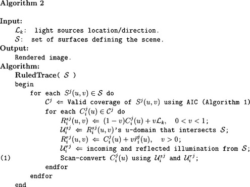
Algorithm 2 summarizes the ruled tracing approach that we have now explained. The algorithm includes computation of the shadowing developable surfaces with respect to the light sources, as well that of the reflecting ruled surfaces, as discussed above. In Line (1) of Algorithm 2, the computation arrives at a single sequence of pixel colors along Cji(u). The term Usi represents the domain of Cji(u) that is in shadow, and Usi expresses the coloring contribution of the reflections along Cji(u), as Rrji(u, v) is intersected against S, based on the colors of the surfaces hit by the reflected ruled surface. In Line (1), the reflectance information and the detected shadows are combined with the original surface properties of Si(u, v) to derive the displayed colors along the entire domain of Cji(u). The next section discusses our implementation and presents some examples, drawing from Algorithm 2.
Examples: Given a ‘black box’ that is able to resolve SSI (surface-surface intersection) queries, the AIC algorithm could be extended to support the emulation of ray-tracing by means of ruled tracing. See Elber et al. [13] for some discussion on specially optimized RSSI (ruled SSI) and DSSI (developable SSI) intersection algorithms.
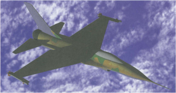
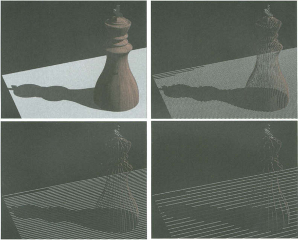
Figure 30.9 shows a computer model of an F16 aircraft, rendered with self-shadowing using ruled tracing. Figure 30.10 shows a king chess piece that was rendered using ruled tracing, with different tolerances in the AIC algorithm.
30.5 EXTENSIONS
The ability to cover a freeform surface using simple primitives has a range of applications and extensions, of which we will consider several here. In section 30.5.1, we will examine the ability to optimize the layout of parametric textures on freeform surfaces which are in general non-isometric. In section 30.5.2, we will apply the AIC coverage to the NC machining of freeform surfaces. Finally, in section 30.5.3, we present line-art rendering techniques of freeform surfaces with the aid of AIC.
30.5.1 Isometric texture mapping
The regular mapping of texture on to parametric surfaces as part of efficient scan-conversion using a set of isoparametric curves is known to be feasible [5],[12],[27]. Unfortunately,
due to the fact that parametric surfaces are rarely isometric, the texture is warped as it is mapped on to the freeform geometry. Attempts to alleviate and control these texture distortions have been made [2],[3],[19] using geodesic curves and relaxation techniques [3],[19] to flatten the surface approximately, or by limiting the viewing directions [2]. In section 30.5.1, we explore the use of the AIC coverage in the search for a less distorted texture mapping.
Texture mapping using AIC: We are interested in the ability to exploit the iso-distance (Definition 4) to produce a minimally distorted texture mapping. While it is clear that the texture will always be distorted for non-developable surfaces, we seek to minimize these distortions.
By accumulating the arc-length of a scan-converted curve as it is traversed, it is possible to know the true distance of any point along the isoparametric curve. Further, the scan-conversion process deals serially with the isoparametric curves in the AIC. Hence, with the aid of Algorithm 1 and the computed iso-distances Δ12(u) we can also accumulate the distance across isoparametric curves.
Measurements of the arc-length of C(u) during the scan-conversion process should be quite accurate. Even so, the (squared) distance represented by Δ122(u) will yield the wrong results if the vectors C1(u)-C2(u) are not orthogonal to ![]() (see Figure 30.11).
(see Figure 30.11).
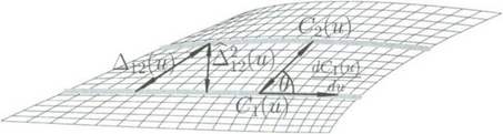
Figure 30.11 The iso-distance as imposed by Δ12(u) could yield wrong results when the vectors C1(u) - C2(u) are not orthogonal to ![]() .
.
Let us denote the angle between vectors C1(u) - C2(u) and ![]() . Then (C1(u) - C2(u)) sin(θ) is a first-order approximation to the true distance between adjacent isoparametriccurves. As the distance between the two adjacent curves converges to zero, the approximation converges to the true distance. Moreover, sin2(θ) can be represented in the following rational form:
. Then (C1(u) - C2(u)) sin(θ) is a first-order approximation to the true distance between adjacent isoparametriccurves. As the distance between the two adjacent curves converges to zero, the approximation converges to the true distance. Moreover, sin2(θ) can be represented in the following rational form:
Then, instead of using Δ212(u), we can employ the more accurate
With these modifications, we can now get a good estimate of distances along, as well as across, isoparametric curves. Nevertheless, it should be noted that nothing is measured nor guaranteed anywhere other than in the tangent plane Tp of the freeform surface. In other words, we are only considering and preserving the ![]() term of the first fundamental form and distance in a direction that is orthogonal to
term of the first fundamental form and distance in a direction that is orthogonal to ![]() in Tp. Clearly, the preservation of these distances does not yield an isometric mapping—as one would indeed expect with general parametric surfaces. Fortunately, in many instances, the parameterization of the surface is well-behaved and the proposed mapping scheme does indeed alleviate the distortions in the resulting texture.
in Tp. Clearly, the preservation of these distances does not yield an isometric mapping—as one would indeed expect with general parametric surfaces. Fortunately, in many instances, the parameterization of the surface is well-behaved and the proposed mapping scheme does indeed alleviate the distortions in the resulting texture.
Distances along and across isoparametric curves are measured and accumulated from one or more prescribed corners of the parametric domain of the freeform surface. While the algorithm can select these corners at random, the final result will change when different corners are used. Hence, the user is given the ability to prescribe the corner or corners from which distances are accumulated. section 30.5.1 demonstrates the effectiveness of this approach using some examples.
Results using AIC texture: Starting with a simple planar yet non-rectangular surface, Figure 30.12 results from the standard texture mapping method as well as from our proposed scheme, with and without the correction of ![]() 212(u), in Equation (30.9).
212(u), in Equation (30.9).
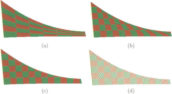
Figure 30.12 A simple planar surface, parametrically texture mapped with red/green checker squares. In (a), traditional texture mapping is exploited using the AIC-based coverage. In (b), the accumulation of arc-length along and across the isoparametric curves is employed. The picture (c) is similar to (a) but with the improved ![]() 212(u) (Equation (30.9)), and (d) shows the same rendering as (c) but with a larger AIC tolerance.
212(u) (Equation (30.9)), and (d) shows the same rendering as (c) but with a larger AIC tolerance.
Finally, in Figure 30.13, a model of an F16 aircraft is rendered using the AIC coverage and almost-isometric mapping. The entire aircraft, except the wings, is rendered using a camouflage-based volumetric texture. In Figure 30.13 (a), checker squares are parametrically mapped on to the wings in the traditional way. In Figure 30.13 (b) the wings of the same F16 are parametrically texture mapped using the distance-preserving scheme presented in this section, yielding an almost isometric texture. Figure 30.13 (c) shows a different texture pattern for the wings.
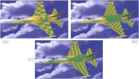
Figure 30.13 A model of an F16 aircraft, with wings that are parametrically texture mapped with a regular pattern. In (a) we see the traditional result that directly follows the (non-isometric) surface parameterization. In (b), almost-isometric texture mapping is employed; and (c) presents a different texture pattern.
More on this almost-isometric texture mapping can be found elsewhere [7].
30.5.2 Machining using adaptive isoparametric curves
Being able to compute the coverage of a surface is a development that holds the key to other problems that require all locations on a surface to be visited to within some prescribed tolerance. An immediate application is Numerically Controlled (NC) machining, in which an AIC coverage can be used to determine a tool path.
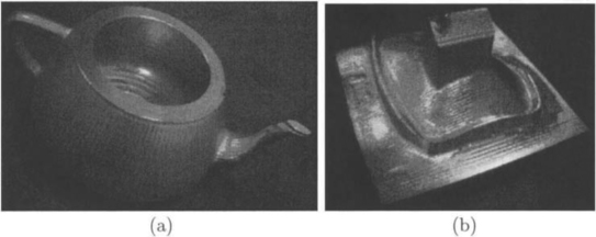
Figure 30.14 shows two examples of freeform shapes that were NC machined using a tool path based on an AIC coverage.
30.5.3 Line-art rendering
Recall the tolerance term δ in Definition 1. So far δ has been assumed to be constant. We will now examine the option of making δ a function. The shading δ(u, v) of a surface can be related to its illumination S(u, v), ∀u, v. In particular, δ can now become a function of the viewing direction and the surface normal, as well as of the position and orientation of the light sources. In pursuit of this goal, we will employ a simple shading model that incorporates both diffuse and specular lighting components [15]. In section 30.5.3, we lay down the necessary background and modifications that are necessary to support δ(u, v), and in section 30.5.3 we present some examples.
Background and modifications towards line-art rendering: In previous work on line-art rendering [29], the Phong lighting model has been employed. We will also use the Phong lighting model in the generation of non-photorealistic line illustrations, this time using the AIC approach. We seek a modification to the surface coverage of Definition 1 so that δ can be employed as a simple shader. Let Li denote the unit vector of the i th light source and let V denote the unit viewing direction. Given a surface S(u, v), let ![]() (u, v) be the unit normal field of S(u, v). Then
(u, v) be the unit normal field of S(u, v). Then
where α is a handle controlling the intensity. The term δ(u, v) in Equation (30.10) prescribes a simple shader with only a diffuse lighting term. Adding a specular term yields
where α and β are handles controlling the different lighting components, and ![]() (u, v) is the direction of light from its source and reflected off S(u, v), expresssed as:
(u, v) is the direction of light from its source and reflected off S(u, v), expresssed as:
(see Equation (30.7)) and c is the power of the specular term. See Foley et al. [15] for more details.
While neither shading model (Equations (30.10) and (30.11)) is (piecewise) rational due to the square-root normalization factors in the unit normal and reflection fields, δ2(u, v) is rational. Because we are actually using δ2(u, v) in our algorithm (see Algorithm 1), the use of the squared function δ2(u, v) imposes no real difficulty.
Unfortunately, results from Algorithm 1 are likely to appear synthetic and artificial due to its binary subdivision nature (see Figure 30.15 (a)). Nevertheless, there exists asimple remedy. One can introduce white noise into the shader, denoted as ![]() (u, v), before solving for the roots of Δ212(u) -
(u, v), before solving for the roots of Δ212(u) - ![]() 2(u, v). This masks the pattern introduced by the binary subdivision: compare Figure 30.15 (a) with Figure 30.15 (b).
2(u, v). This masks the pattern introduced by the binary subdivision: compare Figure 30.15 (a) with Figure 30.15 (b).
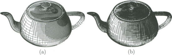
Figure 30.15 The direct adaption of Algorithm 1 to line-art rendering yields results that look synthetic and artificial (a). By adding some random noise to the δ function, these artifacts can be removed (b).
In order to present the results of Algorithm 1 convincingly, it is necessary to eliminate the invisible portion of the coverage. This can be done simply by using a standard Z-buffer to render the freeform surface model so that a complete depth map of the rendered scene is created, using either traditional polygons or the valid AIC coverage rendering that is described in section 30.3.1. Then, the line-art coverage is translated a small distance along the z-direction toward the viewer and its visibility is verified against the depth map, isolating and extracting only the visible portion. This visible portion of the coverage is then approximated using piecewise cubic Bézier curves, which can be represented in the Postscript page description language [23] for printing.
In the next section, we go on to demonstrate some other possibilities of applying the line-art rendering technique to scenes of freeform models.
More examples of line-art rendering: So far we have employed a shader that takes into account both diffuse and specular lighting. We now explore two other possibilities. Consider a shader that enhances silhouette areas,
where ![]() z is the z-component of the unit normal field of surface S(u, v), and c serves as a decay factor as we move away from the silhouettes. See Figure 30.16 (a) for an example.
z is the z-component of the unit normal field of surface S(u, v), and c serves as a decay factor as we move away from the silhouettes. See Figure 30.16 (a) for an example.
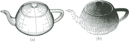
Figure 30.16 The shader can be made to to affect δ(u, v) directly. In (a), this technique is used to enhance silhouette areas, whereas in (b) it is the distance from the light source (above and to the right) that affects δ(u, v).
Yet another possibility is to make the shader respond to the intensity of illumination. The intensity of light decays with the square of the distance from its source; in Figure 30.16 (b), more isoparametric curves are drawn as we get closer to the light, which actually makes the surface look darker!
Further work has been done on the use of AIC for line-art rendering [11]. In addition, attempts have been made to produce drawings of this sort in real time [14].
30.6 CONCLUSION
This chapter has presented several recent results in the direct scan-conversion and ray-tracing of freeform geometry. The ability to cover freeform surfaces optimally and efficiently using primitives which are simple to render, possibly in hardware, has been the key consideration.
In section 30.5.1, we introduced ![]() 212(u) with the aim of improving texture mapping capabilities. It can also be used to give a better AIC coverage, at the expense of more elaborate computations.
212(u) with the aim of improving texture mapping capabilities. It can also be used to give a better AIC coverage, at the expense of more elaborate computations.
The adaptation of the Radiosity rendering scheme to the use of covering curves is more difficult. Isoparametric curves have no area and it is difficult to consider light energy exchange among zero-area elements. While the curves represent a finite surface area with width of the order of δ, direct application of the radiosity method to freeform surfaces remains a topic for research.
In recent years, there has been considerable interest in methods to process and render multivariate functions and surfaces directly. Trivariate functions are extensively exploited in medical visualizations and multivariate functions and surfaces are widely used in scientific visualization. This area of research is also expected to grow in the next few years.
The use of polygons to approximate freeform geometry has many benefits. Nonetheless, this approximation is also deficient in many ways. Recent interest in algorithms for directly handling freeform geometry suggests that the disadvantages of using polygonal approximations become ever more evident, in spite of their extreme simplicity. We will see whether direct surface rendering can challenge their lead.
1. Berlin, Germany, June Alt, H., Godau, M., Measuring the resemblance of polynomial curves. Proc. the 8th Annual Symposium on Computational Geometry. 1992:102–109.
2. N. Arad and G. Elber. Isometric texture mapping. To appear in Computer Graphics Forum.
3. Siggraph, July Bennis, C., Vezien, J.M., Iglesias, G. Piecewise surface flattening for non-distorted texture mapping. Computer Graphics. 1991;25(4):237–246.
4. Bronsvoort, W.F. A surface-scanning algorithm for displaying generalized cylinders. The Visual Computer. 1992;8:162–170.
5. Siggraph, July Catmull, E., Smith, A.R. 3D transformation of images in scanline order. Computer Graphics. 1991;14(3):279–285.
6. Siggraph, July Chang, S., Shantz, M., Rocchetti, R. Rendering cubic curves and surfaces with integer adaptive forward differencing. Computer Graphics. 1989;23(3):157–166.
7. Cohen, E., Elber, G., Minimally distorted parametric texture mapping based on rendering of adaptive isoparametric curves. Proc. the Second “Korea-Israel Bi-National Conference on Computer Modeling and Computer Graphics in the World Wide Web Era”. Seoul, Korea, September. 1999.
8. Docarmo, M.P. Differential Geometry of Curves and Surfaces. Las Vegas: Prentice-Hall; 1976.
9. Siggraph, August Elber, G., Cohen, E. Hidden curve removal for free form surfaces. Computer Graphics. 1990;24(4):95–104.
10. Elber, G. Free Form Surface Analysis Using a Hybrid of Symbolic and Numeric Computation. PhD thesis, University of Utah, Computer Science Department. 1992.
11. September Elber, G. Line art rendering via a coverage of isoparametric curves. IEEE Transactions on Visualization and Computer Graphics. 1995;l(3):231–239.
12. July Elber, G., Cohen, E. Adaptive iso-curves based rendering for free form surfaces. ACM Transactions on Graphics. 1996;15(3):249–263.
13. Elber, G., Choi, J.J., Kim, M.S. Ruled tracing. The Visual Computer. 1997;13:78–94.
14. Milano, Italy, September Elber, G., Interactive line art rendering of freeform surfaces. Eurographics 99. 1999.
15. Foley, J.D., van Dam, A., Feiner, S.K., Hughes, J.F. Fundamentals of Interactive Computer Graphics, Second Edition. Addison-Wesley Publishing Company; 1990.
16. Second Printing Glassner, A.S. An Introduction to Ray Tracing. Academic Press; 1990.
17. Siggraph, July Herzen, B.V., Barr, A.H. Accurate triangulations of deformed, intersecting surfaces. Computer Graphics. 1987;21(4):103–110.
18. Siggraph, July Lien, S., Shantz, M., Pratt, V. Adaptive forward differencing for rendering curves and surfaces. Computer Graphics. 1987;21(4):111–118.
19. September Ma, S.D., Lin, H., Optimal texture mapping. Eurographics 88. 1988:421–428.
20. Siggraph, August Nishita, T., Sederberg, T.W., Kakimoto, M. Ray tracing trimmed rational surface patches. Computer Graphics. 1990;24(4):337–345.
21. Siggraph, July Peachey, D.R. Solid texturing of complex surfaces. Computer Graphics. 1985;19(3):279–286.
22. Siggraph, July Perlin, K. An image synthesizer. Computer Graphics. 1985;19(3):287–296.
23. PostScript Language Reference Manual. Adobe Systems Incorporated, Second Edition. Addison-Wesley Publisher Company: New York, 1994.
24. October Rappoport, A. Rendering curves and surfaces with hybrid subdivision and forward differencing. ACM Transaction on Graphics. 1991;10(4):323–341.
25. August Rockwood, A. A generalized scanning technique for display of parametrically defined surfaces. IEEE Computer Graphics and Applications. 1987;7(8):15–26.
26. Siggraph, July Rockwood, A., Heaton, K., Davis, T. Real-time rendering of trimmed surfaces. Computer Graphics. 1989;23(3):107–117.
27. Siggraph, August Shantz, M., Chang, S. Rendering trimmed NURBS with adaptive forward differencing. Computer Graphics. 1988;22(4):189–198.
28. August Sheng, X., Hirsh, B.E. Triangulation of trimmed surfaces in parametric space. Computer-Aided Design. 1992;24(8):437–444.
29. Siggraph, July Winkenbach, G., Salesin, D.H., Computer-generated pen-and-ink illustration. Computer Graphics. 1994:91–98.