Multiresolution Techniques
The term multiresolution techniques refers to a class of algorithms that decompose a given geometry into its global shape and detail information on different levels of resolution. The representation of an object on several levels of detail which are defined relative to each other gives rise to a number of applications that exploit the hierarchical nature of the representation. In this Chapter we explain the theoretical background of the multiresolution transform and show how the basic concepts can be generalized to arbitrary freeform surfaces.
14.1 INTRODUCTION
One standard approach to facilitate the handling of large amounts of data is to introduce hierarchical structures. Hierarchies usually provide fast access to relevant parts of a dataset which increases the efficiency of any algorithm processing the data. In the context of geometric datasets, hierarchical representations provide, besides spatial decomposition, access to different resolutions of the underlying curve or surface. Depending on the specific application, the term resolution refers to a certain level of complexity or to the amount of geometric detail(cf. Fig. 14.1).

Figure 14.1 For geometric models we distinguish two different types of hierarchies. Topological hierarchies provide different levels of complexity (left) while geometric hierarchies provide different levels of geometric detail information. For spline representations, the link between both hierarchies is established by the basis functions (blending functions) which are associated with the control vertices. For pure polygonal mesh representations there is no canonical way to derive smooth meshes from coarse ones.
If the underlying surface representation is based on splines (cf. chapter 6) or subdivision surfaces (cf. chapter 12) then the topological level of detail characterizes the degree of refinement of the control mesh while the geometric level of detail rates the size of the smallest features and dents on the corresponding continuous surface. If the surface representation is based on polygonal meshes the distinction is more obvious since (topologically) refined meshes can be very smooth (low geometric detail) or highly detailed.
Multiresolution techniques exploit the additional information that becomes available through a level-of-detail (LoD) representation either by choosing an appropriate resolution for given quality (complexity) requirements or by considering the difference between two levels of detail as a separate geometric frequency band which contains the detail information that is added or removed when switching between hierarchy levels.
In this chapter we will first explain the general theoretic set-up for multiresolution representations for curves and surfaces. Based on this formal description we will then discuss specific algorithms and their applications. We will start with the classical representation of a freeform object as a vector-weighted superposition of scalar valued basis functions. Later we generalize this concept to non-nested hierarchies where explicit basis functions are no longer available.
14.2 MULTIRESOLUTION REPRESENTATIONS FOR CURVES
We will introduce the notion of multiresolution analysis and wavelets where we focus on those aspects which are most relevant for geometric modeling applications. For a more detailed exposition we refer to standard books, e.g., [1],[4],[27],[28]
As shown in chapter 6, a standard representation for freeform curves is based on the uniform B-splines
The concept of subdivision curves (chapter 12) has its origin in the observation that the basis function φ satifies a two-scale-relation
which implies the inclusion V = span{φ(˙ - i)} ⊂ V′ = span{φ(2 • -i)}. Consequently we can find a refined representation
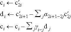
where the new coefficients c′iare computed by the subdivision rules
For B-splines and more general subdivision basis functions we usually have only a finite number of coefficients αi≠ 0. Hence the sum (14.2) only computes a linear combination of a constant number of coefficients ciwhich leads to very efficient subdivision algorithms.
Equation (14.2) defines an identity map from the coarse space V to the fine space V′(with “twice” as many basis functions). Obviously this map is not surjective since V′ contains functions f′which are not in V. Instead of using the basis {φ(2 ˙ -i)} for V′, we try to extend the basis {φ(˙ -i)} by additional basis functions {ψ(˙ - i)} such that
Once we have such a basis function ψ, every function f′∈ V′ can be rewritten as
which can be considered as the reconstruction of the function f′from a coarse scale approximation (defined by the ci) and the detail information (defined by the di).
Since the basis functions ψ(˙ - i) also lie in the space V′, there exists a linear combination which satisfies
and as a consequence we obtain the complete reconstruction rule
In the context of multiresolution transforms, the function φ is usually called the scaling function and ψ is called the wavelet. Both functions are typically designed such that V captures the low frequency component of V′ and W captures the high frequency parts. Depending on the application, additional properties of φ and ψ might be required.
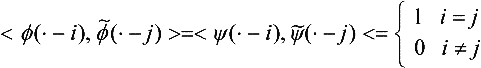
The minimum requirement for this reconstruction to be useful is that for a given function f′we have to be able to efficiently compute well-defined values [ci, di] from the coefficients [c′i]. This inverse reconstruction operation is called the decomposition. For arbitrary basis functions φ and ψ the decomposition requires to solve the linear system defined by (14.3) which is computationally much more expensive than the reconstruction itself. Hence, one tries to balance the computation costs and looks for specific pairs of basis functions ![]() that lead to faster and more effective decomposition operators.
that lead to faster and more effective decomposition operators.
For example, if we can find another set of functions ![]() for which the following conditions hold
for which the following conditions hold
and
then the coefficients ckand dkcan easily be computed by
This setting is called the bi-orthogonal wavelet setting since the conditions (14.4) and (14.5) indicate that the two bases ![]() and
and ![]() are bi-orthogonal (or dual) to each other.
are bi-orthogonal (or dual) to each other.
The reformulation of the decomposition operation in terms of inner products is not necessarily more efficient than solving the linear system directly. However, if we choose special basis functions, the situation simplifies significantly since we do not have to evaluate the inner products by integration.
Assume that there exists a two-scale-relation for the dual basis functions as well
and
then, based on these relations, the inner products reduce to simple linear combinations of control coefficients, e.g.,

and hence
and
respectively. If the dual two-scale-relations have only finitely many non-vanishing coefficients then the decomposition has the same computational complexity as the reconstruction. As we will see in the next section there is a simple technique to construct such pairs of dual refinable basis functions.
Besides the mere applicability of the decomposition, we usually require additional properties of the transform. The obvious requirement is that the coarse approximation fof f′should be as close as possible. Here, the optimal solution can be obtained if we find basis functions ψ(˙ - i) which are orthogonal to the basis functions φ(˙ -i) since in this case the approximation error becomes minimal in the least squares sense. This setting, where V′ = V![]() W is an orthogonal decomposition, is called semi-orthogonal wavelet setting.
W is an orthogonal decomposition, is called semi-orthogonal wavelet setting.
From the theoretical point of view, the optimal representation for a function for f′would be with respect to an orthonormal basis, i.e., not only are the φ(˙ - i) orthogonal to the ψ(˙ -i) but in addition the integer shifts of the basis functions themselves are orthogonal to each other. If this is the case then the dual basis ![]() is identical to the primal one and the magnitude of the coefficients diis proportional to their impact on the shape.
is identical to the primal one and the magnitude of the coefficients diis proportional to their impact on the shape.
Requiring the set [φ(˙ -i), ψ(˙- i)] to be an orthonormal basis is a very strong condition which eliminates most of the degrees of freedom [4]. Additional properties such as smoothness (differentiability), symmetry, and local support of the basis functions φ(˙- i) cannot be satisfied simultaneously anymore. Hence, in many applications, the semi-orthogonal setting is preferred and the additional degrees of freedom are used to obtain smooth basis functions with local support.
However in practice, it often turns out that even the semi-orthogonal setting is quite difficult to establish. Therefore, an even weaker condition is imposed on the basis functions φ(˙ -i) and ψ(˙ - i). The motivation for this weaker condition is that the space V usually contains some low degree polynomials up to order n, i.e.
to guarantee a certain approximation power. Instead of requiring that the basis function ψ(˙- i) be orthogonal to all functions from V we can restrict ourselves to requiring that the basis functions ψ(˙- i) be at least orthogonal to these low degree polynomials
This property is called vanishing moments. For the basis functions ψ(˙- i) to deserve the name “wavelets” we typically have to guarantee at least one vanishing moment (= average function value is zero).
14.3 LIFTING
Lifting [29–31] is a simple technique to construct a set of operators that perform a multiresolution decomposition and reconstruction. The underlying basis functions and their duals correspond to the bi-orthogonal setting and the lifting technique can be used to increase, e.g., the number of vanishing moments of the wavelets.
The starting point for the construction is an arbitrary refinable scaling function φ whose integer shifts φ(˙- i) span a coarse space V. For simplicity we assume that φ is interpolatory, i.e., φ(0) = 1 and φ(i) = 0 for all integers i ≠ 0.
The squeezed basis functions φ(2 ˙ -i) span the refined space V′ and we have V⊂V′ due to the two-scale-relation (14.1).
Suppose we are given a function
in the refined space V′. The simplest way to decompose f′into a coarser approximation
plus detail information
is to apply subsampling to the sequence of coefficients, i.e.,
Applying the subdivision operator (14.2) corresponding to the basis function φ we obtain predicted values
on the refined scale which in general differ from the original values c′2i+1. Hence the detail coefficients dican be defined as the prediction error
Equations (14.8) and (14.9) define the decomposition operator for a multiresolution analysis. The corresponding reconstruction operator is given by
which shows that we implicitly set the detail function ψ to φ(2 ˙ − 1).
The construction so far has all the formal properties that we required. We have a pair of basis functions [φ, ψ] based on which we derive efficient decomposition and reconstruction operators. The dual basis functions never appear explicitly although the coefficients of their two-scale-relations show up in the decomposition rules.
As we mentioned earlier, we would like to have additional properties such as vanishing moments of the wavelet ψ since this guarantees better approximation quality of the original function and consequently smaller detail coefficients.
In the lifting scheme these additional vanishing moments can be obtained by modifying the initial choice for the function ψ. For this we add a linear combination of scaling functions φ(˙ -i), i.e.
where we choose the γjsuch that ψ* has vanishing moments. Obviously γ0 = γ1 = −1/4 and all other γj=0 yield at least one vanishing moment and even two vanishing moments if the function φ is symmetric. More non-zero coefficients γjcan give additional vanishing moments.
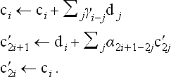
The reason for using the ψ(˙ - i) to enhance the wavelet is that it enables a very simple implementation of the multiresolution transform. For the modified wavelet ψ*we get a new decomposition operator
and the corresponding reconstruction operator is obtained by simply inverting the order of the update steps and changing the signs
Obviously both operators have the same computation cost. Moreover, since the coarse scale coefficients ciand the detail coefficients diare used for mutual updating we can overwrite the old values in each line of the implementation. Hence the whole computation can be done “in place” without using additional memory [31].
The original lifting scheme as proposed by Sweldens [29],[30] is much more general than the construction presented here. In fact, every uniform wavelet transform can be factorized into a number of lifting steps [5]. Moreover, lifting can be applied even in non-uniform settings where the spaces V and V′ are no longer spanned by uniformly spaced shifts of the same basis functions. For more details on the lifting scheme and its usage in different practical applications cf. [31].
14.4 GEOMETRIC SETTING
So far we considered the functional setting, i.e., the geometry was given as the graph of a scalar valued function defined over the real line (or plane). In a more general setup, we have to use parametric representations where the geometry is given by a vector valued function which maps some planar or non-planar parameter domain into 3-space, i.e., each of the coordinates is defined by a separate scalar valued function. As a consequence, control coefficients and detail coefficients are also vector valued.
If we are considering decomposition and reconstruction only then the processing of vector valued functions is done by simply applying the same operators simultaneously to all three coordinate functions. However, if the decomposition is used for multiresolution modeling, i.e., if the position of the control points is changed then a “more geometric” definition of the detail information is necessary.
A typical multiresolution modeling step consists of three stages. First the original geometry is decomposed into global (low frequency) shape and detail information. Then the global shape is modified and finally the detail information is added back by the reconstruction operator. If the detail information is vector valued then the reconstruction will often lead to counter intuitive results since the rotation of the global shape’s tangent is neglected (cf. Fig. 14.2).
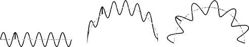
Figure 14.2 If the detail vectors are defined with respect to a global coordinate frame then the reconstruction after a deformation of the global shape (gray line) does lead to artifacts (center). A more intuitive detail preservation is achieved, if the detail is defined with respect to local frames that stay aligned to the global shape.
In order to avoid this effect, Forsey and Bartels [9],[10] introduced the notion of local frame representation of the detail coefficients: Instead of storing the detail vectors diwith respect to some global reference frame F, one rather stores d′i- Fi−1(F(di)) with individual frames Fiwhich depend on the local surface geometry of the low frequency geometry. For example, a local frame that consists of the normal vector and the tangent(s) automatically stays aligned to the underlying curve or surface.
After the modification, the low frequency geometry has changed and hence we find new local frames ![]() . The detail coefficients which are used for the reconstruction are then
. The detail coefficients which are used for the reconstruction are then ![]() ) which guarantees intuitive detail preservation (cf. Fig. 14.2).
) which guarantees intuitive detail preservation (cf. Fig. 14.2).
14.5 MULTIRESOLUTION REPRESENTATIONS FOR SURFACES
The formal description of the multiresolution decomposition and reconstruction so far heavily relies on the regular structure of the control polygon or control mesh. In a regular mesh, all vertices can be labeled by a unique pair of indices, ci,j, and the bivariate subdivision operator computes the new control vertices by
which combines four different averaging rules according to the parity of i and j. The corresponding super- and subsampling operations that are based on the parity of the global indices can only work if the topological neighborhood of each vertex is identical. It is well-known that this requires each inner vertex of a triangle mesh to have exactly six neighbors (or each inner vertex of a quad mesh to have exactly four neighbors). This restriction is too strong for practical modeling applications since the class of possible shapes only contains surfaces which are homeomorphic to (a part of) a torus.
In order to apply multiresolution techniques to more general classes of freeform surfaces we have to extend the concepts of section 14.2 to irregular meshes and non-planar parameter domains, e.g., a closed genus zero surface can be represented as a regular map from the unit sphere into 3-space while there is no regular map from any planar domain.
The standard procedure for finding operators with multiresolution functionality on surfaces with arbitrary topology is to first generalize the sub- and supersampling operations and then define decomposition and reconstruction operators that have properties similar to the original transformations on regular meshes. Ideally the generalized operators coincide with the original ones on regular meshes.
14.5.1 Coarse-to-fine hierarchies
Based on a generalized two-scale-relation, subdivision schemes provide the means to reconstruct a smooth surface from a coarse control mesh with arbitrary topology. The idea is to extend the knot-insertion operation for splines to irregular control meshes. Starting with the initial control mesh M0consisting of the control vertices c01,…,c0n(0), we compute refined control meshes Mmwith control vertices cm1,…,cmn(m) on the m th refinement level. The geometric location of each new control vertex cim+1 is computed by weighted averaging of nearby vertices cmjfrom the unrefined mesh (cf. chapter 12). For triangle meshes we usually have two different types of averaging rules. One for the new vertices cm+1n(m)+1,…,cm+1n(m+1) and one for updating the old vertices cm+11,…,cm+1n(m).
The subdivision operator can serve as the reconstruction operator in a multiresolution representation of a freeform surface. When applying the subdivision operator to a given control mesh Mm, we obtain predicted locations for the control vertices cim+1 on the next level. Detail coefficients dim act like translation vectors which move the vertices back to their original location, i.e., in the reconstruction they undo the prediction error [34]. For the non-functional, geometric setting those displacement vectors have to be encoded with respect to a local coordinate frame (cf. section 14.4).
The multiresolution representation of a surface by subdivision plus displacement on every refinement level mimics most of the important properties that we saw in the previous sections. The displacement vectors dim are local detail coefficients where the length of the vector indicates the significance of the detail and the refinement level on which the displacement is applied indicates the frequency band to which it belongs (cf. Fig. 14.3).
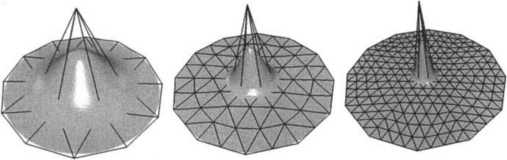
Figure 14.3 The effect of a detail coefficient dim depends on the associated refinement level. The region of the surface that is affected by one detail coefficient corresponds to the support of the basis function associated with the displaced control vertex. Since the support of the basis functions decreases with each refinement step, we obtain a proper decomposition of the geometric shape into different frequency bands.
So far we only considered the reconstruction operator which consists of subdivision plus displacement. For a complete multiresolution functionality we also have to construct a compatible decomposition operator that inverts the reconstruction. The easiest way to obtain such an operator is to apply subsampling to the original mesh Mm+1then apply the subdivision scheme to obtain a mesh M′m+1which is a smoothed version of the original. The detail vectors are found by computing the shift of the vertices caused by this procedure.
Notice that in this case the number of detail coefficients equals the number, n(m+1), of vertices in the fine mesh. This is quite different from the classical wavelet setting where the number of detail coefficients, n(m +1) - n(m), equals the number of vertices that are newly introduced by the reconstruction operator. In principle this does not affect the space and frequency localization properties of the decomposition but it introduces some redundancy since multiple detail coefficients are assigned to the same vertex on different refinement levels. This redundancy can be avoided if we use interpolatory subdivision (cf. chapter 12).
A limitation of the subdivision based multiresolution representation is that it cannot be applied to arbitrary meshes. Because the decomposition is constructed for a prescribed type of reconstruction operator, the subsampling only applies to the special output of that operator. The specific connectivity of the meshes Mm which are generated by the application of a uniform refinement operator is called semi-regular or subdivision connectivity. Semi-regular meshes consist of patches with regular mesh structure and extraordinary vertices (with valence ≠ 6) only occur at the corners of these patches (cf. Fig. 14.4). Meshes to which we want to apply the “inverse subdivision” subsampling have to have this special connectivity.
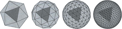
Figure 14.4 Although the base mesh M0can be chosen arbitrarily in the coarse-to-fine setting, the refined resolutions Mm must have subdivision connectivity. This is due to the uniform refinement of the reconstruction operator. The “inverse subdivision” cannot be applied to arbitrary meshes.
We call this type of hierarchy coarse-to-fine hierarchy since the structure of the meshes is determined by the coarsest level M0(which can be arbitrary). All finer meshes Mm are generated by iterative refinement and the decomposition operator only undoes this refinement. If a surface is given by an unstructured triangle mesh which does not have a semi-regular connectivity, remeshing techniques [8],[19],[21] have to be applied which resample the original surface to generate a semi-regular mesh that approximates the original geometry.
The mere displacement of individual control vertices after the refinement corresponds to the initial choice of the wavelet basis function in (14.10). Since the lifting scheme is not restricted to the uniform setting, we can apply it to improve the generalized reconstruction operator in a similar fashion. This leads to more involved reconstruction operators where a detail coefficient associated with one control vertex also affects the position of neighboring control vertices on the same level. Schröder and Sweldens use this technique to design multiresolution decompositions for genus zero surfaces (parameterized over the unit sphere) [26]. Applying the lifting scheme also leads to improved decompositions with non-interpolatory basis functions but does not introduce redundant detail coefficients since the factorization of the transform can be computed in-place.
Another technique to improve the approximation behavior of the decomposition operator is presented in [23]. The construction starts with the nested sequence of spaces Vmwhich are spanned by the subdivision basis functions φim on the m th level (each function φim is associated with the corresponding control vertex cim). On the m th level, the basis φm1,…,φmn(m) is extended to a basis of Vm+1by including the pre-wavelets ![]() . Since the pre-wavelets are related to control vertices from the (m + 1)st refinement level, they are associated with the edges of the mesh Mm.
. Since the pre-wavelets are related to control vertices from the (m + 1)st refinement level, they are associated with the edges of the mesh Mm.
These pre-wavelets are then modified to make them orthogonal to the space Vmsince this guarantees that the decomposition operator finds the best low frequency approximation in the least squares sense (semi-orthogonal setting). The orthogonalization is achieved by subtracting the least squares approximation σim of the function ψim from the space Vm, i.e.,
It turns out that the least squares approximant σim happens to be globally supported in general which means that all si,jare non-vanishing. Since this diminishes the efficiency of the decomposition and reconstruction operator, one tries to find a locally supported approximation of ψim * that is “as orthogonal as possible” to the space Vm. For this one prescribes a support Ωim that is centered around the edge of Mmwhere the vertex cim+1 is going to be inserted. Then one finds the least squares approximation of ψim by using only those basis functions φim whose support lies within the interior of Ωim. By increasing the size of Ωim the resulting basis converges to the semi-orthogonal setting.
14.5.2 Fine-to-coarse hierarchies
The first attempt to generalize the concept of multiresolution representations to freeform surfaces worked from coarse to fine, i.e., we started with the reconstruction operator and the decomposition operator was derived by inverting the reconstruction. The second approach works the opposite way: We start with a decomposition operator building the hierarchy from fine to coarse and then derive the matching reconstruction operator.
The advantage of the fine-to-coarse approach is that it can be applied to arbitrary meshes, no special connectivity is required. The disadvantage is that we no longer have a simple representation of the surface geometry by a superposition of smooth basis functions (as they emerge from subdivision schemes) since the different hierarchy levels are non-nested and hence a proper two-scale-relation cannot be defined.
Given an arbitrary triangle mesh with vertices c1m,…, cn(m)m, we reduce its complexity by applying mesh decimation algorithms, e.g. [2],[11],[14],[17],[22],[25]. Such algorithms remove vertices from the mesh according to some application specific criterion. A typical example for incremental decimation is edge collapsing where one vertex is removed at a time by shifting it into its neighbor’s position and eliminating degenerate triangles (cf. Fig. 14.5).

Figure 14.5 The edge collapse operation reduces the mesh complexity by one vertex and two triangles. Its inverse, the vertex split, can easily be performed if the local neighborhood relations are stored.
This operation reduces the mesh complexity by one vertex and two triangles and can be considered as a basic subsampling step. If we use edge collapsing to remove an independent set of vertices ![]() , i.e., a set of vertices which are not connected by an edge then we achieve a global subsampling which does not require any regularity of the mesh connectivity (cf. Fig. 14.6).
, i.e., a set of vertices which are not connected by an edge then we achieve a global subsampling which does not require any regularity of the mesh connectivity (cf. Fig. 14.6).
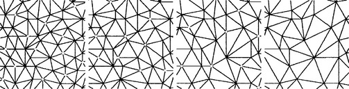
Figure 14.6 Removing an independent set of vertices (hollow dots) from the mesh Mm has the effect of global subsampling but without requiring a regular structure of the mesh connectivity.
The original position of the removed vertices ![]() represents the detail information that is separated from the global shape by the decomposition operation. There are various ways to encode those positions relative to local frames which are aligned to the remaining geometry [20]. The decomposition does not produce redundancy since the number of geometric coefficients (one chunk per vertex) remains constant.
represents the detail information that is separated from the global shape by the decomposition operation. There are various ways to encode those positions relative to local frames which are aligned to the remaining geometry [20]. The decomposition does not produce redundancy since the number of geometric coefficients (one chunk per vertex) remains constant.
Hoppe [14] first observed that the edge collapsing can easily be inverted by vertex split operations. For this we only have to store little extra information about the local connectivity. Hence we immediately find a reconstruction operator which undoes the decomposition. Hoppe used this technique for the progressive transmission of complex meshes by first sending the decimated base mesh to the receiver and then sending a sequence of vertex splits which allow the client to run the mesh decimation backwards until the original model is recovered.
In the context of multiresolution techniques the combination of mesh decimation and progressive refinement yields the necessary pair of basic operators to switch between levels Mm in a multiresolution representation for arbitrary meshes (cf. Fig. 14.7). However, so far we cannot access the smooth low frequency part of the geometry because we cannot refine the mesh without adding back the detail coefficients. For the full multiresolution functionality we have to be able to refine the mesh while suppressing the detail information since otherwise a geometric modification on a coarse scale will not lead to a smooth global deformation of the surface (cf. Fig. 14.8) [18].
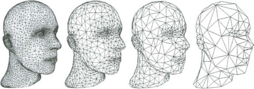
Figure 14.7 A sequence of meshes generated by a mesh decimation algorithm. We can go from left to right by performing edge collapses and we can go from right to left by splitting vertices (progressive meshes).
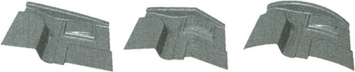
Figure 14.8 A deformation of the global shape is not only characterized by a large support (topologically coarse) but also by its smoothness (low geometric frequency). The object on the left is globally deformed by using a (non-smooth) piecewise linear function in the center and a smooth function on the right.
In the coarse-to-fine setting of the last section the reconstruction without detail is achieved by simply applying the plain subdivision operator without displacement. In the fine to coarse setting, however, we no longer have such smooth basis functions associated with the vertices. As a consequence we have to find a more general prediction scheme that computes the expected position of the new vertices when they are introduced by the supersampling.
The most promissing approaches to generate smooth geometry with unstructured triangle meshes are curvature flow techniques [6],[12],[32] and constrained optimization [16],[18],[24]. Both approaches lead to similar filter algorithms where every vertex of the mesh is shifted to a new position that is computed by a weighted average of its neighbors. The specific weights for these filters are derived from a discrete approximation of some continuous curvature measure and depend on the local connectivity and edge lengths [7].
Based on these techniques we can define the reconstruction operator as follows: Reinsert a subsequence of previously removed vertices ![]() by vertex splits in reverse order. Determine the predicted position of the new vertices by applying a filter operation. Move the vertices to their final position by adding the detail vectors dim
by vertex splits in reverse order. Determine the predicted position of the new vertices by applying a filter operation. Move the vertices to their final position by adding the detail vectors dim
Omitting the last step leads to topologically refined meshes without high frequency detail (cf. Fig. 14.9). If the smoothing filter is applied to the position of the coarse-scale vertices ![]() as well, we can improve the quality of the low frequency geometry but we have to store redundant detail coefficients.
as well, we can improve the quality of the low frequency geometry but we have to store redundant detail coefficients.

Figure 14.9 Starting with the original mesh Mm on the left, we apply mesh decimation to build up a fine-to-coarse hierarchy. The coarsest level M0is shown in the center. When re-inserting the vertices, we can suppress the detail information by computing new (predicted) vertex positions with some smoothing filter. The resulting mesh M′m on the right has the same connectivity as the original mesh Mm but the geometry does not contain any high frequency details.
14.6 APPLICATIONS
Multiresolution representations of geometric models decompose the overall shape into detail information from different scales or frequency bands. These representations are hierarchical in the sense that besides the “horizontal” ordering of the geometric coefficients according to the surface topology (or mesh connectivity) we obtain a “vertical” ordering of the coefficients according to significance or feature size. This vertical ordering is very intuitive since it enables to directly access the shape of an object on various levels of detail.
There are plenty of applications where the augmented structure of hierarchical representations is used to increase the performance by allowing algorithms to focus the processing resources on the significant part of the geometry or by adapting the amount of detail information to the required accuracy. Typical examples for this type of applications are data compression and progressive transmission.
Another class of applications does not rate the detail coefficients according to their significance but tries to exploit the semantic information that emerges from the decomposition. Defining the detail information relative to the global shape is what designers usually do when assembling complex CAD objects. The rationale behind this is that local features are (semantically and physically) attached to the main body of an object and if the main body’s shape is altered then the local features should follow accordingly. The decomposition operator in a multiresolution scheme automatically recovers this type of hierarchical structure from the final shape. While the decomposition cannot identify the functional parts in a CAD model, it can at least distinguish between different feature sizes. Various metaphors for multiresolution editing can be implemented based on this structure.
14.6.1 Multiresolution editing
The general procedure for multiresolution editing is a three step process. First the decomposition operator is applied to separate detail information and global shape. Then the global shape is modified and finally the detail information is added back by the reconstruction operator. The detail reconstruction will be intuitive if the vector valued detail coefficients are encoded with respect to local frames (cf. section 14.4).
For coarse to fine hierarchies, the multiresolution editing is quite simple since we have well-defined subdivision basis functions associated with each control vertex on each refinement level. Early works by Forsey and Bartels [9],[10] already used these technique for hierarchical spline surfaces and Zorin et al. [34] generalized it to subdivision surfaces.
An interesting difference between the two approaches is that for hierarchical splines the control vertices on the different hierarchy levels are considered completely independent while Zorin et al. propagate modifications on the fine levels down to the coarser ones. The goal of this propagation is to keep the detail coefficients on each level as small as possible. Although this makes the reconstruction operator numerically more stable, the strict separation of the detail levels is not preserved.
In [12] Guskov et al. propose a technique for multiresolution decomposition of arbitrary meshes. The decomposition is based on a mesh decimation technique and the reconstruction operator uses a sophisticated smoothing filter for the prediction, i.e., each vertex split during the reconstruction is followed by applying a low-pass filter to a local vicinity. The resulting multiresolution representation is highly redundant since for each vertex split one has to store detail coefficients for all neighboring vertices that are affected by the local smoothing.
One drawback of the above mentioned approaches is that the basis functions which are associated with the mesh vertices are fixed and their definition cannot be adapted to a specific design goal. Therefore in [18] a multiresolution metaphor is presented that builds up the hierarchy on demand. The designer can choose the location and the support of a modification and a fine to coarse hierarchy is then built by applying mesh decimation to the region of the mesh that is covered by the support. Because the resulting decomposition is custom made for one specific editing operation, one does not have to explicitly use the intermediate hierarchy levels but one can restrict to a two-level decomposition (cf. Fig. 14.10).
Figure 14.10 A flexible metaphor for multiresolution edits. On the left, the original mesh is shown. The black line defines the region of the mesh which is subject to the modification. The white line defines the handle geometry which can be moved by the designer. Both boundaries can have an arbitrary shape and hence they can, e.g., be aligned to geometric features in the mesh. The boundary and the handle impose C1 and C0 boundary conditions to the mesh and the smooth version of the original mesh is found by applying discrete fairing while observing these boundary constraints. The center left shows the result of the curvature minimization (the boundary and the handle are interpolated). The geometric difference between the two left meshes is stored as detail information with respect to loacal frames. Now the designer can move the handle polygon and this changes the boundary constraints for the curvature minimization. Hence the discrete fairing generates a modified smooth mesh (center right). Adding the previously stored detail information yields the final result on the right. Since we can apply fast multi-level smoothing when solving the optimization problem, the modified mesh can be updated with several frames per second during the modeling operation. Notice that all four meshes have the same connectivity.
14.6.2 Geometry compression
Techniques for lossy compression of geometry data often exploit the fact that multiresolution decompositions imply an ordering of the detail coefficients according to their significance. If we want to obtain a prescribed compression ratio we can simply remove a certain percentage of the detail coefficients starting with the least significant ones. If we want to stay within a prescribed approximation tolerance, we can remove the least significant detail coefficients as long as we do not violate that tolerance.
Sophisticated multiresolution representations improve the effectiveness of such algorithms. If we choose the right basis functions φ and ψ then the approximation quality of the low frequency component increases and hence the prediction error (= detail coefficients) during the reconstruction becomes smaller. This is the reason why one usually aims at the (approximate) semi-orthogonal setting.
In [23] Lounsbery et al. constructed piecewise linear wavelet functions such that they are, for a given support, as orthogonal as possible to the space of subdivision basis functions. Based on the lifting scheme, Schröder and Sweldens constructed wavelets with vanishing moments for various subdivision schemes and compared their approximation properties [26].
Guskov et al. [13] and Khodakhowski et al. [15] additionally exploit the geometric coherence of a meshed surface by storing the detail coefficients as scalar valued normal displacements instead of vector valued local frame displacements. They achieve this by resampling the orignal geometry such that the tangential component of the displacement vectors vanishes.
All the above multiresolution compression schemes are based on coarse to fine hierarchies. The reason for this is that the availability of subdivision basis functions and their corresponding wavelets allows to adapt the theoretical concepts from the regular functional setting.
In [3] Cohen-Or et al. propose a compression scheme which is based on a fine to coarse hierarchy. Their technique combines ideas from lossless non-hierarchical mesh compression with progressive reconstruction of fine to coarse hierarchies. In every subsampling step they remove an independent set of vertices and retriangulate the resulting holes by triangle strips. In order to keep the detail vectors as small as possible they use a linear prediction scheme that is similar to the low pass filter operations mentioned in section 14.5.2.
Taubin describes a progressive compression scheme in [33]. Here the fine to coarse hierarchy is generated by rather complex “forest splits” which are a generalization of the vertex split operation. The scheme is optimized for connectivity compression.
1. Chui, C. An Introduction to Wavelets. Oxford: Academic Press; 1996.
2. Cignoni, P., Montani, C., Scopigno, R., A comparison of mesh simplification algorithms. Computers & Graphics. 1998:37–54.
3. Cohen-Or, D., Levin, D., Remez, O., Progressive compression of arbitrary triangular meshes. IEEE Visualization Conference Proceedings. 1999:67–72.
4. Daubechies, I., Ten Lectures on Wavelets. CBMS-NSF Regional Conf. Series in Appl. Math, Vol. 61. SIAM: San Diego, 1992.
5. Daubechies, I., Sweldens, W. Factoring Wavelet Transforms into Lifting Steps. J. Fourier Anal. Appl. 1998:245–267.
6. Desbrun, M., Meyer, M., Schröder, P., Barr, A., Implicit fairing of irregular meshes using diffusion, curvature flow. Computer Graphics (SIGGRAPH 99 Proceedings). 1999:317–324.
7. M. Desbrun, M. Meyer, P. Schröder, A. Barr. Discrete Differential-Geometry Operators in nD Preprint.
8. Eck, M., DeRose, T., Duchamp, T., Hoppe, H., Lounsbery, M., Stuetzle, W., Multiresolution analysis of arbitrary meshes. Computer Graphics (SIGGRAPH 95 Proceedings). 1995:173–182.
9. Forsey, D., Bartels, R., Hierarchical B-spline refinement. Computer Graphics (SIGGRAPH 88 Proceedings). 1988:205–212.
10. Forsey, D., Bartels, R., Surface fitting with hierarchical splines. ACM Transactions on Graphics. 1995:134–161.
11. Garland, M., Heckbert, P., Surface simplification using quadric error metrics. Computer Graphics (SIGGRAPH 97 Proceedings). 1997:209–216.
12. Guskov, I., Sweldens, W., Schröder, P., Multiresolution signal processing for meshes. Computer Graphics (SIGGRAPH 99 Proceedings). 1999:325–334.
13. Guskov, I., Vidimce, K., Sweldens, W., Schröder, P., Normal meshes. Computer Graphics (SIGGRAPH 2000 Proceedings). 2000:95–102.
14. Hoppe, H., Progressive meshes. Computer Graphics (SIGGRAPH 96 Proceedings). 1996:99–108.
15. Khodakovsky, A., Schröder, P., Sweldens, W., Progressive geometry compression. Computer Graphics (SIGGRAPH 2000 Proceedings). 2000:271–278.
16. Kobbelt, L. Discrete fairing. In: Proceedings of the Seventh IMA Conference on the Mathematics of Surfaces. Philadelphia, PA: Information Geometers; 1997:101–131.
17. Kobbelt, L., Campagna, S., Seidel, H-P., A general framework for mesh decimation. Graphics Interface Proceedings. 1998:43–50.
18. Kobbelt, L., Campagna, S., Vorsatz, J., Seidel, H.P., Interactive multi-resolution modeling on arbitrary meshes. Computer Graphics (SIGGRAPH 98 Proceedings). 1998:105–114.
19. Kobbelt, L., Vorsatz, J., Labsik, U., Seidel, H-P., A shrink wrapping approach to remeshing polygonal surfaces. Computer Graphics Forum 18. Eurographics ’99 issue. 1999:C119–C130.
20. Kobbelt, L., Vorsatz, J., Seidel, H-P. Multiresolution hierarchies on unstructured triangle meshes. Computational Geometry: Theory and Applications. 1999;14:5–24.
21. Lee, A., Sweldens, W., Schröder, P., Cowsar, L., Dobkin, D., MAPS: multiresolution adaptive parameterization of surfaces. Computer Graphics (SIGGRAPH 98 Proceedings). 1998:95–104.
22. Lindstrom, P., Turk, G., Fast, memory efficient polygonal simplification. IEEE Visualization ’98 Conference Proceedings. 1998:279–286.
23. Lounsbery, M., DeRose, T., Warren, J. Multiresolution analysis for surfaces of arbitrary topological type. ACM Transactions on Graphics. 1997;16(1):34–73.
24. Schneider, R., Kobbelt, L. Geometric fairing of irregular meshes for free-form surface design. Computer Aided Geometric Design. 2001;18(4):359–379.
25. Schroeder, W., Zarge, J., Lorensen, W., Decimation of triangle meshes. Computer Graphics (SIGGRAPH 92 Proceedings). 1992:65–70.
26. Schröder, P., Sweldens, W., Spherical wavelets: efficiently representing functions on the sphere. Computer Graphics (SIGGRAPH 95 Proceedings). 1995:161–172.
27. Stollnitz, E., DeRose, T., Salesin, D. Wavelets for Computer Graphics. Winchester: Morgan Kaufmann Publishers Inc.; 1996.
28. Strang, G., Nguyen, T. Wavelets, Filter Banks. San Franscisco: Wellesley Cambridge Press; 1996.
29. Sweldens, W. The lifting scheme: A custom-design construction of biorthogonal wavelets. Appl. Comput. Harmon. Anal. 1996:186–200.
30. Sweldens, W. The lifting scheme: A construction of second generation wavelets. SIAM J. Math. Anal. 1997:511–546.
31. Sweldens, W., Schröder, P., Building your own wavelets at home. Wavelets in Computer Graphics. ACM SIGGRAPH Course notes. 1996:15–87.
32. Taubin, G., A signal processing approach to fair surface design. Computer Graphics (SIGGRAPH 95 Proceedings). 1995:351–358.
33. Taubin, G., Gueziec, A., Horn, W., Lazarus, F., Progressive forest split compression. Computer Graphics (SIGGRAPH 98 Proceedings). 1998:123–132.
34. Zorin, D., Schröder, P., Sweldens, W., Interactive multiresolution mesh editing. Computer Graphics (SIGGRAPH 97 Proceedings). 1997:259–268.