
Scattered Data Interpolation: Radial Basis and Other Methods
This chapter presents some techniques for solving scattered data interpolation for functional data. The focus here is to present some practical techniques for solving these problems using radial basis functions and some other local methods. Many of these techniques using radial basis functions have been developed only in last few years. Furthermore, although many of these techniques can be extended to higher dimensions, here we concern ourselves mostly with two and three dimensions. For a more comprehensive survey ond literature on scattered data interpolation, we refer the reader to our earlier work [28].
16.1 INTRODUCTION
Scattered data interpolation and approximation problems arise in a variety of applications including meteorology, hydrology, oceanography, computer graphics, computer-aided geometric design, and scientific visualization. There exist several variants of the basic problem. The basic problem, referred to as the functional scattered data problem is to find a surface that interpolates or approximates a finite set of points in a k—dimensional space Rk. Sometimes the scattered data obtained is noisy (for example when collected using a 3D depth range finder) and approximation is desirable. Sometimes the data obtained is fairly accurate (sampled from a given model or an object) and interpolation is desired. In other variations, the data is specified on a sphere or on a surface (such as an aeroplane wing). While all these problems are undoubtedly very interesting, in this work, we focus on the functional scattered data interpolation problem in two or three dimensions.
Solutions to the scattered data interpolation or approximation problem are equally varied. Typically, the researcher makes a-priori choice regarding the type of solutions. Popular choices include polynomial or rational parametric representations, algebraic or implicit representations, subdivision methods, radial basis methods, Shepard’s techniques and a combination of some of these approaches. Although the choice of the type of solution sometimes may be guided by the application domain and the previous methodologies prevalent in the discipline, the distribution of the data points often play an important role in dictating the type of solutions pursued. One of the most important criteria is whether the scattered data is prescribed with an underlying grid or not. When data is uniformly distributed such as in the case of rectilinear or the structured grid (see Figure 16.1), one can employ special types of methods (such as bilinear or trilinear interpolation or more generally non-uniform rational B-splines (NURBS)) that may not be available for truly scattered data. Of course, one can always triangulate scattered data using Delaunay triangulation, for example, and employ methods that take advantages of the underlying triangular grid in two dimensions and tetrahedral grid in three dimensions. This approach has often been used in constructing polynomial or rational parametric and algebraic solutions. In cases where the underlying mesh consists of a mixture of triangles, quadrilaterals, and higher order polygons (or polytopes in higher dimensions), subdivision methods have been applied. Radial basis methods, in contrast, do not assume or need any underlying grid.

Figure 16.1 Different types of grids: regular, rectilinear, structured (each interior data point is connected to exactly four neighbors), unstructured (no restriction on the number of neighbors), scattered (no underlying grid)
Although all of the techniques mentioned above are useful in diverse applications, we have chosen to concentrate on radial basis methods and some local methods in this work. Our choice is guided by the fact that this handbook covers rational parametric solutions and subdivision methods in other chapters. Besides, some exciting recent developments in radial basis methods have made these techniques much more practical for very large data sets that was not possible only a few years ago. Also, we chose to focus on techniques that are likely to be useful in practical applications that often arise without any underlying grids.
16.2 RADIAL INTERPOLATION
We begin by presenting a brief introduction to the radial basis functions. A function φ(rk), where ![]() is referred to as a radial function, because it depends only upon the Euclidean distance between the points (x,y) and (xk,yk). The points (xk,yk) are referred to as centers or knots. In particular, the function φ(rk) is radially symmetric around the center (xk,yk). The solution to the scattered data interpolation problem is obtained by considering a linear combination of the translates of a suitably chosen radial basis function. Sometimes a polynomial term is added to the solution, when φk is conditionally positive definite (defined later in this section), or in order to achieve polynomial precision. More formally, the solution to the interpolation problem is sought in the following form:
is referred to as a radial function, because it depends only upon the Euclidean distance between the points (x,y) and (xk,yk). The points (xk,yk) are referred to as centers or knots. In particular, the function φ(rk) is radially symmetric around the center (xk,yk). The solution to the scattered data interpolation problem is obtained by considering a linear combination of the translates of a suitably chosen radial basis function. Sometimes a polynomial term is added to the solution, when φk is conditionally positive definite (defined later in this section), or in order to achieve polynomial precision. More formally, the solution to the interpolation problem is sought in the following form:
where ql(x,y), l = 1, …, M is any basis for the space Pm of bivariate polynomials of degree less than m, and therefore ![]() . Notice that m = 0, 1, 2 corresponds to the case when no polynomial, constant function or a linear polynomial is added to the interpolant respectively. In order to satisfy the interpolation conditions, one poses the following system of N linear equations in N unknowns Ak, k = 1, …, N, when m = 0:
. Notice that m = 0, 1, 2 corresponds to the case when no polynomial, constant function or a linear polynomial is added to the interpolant respectively. In order to satisfy the interpolation conditions, one poses the following system of N linear equations in N unknowns Ak, k = 1, …, N, when m = 0:
where ![]() is the Euclidean distance between the points (xi, yi) and (xk, yk). When m ≠ 0, a slightly modified system of N + M linear equations in N + M unknowns Ak, k = 1, …, N and Bl, l = 1, …, M is formulated as follows:
is the Euclidean distance between the points (xi, yi) and (xk, yk). When m ≠ 0, a slightly modified system of N + M linear equations in N + M unknowns Ak, k = 1, …, N and Bl, l = 1, …, M is formulated as follows:
In addition, throughout this section we shall assume the following mild geometric condition on the location of scattered data points:
Notice that this geometric condition is vacuous for m = 0, 1. For m = 2, this condition states that all the scattered data points do not lie on a straight line. Assuming that a solution to the system of equations (16.2) or (16.3) exist, the radial basis interpolant is then given by Equation (16.1).
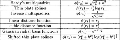
Figure 16.2 presents some examples of radial basis functions with global support, that is, these functions never vanish on any interval. In these examples, h is a parameter. For good choices of this parameter, we refer the reader to [33]. The property of global support poses one of the major practical difficulties in computing and evaluating these radial basis functions. One of the main focuses of this chapter is to present recent developments that address these difficulties and suggest methods of overcoming them. In another approach, radial basis functions with compact support were introduced by several researchers including Schaback, Wu and Wendland [38],[35],[36],[41],[37], and applied to scattered data problems by Floater, Iske and others [17],[24],[18],[26]. However, radial basis functions with compact support seem to exhibit inferior convergence properties in comparison to radial basis functions with global support [13]. Even in the case of radial basis functions with global support, radial basis functions that grow with distances such as multiquadrics and thin plate splines seem to provide superior solutions in many practical applications in comparison to those that decay with distances such as inverse multiquadrics and Gaussian radial basis functions. Therefore, in this work, we focus mostly on multiquadrics and thin plate splines. Surprising though it may seem, these radial basis functions, although not absolute or square integrable, yield very good convergence. The main question, of course, is how to compute and evaluate interpolants using these radial basis functions. Before we turn to this question, we briefly describe some existence and uniqueness properties of these interpolants.
16.2.1 Existence and uniqueness
To describe the existence of radial basis interpolants, we begin with a few definitions. Given a radial function φ(rk) and N scattered data points, consider the N × N square symmetric matrix A = (aij), where aij = φ(rij). The radial function φ(rk) is said to be positive definite iff vt Av ≥ 0 for all v ∈ Rn. The radial function φ(rk) is said to be strictly positive definite if in addition, vt Av > 0 whenever v ≠ 0. If a radial basis function is strictly positive definite, then the matrix A is invertible. This is exactly what is needed in order to solve the system of linear equations (16.2) and guarantee the existence of an interpolant.
However, as mentioned before, for some radial basis functions such as thin plate splines, the matrix A is not always invertible and addition of at least a linear polynomial term to the interpolant is required. To describe these existence results in somewhat greater generality, the notion of conditionally positive definiteness is introduced. Let Pm denote the space of polynomials of degree less than m. Consider the collection V of vectors v = (v1, …, vN) in RN that satisfy ![]() for any q ∈ Pm. The radial function φ(r) is said to be conditionally positive definite (cpd) of order m iff vt Av ≥ 0 for all v ∈ V. The radial function φ(r) is said to be conditionally strictly positive definite (cspd) of order m if in addition, vt Av > 0 whenever v ≠ 0. It can be proved with a little effort that the the system of equations 16.3 is uniquely solvable if the radial basis function is conditionally strictly positive definite of order m and the scattered data points satisfy the geometric condition (16.4).
for any q ∈ Pm. The radial function φ(r) is said to be conditionally positive definite (cpd) of order m iff vt Av ≥ 0 for all v ∈ V. The radial function φ(r) is said to be conditionally strictly positive definite (cspd) of order m if in addition, vt Av > 0 whenever v ≠ 0. It can be proved with a little effort that the the system of equations 16.3 is uniquely solvable if the radial basis function is conditionally strictly positive definite of order m and the scattered data points satisfy the geometric condition (16.4).
Micchelli provided the following characterization for conditionally positive definite functions and derived the following important result:
Theorem: A function f(t) is conditionally positive definite of order m in Rd for d ≥ 1, if and only if ![]() . If in addition
. If in addition ![]() f(√t) ≠ constant, then f(t) is conditionally strictly positive definite of order m.
f(√t) ≠ constant, then f(t) is conditionally strictly positive definite of order m.
It is now easy to verify that multiquadrics (m ≥ 1), inverse multiquadrics (m ≥ 0), thin plate splines (m ≥ 2), linear distance function (m ≥ 1), cubic power of the distance function (m ≥ 2), shifted thin plate splines (m ≥ 2), and Gaussians (m ≥ 0) are cspd of order m up to a constant multiple, that is, either these functions or their negatives are cspd of order m. Some of these results derived from the theorem above can be strengthened further. In particular, the scattered data interpolation problem is solvable with m = 0 and f(t) cspd of order 1, whenever f(t) < 0 for t > 0. This result guarantees the solvability of interpolation problem for multiquadrics without any addition of a constant or a polynomial term. Since so many choices of m are available, what is an appropriate m to choose while using these interpolants? We refer the reader to our previous survey [28] where we have addressed this question along with a number of other issues such as the choice of parameters. We also refer the reader to several articles by Buhmann [13],[12],[11] on radial basis functions. Here, it will suffice to say that in practice, multiquadrics and inverse multiquadrics are implemented without any polynomial term at all or at most with addition of a constant, while the thin plate splines require and are usually implemented with addition of a linear polynomial term.
16.2.2 Computation of the interpolant
The computational cost of direct methods for solving the scattered data interpolation problem using radial basis functions with global support is O(N3), and the storage requirements are O (N2). This is prohibitively expensive even with the fastest workstations currently available. This difficulty has restricted the use of radial basis functions to at most a few thousand centers till recently. However, recent developments may allow fitting data sets up to 5 million data points in 2 dimensions and up to 250,000 points in three dimensions in less than 10 seconds.
There are several approaches that are being actively investigated to compute these interpolants. Here, we present two methods – domain decomposition methods and GMRES (Generalized Minimum Residual) iteration methods [27]. Of these two methods, currently domain decomposition methods are most promising in terms of computing with very large data sets. GMRES iteration methods are less complex to implement and can deal with moderately sized data. Finally, multipole approaches are discussed for evaluating the radial interpolants. We now discuss each of these methods in somewhat greater detail.
Lagrangian and domain decomposition approach
Domain decomposition technique was proposed by Beatson and Powell and further developed by Beatson, Goodsell and Powell for thin plate splines in two dimensions [10],[5]. A proof of convergence for thin plate splines and in fact, for conditionally positive definite radially symmetric functions including multiquadrics, inverse multiquadrics, and Gaussians, for two and higher dimensions was presented by Faul and Powell [16]. Further improvements in the domain decomposition method and numerical results are presented by Beatson, Light and Billings [7].
The domain decomposition method divides the main problem into several small to medium size problems on smaller domains. Lagrange functions are employed on the small and medium size problems. These solutions are then combined to generate an initial approximation to the main problem. An iterative refinement of the initial approximation is performed by computing and improving the residuals.
We now explain each of these steps in somewhat greater detail. A decision is made to divide the main problem into problems of smaller size q, say 30 or 50. A uniformly distributed subset S of the scattered data point of roughly the same size is extracted on which the interpolation problem is uniquely solvable. The remaining points are ordered based on proximity. An initial seed point is chosen to start the ordering. q closest points are then added to this cluster. If there is a tie, it can be broken randomly. One can use alternative methods of structuring decomposing the domain. For example, Beatson, Light, and Billings [7] have used balanced nD-tree to subdivide space into rectangular boxes to guide the decomposition of the space. As we will soon see, Lagrangian interpolations will be performed on clusters of size q.
Now, there are roughly ![]() N/q problems of size q. Let C denote the set of points belonging to one of these smaller subproblems or clusters. On these smaller subproblems, local Lagrange interpolation functions of the following form are used:
N/q problems of size q. Let C denote the set of points belonging to one of these smaller subproblems or clusters. On these smaller subproblems, local Lagrange interpolation functions of the following form are used:
Lagrange functions satisfy the following property: they are exactly 1 at one of the data points and 0 at the remaining q − 1 points, that is, Li(xj) = δij for i, j ∈ C. This yields a system of linear equations. This computation is performed for each of the subproblems once and the results λij are stored for each subproblem. This step is an O(N) process.
The next step is to combine the solutions to these Lagrangian subproblems to generate an initial approximation to the main problem. The initial guess s0(x) starts with zero. For each point in the ordered set (that is for all points except for the points in the subset S), the successive approximant is built as follows:
where,
Please note that the ci(x) is the residual at each point. It can be established that the λii is positive so that the division above does not pose any problems. The main work, therefore, in this algorithm is the computation of the residuals. In the final step of this sweep of the algorithm, the solution σ(x) to the interpolation problem with centers at S with σ(i) = f(i) - s(i) for i ∈ S, is added to complete the first initial approximation to the main problem. Let S1(x) denote the end result after the the first sweep of the algorithm.
Now, an iterative refinement is performed where the entire sweep of the algorithm takes place starting with the initial approximation S1(x). It is remarkable that not only that this algorithm converges, it turns out that there is an increase in accuracy of one digit per sweep of the algorithm, that is, each sweep reduces the maximum error at each data point by a factor of ten, which indicates very fast convergence.
There are several algorithmic and implementation level details that can be incorporated to make this algorithm efficient. For details, we refer the reader to [7]. Numerical results with thin plate splines in two and three dimensions indicate that one can obtain approximately O(N log N) complexity with this algorithm. This allows computation of the interpolant with up to 5 million data points in two dimensions, and up to 250,000 points in three dimensions.
1.1 GMRES iteration
GMRES (Generalized Minimal Residual) algorithm for solving nonsymmetric linear systems was introduced by Saad and Schultz [34]. Implementation of this method using Householder transformations has been discussed by Walker [40]. Beatson, Cherrie and Mouat [4] applied GMRES iteration technique to solve the scattered data interpolation problem using radial basis functions. GMRES iterative methods reduce the computational cost of constructing the interpolant to O(N) storage and O(N log N) operations. The implementation of this method is simpler than the domain decomposition method. Numerical results have been reported using the GMRES method with 10,000 points in two dimensions for thin plate splines and multiquadrics with satisfactory results [4].
As in the domain decomposition method, the GMRES method begins by solving N smaller subsystems of linear equations. Three different strategies have been proposed for constructing these smaller subproblems. These strategies are based on (i) purely local centers, (ii) local centers and special points, and (iii) decay elements. In the purely local centers approach, Lagrange interpolation functions are constructed for the closest points as in the case of domain decomposition method described before. In the local centers and special points approach, some special points uniformly distributed and far away from the local points are added to construct the Lagrange functions in the hope that this will force the deviation of the Lagrange functions to be small near these far away regions. In the decay element approach, the objective is to construct approximate Lagrange functions in the neighborhood of the point and decay rapidly as the distance increases. This is achieved by solving the constrained least squares problem Li(xj) = δij subject to Lj(x) = O(|x|−3) as |x | → ∞. This decay condition is actually equivalent to a homogeneous system of linear constraints. However, decay elements cannot be used exclusively as a basis since they do not span the whole space. Therefore, some non-decay elements are used as well. For some suitable tolerance μ (say, 0.5), the decay element Lij is used if and only if ![]() . Most points in the interior satisfy this criterion. If this condition is not satisfied, then the second method of local centers and special points is used to build the interpolant.
. Most points in the interior satisfy this criterion. If this condition is not satisfied, then the second method of local centers and special points is used to build the interpolant.
The GMRES method differs from the domain decomposition method in how the results of the smaller problems are combined to create an approximate solution to the main problem. Let Lj be the local interpolant associated with the point xj as described in the previous paragraph. Now, we consider the system of linear equations:
where Ψij = Ψj(xi) This system of linear equations is then solved by the standard GMRES technique.
16.2.3 Evaluation
Multipole methods use analytic expansions of the underlying radial functions for large argument, referred to as far-field expansions or Laurent series expansions. The salient ideas for this approach were used by Greengard and Rokhlin [23] to solve numerical integral equations and were applied to the scattered data interpolation problem using radial basis functions by Beatson and Newsam [8].
The overall idea for the evaluation of the interpolant is to break down the evaluation into two parts contributions from the near terms and contributions from the far term. In order to define what is near and what is far, the data is structured hierarchically, for example, using quadtrees. Contributions from the near terms are computed exactly and explicitly. The main challenge is to compute the contributions from the far terms. Contribution from a far term can be approximated well away from the origin by a truncated Laurent series expansion because radial basis functions are analytic at the origin, even when made multivariate through composition with Euclidean norms. However, summing up contributions from each far term using Laurent series expansion is still very costly. The key idea is to form clusters of far terms and combine the Laurent series expansions of each of these clusters into a single Taylor series expansion at the desired point of computation. This method reduces the computation cost to O(1) for each approximate evaluation of the radial interpolant. The accuracy of the computation can be prescribed by the user and can be matched by using appropriate truncation of the series expansions.
Several improvements and extensions of the above algorithm have been proposed in the last decade [6],[9],[3]. In particular, the algorithm described above requires much mathematical analysis of appropriate series expansions and corresponding translator operators for every new radial basis function. Recently, Beatson, Newsam, and Chacko have introduced moment-based methods for evaluating radial basis functions that still take O(1) operations for each single evaluation of the interpolant but in addition, require much simpler implementation to accommodate additional radial basis functions. This is achieved by replacing the far field expansions using Laurent series expansions with computations involving moments of the data.
We now describe each of the steps mentioned above in somewhat greater detail. We first describe the four steps needed to set up the computation. Then we describe the two steps required for the evaluation. In the first step of the set up, the space is subdivided in a hierarchical manner. The space can be enclosed within a given square or a volume. One can then use uniform quadtree subdivisions or adaptive subdivisions depending upon the distribution of the data set. Each subdivided region is referred to as a cell or a panel. Typically, the subdivision is carried down to log N levels. The centers are associated with the cells that they lie in. Two cells are considered near iff they are adjacent to each other. In the next step, far points are to be grouped together. To this purpose, one can define the notion of a distance between two cells based on the hierarchical subdivision of the space using the number of edges in the tree to be traversed to get from one cell to another. Then all the cells that are equidistant from the given cell are grouped together. In the third step, in the original algorithm, Laurent series expansion is computed for eachpoint and translation is used so that these expansions can be reused for other centers. Then these computations are done for each cell starting from the most refined levels or the bottom of the tree and traverse upwards towards coarsers levels forming analogous expressions by combining the computations at the refined levels. In the moment-based algorithms, the moments of the coefficients (used in the solution to the scattered data interpolation problem) around the cell centers are computed from the most-refined levels to the coarser levels of the tree by traversing the tree as before. In the fourth step of the original algorithm, the hierarchical tree is traversed downwards starting from the root and for each cell, Taylor expansion is computed by combining the Laurent series expansions of the whole far field. In the moment-based algorithms, the tree is also traversed downwards as above, however, polynomial approximations are now formed by combining moments and certain approximations to the radial basis functions.
In the evaluation phase, first we identify the leaf node cell (at the bottom of the tree) containing the point where the evaluation is needed. In the second step, the contribution by the near points is computed exactly and precisely. To this we add the contribution by the far points, which is computed by error-driven truncation of the Taylor series expansion of the far fields associated with this cell in the original algorithm or by appropriate evaluation of the polynomial approximations in the moment-based algorithm.
In the moment-based algorithms, real Fast Fourier Transforms (FFTs) are used to compute the required moments. Then the shifted moments corresponding to shifted centers can be computed as convolutions of moments. Computations needed in the approximations of the radial basis functions in the moment-based methods can be greatly reduced by symmetry considerations. Details and some numerical results involving 32000 points in 2D can be found in [3].
16.2.4 Applications
Radial basis functions have been applied in a wide variety of disciplines including bathymetry (ocean depth measurement), topography (altitude measurements), hydrology (rainfall interpolation), surveying, mapping, geophysics, and geology [25]. More recent applications include image warping [42],[1], medical imaging [14], and 3D object representations and reconstructions [15].
Here we discuss some of these applications briefly. In the image warping application by Arad et al. [1], radial basis functions are used to approximate warping of 2D facial expressions. Some key features of the face are identified by a user as pixels or points, referred to as anchor points, on an image. The authors have developed a system for identifying important facial features on eyes and mouth using a technique called generalized symmetry. In the image warping application, an added advantage is that the anchor points need not be specified very accurately. When facial expressions undergo change, new locations of these anchor points are also determined using the feature finding algorithm. This sets up a mapping from R2 to R2 for anchor points. The objective is to find realistic mapping for the whole image. This problem can be decomposed into two independent scattered data interpolation problem from R2 to R. It is well known that if there are only 3 anchor points, one can find an affine mapping from one image to another. In practice, the authors claim that a small number of anchor points yield fairly good results. In examples using the warping of images of Mona Lisa and Ronald Reagan, the authors have used from 6to 14 anchor points. Thin plate splines and Gaussian radial basis functions are used to solve the image warping problem. Thin plate splines have the property that they minimize the bending energy and therefore seem to be appropriate in warping applications. Gaussian radial basis functions can be used to provide a locality condition by judiciously choosing the scalar σ that affects the region of influence around the anchor points. In a variation to the interpolation problem, least squares minimization of the sum of the Euclidean distances between the anchor points is also considered. This variation introduces a scalar factor λ that determines whether the solutions will be a radial solution (when λ = 0) or will be an affine mapping minimizing the least squares distance (when λ = ∞) or somewhere in between. Several results using different values of σ and λ are shown to establish the effectiveness of this approach.
In [14], Carr et al. have used radial basis functions to design cranial implants for the repair of defects, usually holes, in the skull. When a defect is large (≥ 25 sq. cm.), implants are fabricated presurgically. Prefabrication requires an accurate model of the defect area to ensure that a good fit is achieved. Depth maps of the skull’s surface obtained from X-ray CT data using ray-tracing techniques have been used to construct models of cranial defects. The depth map is a mapping from a subset of R2 to R. Due to the presence of defects, the data sets will have holes in the domain. These holes need to be filled. Use of radial basis functions is appealing because no regular underlying grid is available. In this application, a combination of linear radial basis functions and thin plate splines are used. Several examples and results using 300 to 700 points are discussed. Solutions obtained by radial basis functions are compared with the original skull (by artificially introducing holes or defects in the data). Examples for repairing large defects (150 sq. cm.) in convex regions as well as repairing holes close to the orbital margin and other regions of high curvature are also presented.
In the third application, radial basis functions have been used to warp aerial photographs to orthomaps using thin plate splines [42]. Orthomaps, which typically have a pixel resolution of 1 meter on the ground, are produced by a complex and costly process involving acquisition of aerial photographs and ground control data, aerial triangulation, and sophisticated processing of raw images in association with a digital elevation model. However, orthomaps undergo change due to changing characteristics of the region both due to natural (seasonal, wildfires) and man-made changes (new roads, buildings etc.). To update an orthomap, new aerial photographs are taken that need to be registered or warped onto the orthomap because geometric distortions arise in the photographs as a result of the finite height of the aerial camera and the relief of the terrain being imaged. In this application, six image pairs were used for the British Columbia region. This application is very similar to the first one discussed above except that in this case approximately 200 to 300 feature points were selected either manually or using an automated or semi-automated procedure. In this application, aerial photographs were accurate to within 10m on the ground and to within 5m in altitude. Using cross-correlational analysis, the authors concluded that the warped features were corrected with great effectiveness being accurate 50% of the time to within 1.5m, and 90% of the time to within 5m.
16.3 OTHER LOCAL METHODS
Local methods are attractive for very large data sets because the interpolation or approximation at any point can be achieved by considering only a local subset of the data. For data sets of up to at least a few hundred points, global methods such as thin plate splines and multiquadrics are easily applied. Computational experience seems to indicate that for many problems, using very few local points (perhaps fewer than 50 to 100 points) yields surfaces for which the local variations are over-emphasized. This results in what might be described as a somewhat “lumpy” surface, so current recommendation is to take care not to let the surface definition be too locally defined.
Many local methods can be characterized as weighted sums of local approximations, Lk(x,y), where the weights, Wk(x,y) form a partition of unity. Interpolation properties of the local approximations are preserved in the function ![]() provided that each Lk(x, y) takes on the value fj at each (xj, yj) for which Wk(xj, yj) ≠ 0. In order for the overall method to be local, it is necessary that the weight functions be local, that is, nonzero over a limited region, or at a limited number of the data points. We briefly review Shepard methods. These arise from the simple interpolation formula due to Shepard [39] of the form
provided that each Lk(x, y) takes on the value fj at each (xj, yj) for which Wk(xj, yj) ≠ 0. In order for the overall method to be local, it is necessary that the weight functions be local, that is, nonzero over a limited region, or at a limited number of the data points. We briefly review Shepard methods. These arise from the simple interpolation formula due to Shepard [39] of the form  where d2k(x, y) = (x - xk)2 + (y +yk)2 is the square of the distance from (x, y) to (xk, yk) and μ is a parameter, often taken to be 2. This is a global method due to the global weighting functions for the data values. It has well-known shortcomings, such as flat spots at all data points. Many of the shortcomings are overcome by what is called the local quadratic Shepard method, a version of which is available as a Fortran program in the TOMS series, Algorithm 660 [31]. A trivariate version is available as Algorithm 661 [32]. We view the method as a weighted sum of local approximations, where for Shepard’s method, the local approximation Lk(x,y) is fk, and the weight function Wk(x,y) is then clear. We now replace the weight function with another that has compact support and the local approximation with a quadratic function that interpolates the value fk at (xk,yk). The choice for the weight function used by Renka was suggested by Franke and Little [2] and is of the form
 ![]() , where u+ = 0 if u < 0 and u+ = u if u ≥ 0. This weight function behaves essentially like dk(x,y) for (x,y) points near (xk,yk), while becoming zero at distance Rk. The local approximation Lk(x,y) is a quadratic function taking on the value fk at the point (xk,yk) with the other coefficients being determined by a weighted least squares approximation using the data values at a given number of data points near to (xk,yk). The weights for the approximation have the same form as the weight function Wk(x, y) above, but using a different value for the radius at which the weight function becomes zero. Methods such as this can be used easily, with reasonable results. The primary disadvantage for large data sets is that a considerable amount of preprocessing is needed to determine closest points and calculate the local approximations. On the other hand, if approximations are only required in some localized area, the preprocessing may not be burdensome.
, where u+ = 0 if u < 0 and u+ = u if u ≥ 0. This weight function behaves essentially like dk(x,y) for (x,y) points near (xk,yk), while becoming zero at distance Rk. The local approximation Lk(x,y) is a quadratic function taking on the value fk at the point (xk,yk) with the other coefficients being determined by a weighted least squares approximation using the data values at a given number of data points near to (xk,yk). The weights for the approximation have the same form as the weight function Wk(x, y) above, but using a different value for the radius at which the weight function becomes zero. Methods such as this can be used easily, with reasonable results. The primary disadvantage for large data sets is that a considerable amount of preprocessing is needed to determine closest points and calculate the local approximations. On the other hand, if approximations are only required in some localized area, the preprocessing may not be burdensome.
Another version of the weighted local approximation was given by Franke [19]. In this algorithm the search for nearby points and computation of local approximations isenhanced in several ways. The plane is subdivided into a finite rectangular grid, with the goal that each subrectangle contains approximately a specified number of points. The success of this depends on the locations of the data points, and the points may necessarily be poorly apportioned in particular cases. The weight functions are taken to be Hermite bicubic functions with value one and slope zero at the intersection of a vertical and horizontal grid line, and value zero and slope zero at the exterior boundary of the four adjacent subrectangles. This set of functions over the grid points forms a partition of unity. To ensure interpolation it is necessary that the local interpolation function, Wk(x,y) take on the specified value at each of the data points within the four subrectangles adjacent to the corresponding grid point. This approximation is taken to be a thin plate spline, with some accomodation necessary for fewer than the required number of points (that is, three not on a line) within the four subrectangles. While the original paper suggested a fairly small number of points for each set of four subrectangles, later experience indicates the number should be as large as several hundred. The use of rectangular regions greatly simplifies the problem of finding the nonzero terms in the summation since this reduces to a pair of one-dimensional searches to find the subrectangle in which the evaluation point lies. Again, the amount of preprocessing required is substantial. As with the quadratic Shepard method, this can be reduced a great amount if the approximation is to be carried out only in a localized area.
Approximations of the above type can be implemented where the local approximation is determined by least squares, for example. Interpolation will not be maintained, but that may not be an important consideration. One candidate for local approximation in this case is a local least squares multiquadric function. Such functions have been studied by Franke and coauthors [21],[22],[20] and the method appears to be useful using only a small number of knots (centers for the multiquadric basis functions). However, the preprocessing required is greater per local approximation, but this would be offset by a smaller number of local approximations being required. Further, when many evaluations require that it be done rapidly, substantial preprocessing may be acceptable.
Finally, we discuss triangle based methods for solution of the scattered data interpolation problem. The general method we discuss is sometimes described as a finite element method since the approximation is basically a piecewise function defined over a triangulation. We assume that a smooth (continuous first derivatives) interpolation function is to be constructed. For large data sets, the overhead involved in the construction of the triangulation and storage of sufficient information about it may be excessive. This may be overcome in at least two ways. First, we consider methods that use the data points as the vertices of the Delaunay triangulation, and which estimate gradients at the data points from a local subset of the data. Because the Delaunay triangulation is local (made clear by the circle property of the triangulation), it is necessary to process only a subset of the data in the same locality as the evaluation points. Thus the problem can be handled by processing overlapping subsets of the data (some care must be taken to ensure the overlap is sufficient to obtain the same results as for the global problem). Algorithms for performing the triangulation are quite efficient both in terms of time and required computational resources [30]. Once the triangulation is completed (whether only a local part of it, or the global one), the gradients at the vertices need to be estimated. This can be done in a variety of ways, the most successful seeming to be those that fita polynomial approximation to local data points in ways very similar to that described above for the quadratic Shepard method, except here the approximations are only used to obtain gradient estimates. Alternatively, the subset selection method for gradient approximation may be based on the neighbors in the triangulation, and perhaps neighbors of neighbors. This has a certain cohesiveness and also has the advantage of ease of finding the neighbors through the triangulation. On the debit side, points relatively far away could then involved, although generally only near the boundary of the convex hull of the data points.
When the number of data points is excessive, it may be desirable to choose the vertices of the triangulation as a subset of the data points, or to use as vertices other points not directly related to the data points. A procedure for elimination of vertices from a piecewise polynomial approximation of a function was given by Le Méhauté and LaChance [29]. The algorithm eliminates unneeded vertices by calculating a measure of significance for each vertex point, and eliminating those with low significance, subject to maintaining accuracy to within a specified tolerance. The amount of computation for a significant reduction in the number of vertices may be large, but again, may be worthwhile in certain circumstances.
16.4 CONCLUSIONS
Although scattered data interpolation and approximation is a very old problem, new research and recent developments particularly in the area of radial basis functions and subdivision techniques have infused fresh energy into this area. In this work, we have presented a high level view of some of the recent developments that carry great promise for solving practical problems using radial basis functions. This research is still in a state of flux, and many algorithmic and implementation level details need to be stabilized to carve out interpolation and approximation algorithms that can be used by a wider audience. Furthermore, great theoretical advances in radial basis functions have remained inaccessible to the majority of practitioners due to highly sophisticated mathematical presentation of these recent developments. We believe that radial basis function methods are richly deserving of practical implementations for large data sets. We hope that this work provides some pointers to practitioners that will encourage such endeavors.
1. March Arad, N., Dyn, N., Reisfeld, D., Yeshurun, Y. Image warping by radial basis functions: application to facial expressionss. CVGIP: Graphical Models and Image Processing. 1994;56(2):161–172.
2. Barnhill, R.E. Representation and approximation of surfaces. In: Rice J.R., ed. Mathematical Software III. New York: Academic Press; 1977:69–120.
3. Beatson, R.K., Chacko, E. Fast evaluation of radial basis functions: a multivariate momentary evaluation scheme. In: Rabut C., Cohen A., Schumaker L.L., eds. Curve and Surface Fitting. New York: Vanderbilt University Press; 2000:37–46.
4. Beatson, R.K., Cherrie, J.B., Mouat, C.T. Fast fitting of radial basis functions: Methods based on preconditioned GMRES iteration. Advances in Computational Mathematics. 1999;11(2):253–270.
5. Beatson, R.K., Goodsell, G., Powell, M.J.D. On multigrid techniques for thin plate spline interpolation in two dimensions. Lectures in Applied Mathematics. 1996;32:77–97.
6. Beatson, R.K., Light, W.A. Fast evaluation of radial basis functions: methods for two-dimensional polyharmonic splines. IMA Journal of Numerical Analysis. 1997;17(3):343–372.
7. Beatson, R.K., Light, W.A., Billings, S. Fast solution of the radial basis function interpolation equations: domain decomposition methods. SIAM Journal on Scientific Computing. 2000;22(5):1717–1740.
8. Beatson, R.K., Newsam, G.N. Fast evaluation of radial basis functions. Computers and Mathematics with Applications. 1992;24(12):7–19.
9. Beatson, R.K., Newsam, G.N. Fast evaluation of radial basis functions: moment-based methods. SIAM Journal on Scientific Computing. 1998;19(5):1428–1449.
10. Beatson, R.K., Powell, M.J.D. An iterative method for thin plate spline interpolation that employs approximations to lagrange functions. In: Griifiths D.F., Watson G.A., eds. Numerical Analysis. Nashville: Longman Scientific & Technical (Burnt Mill); 1993:17–39.
11. Buhmann, M.D. A new class of radial basis functions with compact support. Tech Report Number 164, Universitat Dortmund, Germany. 1998.
12. Buhmann, M.D. Approximation and interpolation with radial functions. Tech Report Number 169, Universitat Dortmund, Germany. 1999.
13. Buhmann, M.D. Radial basis functions. Acta Numerica. 2000:1–38.
14. February Carr, J.C., Fright, W., Beatson, R.K. Surface interpolation with radial basis functions for medical imaging. IEEE Transactions on Medical Imaging. 1997;16(1):96–107.
15. Carr, J.C., Mitchell, T., Beatson, R., Cherrie, J.B., Fright, W.R., Mccallum, B.C., Evans, T.R. Reconstruction and representation of 3D objects with radial basis functions. In: Fiume Eugene, ed. SIGGRAPH Proceedings. ACM Press; 2001:67–76.
16. Faul, A.C., Powell, M.J.D. Proof of convergence of an iterative technqiue for thin plate spline interpolation in two dimensions. Advances in Computational Mathematics. 1999;11(2):183–192.
17. Floater, M.S., Iske, A. Thinning, inserting, and swapping scattered data. In: Le Mehaute A., Rabut C., Schumaker L.L., eds. Surface Fitting and Multiresolution Methods. Vanderbilt University Press; 1996:139–144.
18. Floater, M.S., Iske, A. Thinning algorithms for scattered data interpolation. BIT. 1998;38(4):705–720.
19. Franke, R. Smooth interpolation of scattered data by local thin plate splines. Computers and Mathematics with Applications. 1982;8:273–281.
20. Franke, R., Hagen, H. Least squares surface fitting using multiquadrics and parametric domain distortion. Computer Aided Geometric Design. 1999;16:177–196.
21. Franke, R., Hagen, H., Nielson, G.M. Least squares surface approximation to scattered data using multiquadric functions. Advances in Computational Mathematics. 1994;2:81–99.
22. Franke, R., Hagen, H., Nielson, G.M. Repeated knots in least squares multiquadric functions. Computing Supplem. 1995;10:177–185.
23. Greengard, L.L., Rokhlin, V. A fast algorithm for particle simulations. Journal of Computational Physics. 1987;73:325–348.
24. Gutzmer, T., Iske, A. Detection of discontinuities in scattered data approximation. Numerical Algorithms. 1997;16(2):155–170.
25. Hardy, R.L. Theory and applications of the multiquadric-biharmonic method. Computers and Mathematics with Applications. 1990;19:163–208.
26. Iske, A. Reconstruction of smooth signals from irregular samples by using radial basisfunction approximation. In: Proceedings of the 1999 International Workshop on Sampling Theory and Applications. Nashville, TN: The Norwegian University of Science and Technology; 1999:82–87.
27. Kelley, C.T. Iterative methods for linear and nonlinear equations. Trondheim: SIAM; 1995.
28. Lodha, S.K., Franke, R. Scattered data techniques for surfaces. In: Nielson G., Hagen H., Post F., eds. Scientific Visualization, Dagstuhl ’97. IEEE Computer Society Press; 1999:181–222.
29. Le Méhauté, A.J.Y., Lachance, Y. A knot removal strategy for scattered data. In: Lyche T., Schumaker L.L., eds. Mathematical Methods in Computer Aided Geometric Design. Academic Press; 1989:419–426.
30. Renka, R.J. Algorithm 624: Triangulation and interpolation of arbitrarily distributed points in the plane. ACM Transactions on Mathematical Software. 1984;10:440–442.
31. Renka, R.J. Qshep2d: Fortran routines implementing the quadratic shepard method for bivariate interpolation of scattered data. ACM Transactions on Mathematical Software. 1988;14:149–150.
32. Renka, R.J. Qshep3d: Fortran routines implementing the quadratic shepard method for trivariate interpolation of scattered data. ACM Transactions on Mathematical Software. 1988;14:151–152.
33. Rippa, S. An algorithm for selecting a good value for the parameter c in radial basisfunction interpolation. Advances in Computational Mathematics. 1999;11(2):193–210.
34. Saad, Y., Schultz, M.H. GMRES:a generalized minimal residual algorithm for solving nonsymmetric linear equations. SIAM Journal of Scientific and Statistical Computing. 1986;7:856–869.
35. R. Schaback. Remarks on meshless local construction of surfaces. In Mathematics of Surfaces X. Oxford University Press. To appear.
36. R. Schaback and H. Wendland. Adaptive greedy techniques for approximate solutions of large RBF systems. Numerical Algorithms. To appear.
37. R. Schaback and H. Wendland. Characterization construction of radial basis functions. In Eilat Proceedings. Cambridge University Press. To appear.
38. Schaback, R., Wendland, H. Numerical techniques based on radial basis functions. In: Cohen A., Rabut C., Schumaker L.L., eds. Curve and Surface Fitting. Vanderbilt University Press; 1999:1–16.
39. Shepard, D., A two dimensional interpolation function for irregular spaced data. Proceedings of 23rd ACM National Conference. 1968:517–524.
40. Walker, H.F. Implementation of the GMRES method using Householder transformations. SIAM Journal of Scientific and Statistical Computing. 1988;9:152–163.
41. Wendland, H. Local polynomial reproduction and moving least suqares approximation. IMA Journal of Numerical Analysis. 2001;21:285–300.
42. Zala, C.A., Barrodale, I. Warping aerial photographs to orthomaps using thin plate splines. Advances in Computational Mathematics. 1999;11(2):211–227.