
Curve and Surface Constructions
This chapter introduces algorithms for the generation of curves and surfaces. The emphasis is on interpolation and approximation using Bézier and B-spline techniques.
7.1 INTRODUCTION
The goal of this chapter is to outline some of the most fundamental interpolation and approximation methods in CAGD. Wherever possible, the developments focus on Bézier and B-spline techniques because of their intuitive geometric definitions. First of all, the focus is on polynomial curve methods, including Lagrange (point) interpolation, point approximation, and Hermite (point and tangent) interpolation. Next, a piecewise polynomial scheme, C2 cubic spline interpolation is presented. The focus then moves to surface methods. The topics include: interpolation to boundary curve data with Coons patches, interpolation to rectangular data with tensor product surfaces, approximation to large sets of data, and interpolation to point and derivative data. Mirroring the curve presentation, a piecewise polynomial surface scheme, C2 bicubic spline interpolation, is discussed. The chapter concludes with volume deformations.
For more information on these topics, a good starting point is one of the following textbooks: [4],[10],[12],[19],[26]. The Bézier Techniques and B-spline Basics chapters 4, 6in this handbook provide an introduction to much of the theory used here.
7.2 POLYNOMIAL CURVE METHODS
Polynomial curve interpolation is a theoretical cornerstone of CAGD. The first topic investigated in this section is the most basic formation of this problem: point data interpolation. Due to its importance, this problem is attacked from three viewpoints, and finally its weakness are examined. Next approximation is examined as a means to overcome the limits of interpolation. This section concludes with point and tangent data interpolation, an important building block for piecewise polynomial schemes.
7.2.1 Point Data Interpolation
Many scientific applications deal with the problem of fitting a curve to discrete point data. In other words, as illustrated in Figure 7.1, given n + 1 data points piwith associated parameters ti, find a degree n polynomial curve p(t) such that
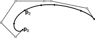
Figure 7.1 Point data interpolation: given n + 1 data points with parameter values, find the interpolating degree n polynomial.
This problem is called point data interpolation.
The ti may be thought of as time increments; they indicate how much time a particle moving along the curve curve must spend between data points. These parameters greatly influence the fitting method, and if their values are not intrinsic to the application, they must be carefully assigned. This topic is addressed in section 7.3.2.
A Direct Approach
Typically, Bézier curves are the preferred representation due to their stability properties (see Farouki and Rajan [13]). Thus the interpolating polynomial with respect to the Bernstein basis takes the form
where the bjare Bézier points and the ![]() (t) are the Bernstein polynomials. The “direct approach” simply means to directly apply the known relationships:
(t) are the Bernstein polynomials. The “direct approach” simply means to directly apply the known relationships:
which are n +1 equations for the n +1 unknowns for each coordinate of the bj. In matrix form:
or p = Bb. The matrix B is called the generalized Vandermonde of the interpolation problem. One can show that the determinant of B is nonzero, and therefore a unique solution to the interpolation problem exists. The direct approach results in two or three (depending on the dimensionality of the data points) linear systems with the same coefficient matrix, therefore it is best to construct the LU decomposition of B.
Instead of using the Bernstein basis, one could choose any basis. The monomials, 1, t, t2,…, tn, have been the historical favorite (see Davis [7]); in this case, the matrix B is simply called the Vandermonde.
Aitken’s Algorithm
If one would simply like to evaluate the interpolating polynomial at specific t parameters, then knowledge of the coefficients of the interpolant is not necessary. Such an evaluation method is Aitken’s algorithm.
The basic idea behind this algorithm is that polynomials may be expressed as linear combinations of lower degree polynomials.1Thus Aitken’s algorithm computes a point on the interpolating polynomial through a sequence of repeated linear interpolations. Given parameter values ti and the data points p0i = pi, compute
Aitken’s algorithm has the following geometric interpretation: priis the result of mapping t with respect to the interval [ti, ti+r] onto the straight line segment through pir-1, pi+1r−1.The geometry of Aitken’s algorithm is illustrated in Figure 7.2for a quadratic example. The intermediate priare computed from two points from the (r − 1)st stage, giving the algorithm, for example for the cubic case, the following structure:
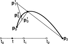
Figure 7.2 Aitken’s algorithm: a point on an interpolating polynomial may be found from repeated linear interpolation.
To prove that Aitken’s algorithm (7.2) interpolates, suppose that the following two interpolation problems have been solved.
Aitken’s algorithm defines the final interpolant as
Figure 7.3illustrates this form for a cubic example. One needs to verify that (7.4) does in fact interpolate to all given data points pi. For t = t0interpolation holds:
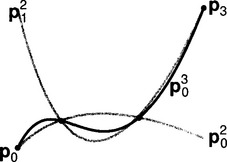
Figure 7.3 Polynomial interpolation: a cubic interpolating polynomial may be obtained as a “blend” of two quadratic interpolants.
A similar result is derived for t = tn. The initial assumption was that p0n−1(ti) = p1n-1(ti) = pifor all other values of i, thus since the weights in (7.4) sum to one identically, pn0o(ti) = pi.
One can infer several properties of the interpolating polynomial from Aitken’s algorithm:
• Affine invariance: this follows since Aitken’s algorithm uses only barycentric combinations.
• Linear precision: If all piare uniformly distributed2on a straight line segment, all intermediate pri(t) are identical for r > 0. Thus the straight line segment is reproduced.
• No convex hull property: the parameter t in (7.2) does not have to lie between tiand ti+r. Therefore, Aitken’s algorithm does not use convex combinations only: pn0(t) is not guaranteed to lie within the convex hull of the pi. One should note, however, that no smooth curve interpolation scheme exists that has the convex hull property.
• No variation diminishing property: if a straight line intersects the polygon connecting the data points m times, then the line can intersect the curve more than m times. In other words, the curve wiggles more than the polygon. This follows for the same reason there is no convex hull property.
The Cardinal Form
The cardinal form of a curve or surface representation is the one in which the given data appear explicitly. With regard to our interpolation problem, the cardinal form would take the form
The basis functions ![]() (t) can be defined by examining the properties which they must posses. Of course they must sum to one in order for (7.5) to be a barycentric combination. Additionally, the
(t) can be defined by examining the properties which they must posses. Of course they must sum to one in order for (7.5) to be a barycentric combination. Additionally, the ![]() (t) must satisfy
(t) must satisfy
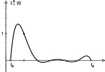
with δi,jbeing the Kronecker delta. In other words, the ith Lagrange polynomial vanishes at all knots except at the ith one, where it assumes the value 1. From this information, one can conclude that the Lagrange polynomials ![]() take the form
take the form
Figure 7.4illustrates one such polynomial over a particular knot sequence.
The cardinal form is primarily used for theoretical analysis. In particular, the Lagrange polynomials are useful in answering the following questions:
The interpolant in (7.5) is the only representation in which the data appear explicitly. Therefore, it is often referred to as the interpolating polynomial or the Lagrange interpolant even though it could be written it in another basis, as illustrated in section 7.2.1
Asking Too Much of a Polynomial
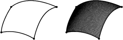
In practical curve fitting scenarios, it is likely that the number of data points exceeds ten. As the number of points increases, the main drawback of polynomial interpolation becomes apparent, as illustrated in Figure 7.5: polynomial interpolants may oscillate. The left curve in that figure is the Lagrange interpolant to 21 points read off a quarter of an ellipse. The data points were computed to a precision of six digits. Slightly changing the input data points, namely by reducing their accuracy to four digits, produces the right interpolant. This is a disturbing phenomenon: minuscule changes in the input data may result in serious changes of the result. Processes with that behavior are called ill-conditioned.
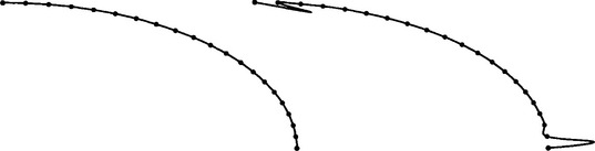
Figure 7.5 Lagrange interpolation: The left and right input data only differ by the amount of accuracy: six digits after the decimal point, left; four digits, right.
This tendency of polynomial interpolants to oscillate has been studied extensively in numerical analysis, where it is known as the “Runge phenomenon” [27]. Sample a small number of points and parameter values from a smooth curve for interpolation, and then gradually increase the number of points. One would expect the interpolant to converge to the underlying, smooth curve, however, this is not the case in general. For some sampled curves, the interpolant diverges. This phenomenon is not due to numerical effects; it is actually inherent in the polynomial interpolation process. An interesting observation is that this does not contradict the Weierstrass approximation theorem.
7.2.2 Point Data Approximation
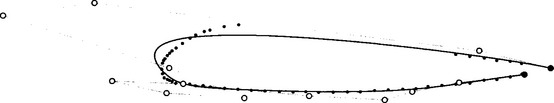
The oscillatory nature of high degree polynomial interpolation, as discussed in section 7.2.1, prompts one to search for a better solution. Approximation of given data by a low degree curve which passes “close” to the data points is a practical solution, as illustrated by Figure 7.6. The added benefit of approximation is a smoothing effect: this is favorable if an application produces data points which are noisy. The first step in building an approximation scheme is to consider a metric to measure closeness. Also, the method should produce a unique solution once given such a metric.

Figure 7.6 Least squares approximation: data points are sampled from the cross section of an airplane wing and a quintic Bézier curve is fitted to them.
Least squares approximation is the most widely used approximation method; it is simple to employ and it uses a familiar metric. The given information consists of m + 1 data points piwith associated parameter values ti. Find a degree n polynomial psuch that the squared distances ||pi- p(ti)||2 are minimal. To make this more concrete, suppose that pis a Bézier curve, thus find the bjwhich minmize the function
The minimization of f may be done componentwise, thus with a slight abuse of notation, formulate the n + 1 equations (for each component) as
After differentiating, these n + 1 equations take the form
and are referred to as the normal equations.
Alternatively, one may formulate the approximation problem similarly to the direct approach from section 7.2.1. Simply write down the given conditions!
This may be condensed into matrix form:
Assuming the number of data points, m +1, is larger than the degree n of the curve, this linear system is overdetermined. One may simply multiply both sides by MT:
This is a linear system with n + 1 equations in n + 1 unknowns with a square and symmetric coefficient matrix MTM. The Bni are assumed to be linearly independent, thus the n + 1 columns of M are linearly independent, and this ensures full rank of MTM. Notice that (7.10) is identical to (7.8), thus this solution also minimizes the L2 norm.
This direct approach for constructing an approximation allows for an additional approximation tool. It may be the case that even the least squares approximation produces a curve that wiggles too much, as illustrated in Figure 7.7. Another defect of the solution in this figure is the wildness of the control polygon. One benefit of the Bézier method is that the polygon often times is a good approximation of the curve’s shape. To achieve this, one could impose restrictions on the control polygon, for example minimize the wiggles in the second differences:
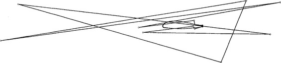
Figure 7.7 Least squares approximation: a degree 13 Bézier curve fitted to the airplane wing data set.
which may be abbreviate as
Simply add these equations to the overdetermined system (7.9),
The factor α (restricted to [0, 1)) gives control over the influence of the added equations. It is solved in the same way as (7.9), that is, by forming the symmetric linear system of normal equations. The system is solvable because the coefficient matrix of (7.12) still has n +1 linearly independent columns, as inherited from the initial matrix M.
The airplane wing data for Figure 7.8was created by decimating the data from Figure 7.6. A simple least squares solution (7.9) to this data would produce a polygon that looks worse than that of Figure 7.7. However, by employing shape equations, here with α = 0.1, results in the solution shown.
7.2.3 Point and Tangent Data Interpolation
Lagrange interpolation can wiggle unexpectedly, thus in an effort to gain more control, one may specify tangents at the data points. Then the given information consists of points pi, associated parameter values ti, and associated tangent vectors mi. Interpolating to this data, a cubic polynomial is constructed between each piand pi+1. This is called cubic Hermite interpolation.Figure 7.9illustrates the result of cubic Hermite interpolation over several segments. Since adjacent segments share the same tangent vector, a globally C1 interpolant is the result.
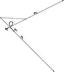
Figure 7.9 Cubic Hermite interpolation: the given point, tangent, and parameter data together with an interpolating cubic in Bézier form.
Consider the two points p0, p1, two tangent vectors m0, m1, and parameters t0and t1. The objective is to find a cubic polynomial curve p(t) that interpolates to these data:
where the dot denotes differentiation. The interpolant pwill be written in cubic Bézier form, and therefore it is left to determine the four Bézier points, two of them are quickly determined:
The endpoint derivatives for Bézier curves are
where Δt = t1- t0. Thus we can easily solve for b1and b2:
Thus the interpolant in Bézier form takes the form
for the global parameter t ∈ [t0, t1] and the local parameter ![]() , which lies in [0,1].
, which lies in [0,1].
The cardinal form of the interpolation problem is characterized by the given data appearing explicitly in the equation for the interpolant. Simply rearrange (7.13):
where

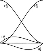
The ![]() are called cubic Hermite polynomials and are shown in Figure 7.10. An additional requirement for the
are called cubic Hermite polynomials and are shown in Figure 7.10. An additional requirement for the ![]() to be cardinal functions for the cubic Hermite interpolation problem is the following: They must be cardinal with respect to evaluation and differentiation at t = t0and t = t1, which means that each of the
to be cardinal functions for the cubic Hermite interpolation problem is the following: They must be cardinal with respect to evaluation and differentiation at t = t0and t = t1, which means that each of the ![]() equals 1 for one of these four operations and is zero for the remaining three. Another property to note is that the point coefficients must sum to one if (7.14) is to be geometrically meaningful:
equals 1 for one of these four operations and is zero for the remaining three. Another property to note is that the point coefficients must sum to one if (7.14) is to be geometrically meaningful: ![]() (t) +
(t) + ![]() (t) ≡ 1. This is of course also verified by inspection of (7.15).
(t) ≡ 1. This is of course also verified by inspection of (7.15).
7.3 C2 CUBIC SPLINE INTERPOLATION
C2 cubic spline interpolation is probably the most frequently used application of B-splines. The problem statement is as follows:
Given: a set of data points p0, …, pKand a knot sequence τ0, …, τK and a knot multiplicity vector 3, 1, 1, …, 1, 1, 3.
Find: a set of B-spline control points d0, …, dLwith L = K +2 such that the resulting C2 piecewise cubic curve x(u) satisfies
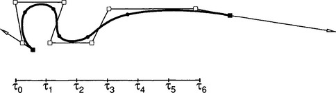
Consult Figure 7.11for an example of the numbering scheme. The triple end knots force the curve to interpolate to the first and last data point:
thus equations for d0and dLmay be eliminated from the list of unknowns. Even so, the above problem is underdetermined because the number of unknowns is K + 1, whereas the number of given data points is K − 1. Typically two end conditions are specified in order to have a uniquely solvable problem. To begin with, consider clamped end conditions; other end condition are presented in section 7.3.1. A clamped end condition corresponds to the prescription of two derivatives ![]() (τ0) and
(τ0) and ![]() (τK),
(τK),
The clamped end conditions yield
therefore equations for d1and dL−1may be eliminated from the list of unknowns also. With end point interpolation and clamped end conditions, the first and last equation of the linear system are
with
Because of the local support property of cubic B-splines, each of the remaining unknowns d2, …, dL−2is related to the data points by
Together, these are K -1 equations for the K − 1 unknown control points. In matrix form, these equations take the form
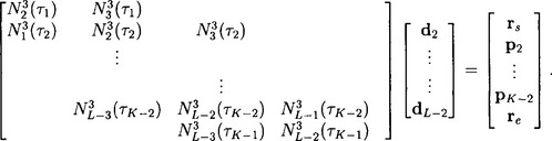
Schematically, the case K = 5 looks like this:
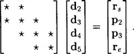
The entries in this tridiagonal matrix are easily computed from the definitions of the cubic B-splines ![]() . In the case of uniform knots ui = i, the interpolation conditions (7.17) take on a particularly simple form:
. In the case of uniform knots ui = i, the interpolation conditions (7.17) take on a particularly simple form:
7.3.1 End Conditions
For C2 cubic spline interpolation, the choice of end conditions is important for the shape of the interpolant near the endpoints. Clamped end conditions, as employed in the previous section, are intended to be used in situations where the end derivatives are actually known. But in most applications, one does not have this knowledge. Still, two extra equations are needed in addition to the basic interpolation conditions (7.16). Below is a list several other end condition methods.
Natural end conditions are derived from the physical analogy of a wooden beam which is clamped at some positions. Beyond the first and last clamps, such a beam assumes the shape of a straight line. A line is characterized by having a zero second derivative, and hence the end conditions
are called “natural” end conditions. In terms of B-spline control vertices (using triple end knots), this becomes
where Δi = τi+1- τi. Rearrange this equation for the linear system and obtain
A similar condition holds at the other endpoint. Unless required by a specific application, this end condition should be avoided as it forces the curve to behave linearly near the endpoints.
Bessel end conditions typically yield better results than natural end conditions. They are defined as follows: the first three data points and their parameter values determine an interpolating quadratic curve. Its first derivative at p0is taken to be the one for the spline curve. This results in
This value for d1is then used in the clamped end condition in the previous section. The control point dL−1is obtained in complete analogy; it is then also used for a clamped end condition.
Quadratic end conditions require ![]() . If all data points and parameter values were read off from a quadratic curve, then this condition would ensure that the spline interpolant reproduces that quadratic. The same is true, of course, for Bessel end conditions.
. If all data points and parameter values were read off from a quadratic curve, then this condition would ensure that the spline interpolant reproduces that quadratic. The same is true, of course, for Bessel end conditions.
Not-a-knot end conditions work from the premise that if the first and second cubic segment are parts of one cubic, then their third derivatives at τ1would agree. The name is derived from the fact that the knot τ1does not act as a breakpoint between two distinct cubic segments.
7.3.2 Defining a Knot Sequence
The spline interpolation problem almost always assumes that parameter values τiare given along with the data points pi. These parameters dictate the amount of time an imaginary particle on the curve spends between piand pi+1relative to the neighboring curve segments. If the data points are not derived from a time dependent application, then just how to assign parameter values is not entirely intuitive, yet their choice can have a significant influence upon the shape of the resulting interpolant.
The easiest way to determine the τiis simply to set τi = i. This is called uniform or equidistant parametrization. This method is too simplistic to cope with most practical situations because it “ignores” the geometry of the data points by spending the same amount of time between any two adjacent data points. Drastic changes in spacing of the data can result in overshooting of the interpolant.
The chord length parametrization is a simple method which is a great improvement over the uniform parametrization. The knot spacing is proportional to the distances of the data points:
where Δi = τi+1- τi. Equation (7.21) does not uniquely define a knot sequence; rather, it defines a whole family of parametrizations that are related to each other by affine parameter transformations.
The centripetal parametrization [20] improves upon the chord length idea. If one sets
the resulting motion of a point on the curve will “smooth out” variations in the centripetal force acting on it.
The uniform parametrization is the only one that is invariant under affine transformations of the data points. All other methods involve length measurements, and lengths are not preserved under affine maps. One solution to this dilemma is the introduction of a modified length measure, as described in Nielson [24]. For more literature on parametrizations, see [6],[9],[15],[17],[18],[25]. There is probably no “best” parametrization, since any method can be defeated by a suitably chosen data set.
7.3.3 The Minimum Property
In the early days of design, a smooth curve was manually drawn through a given set of points by placing metal weights, called “ducks,” at the data points, and then passing a thin, elastic wooden beam, a “spline,” between the ducks. The resulting curve is always very smooth and usually aesthetically pleasing. The wooden beam assumes a position that minimizes its bending energy. The mathematical model of the beam is a curve x(u), and its bending energy E is given by
where κ denotes the curvature of the curve, ds is the arc length of the beam, l is the length of the beam, and c is a constant determined by the material of the beam.
The integral of the curvature of most curves is difficult to work with, therefore for mathematical simplicity, one often approximates the above integral by a simpler one:
Note that Êis a vector; it is obtained by performing the integration on each component of x. The penalty for mathematical simplicity is accuracy. The curvature of a curve is given by
But it must be that ![]()
![]() 1 in order for
1 in order for ![]() to be a good approximation to κ. This means, however, that the curve must be parametrized according to arc length. This assumption is not very realistic for cubic splines in a design environment.
to be a good approximation to κ. This means, however, that the curve must be parametrized according to arc length. This assumption is not very realistic for cubic splines in a design environment.
While the classical spline curve merely minimizes an approximation to (7.23), methods have been developed that produce interpolants which minimize the true energy, see [22], [5]. Moreton and Séquin have suggested to minimize the functional∫[κ′(t)]2dt instead, see [23].
7.4 POLYNOMIAL SURFACE METHODS
To a large part, surface methods mirror curve methods. This is apparent in the tensor product methods of this section. The Coons method presented here deviates a bit from this idea, although the flexibility it allows in a design environment makes it an important surface construction method.
7.4.1 Discrete Coons Patches
Coons patches belong to the class of surfacing methods which are capable of transfinite interpolation. This means that the input data are curves rather than discrete points. A special case of Coons patches, which is geared toward Bézier techniques, is discussed in this section. This construction is called a discrete Coons patch(see [11]).
Suppose four curves with a roughly rectangular structure are given, as illustrated in the left of Figure 7.12. These curves are to be the boundary of a surface patch fit between them, as illustrated in the right of the figure. Further, assume that all four curves, with opposite boundary curves of the same degree, are in Bézier form. For m = n = 3, the given data takes the following form:
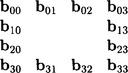
The problem: find the control net of a Bézier surface that fits between the boundary curves.
Figure 7.13illustrates the construction of the Coons patch. In order to find the interior control points bi,j, first construct a point on each of the following ruled surfaces:
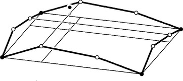
Figure 7.13 Coons patches: the construction. Gray points, from bottom: bu,v1,2,bu1,2,bv1,2. Above them, solid black: b1,2.
Next, construct a point on the bilinear interpolant to the four corner points:
The final control point is created as a combination of these three points:
7.4.2 Tensor Product Interpolation
Tensor product interpolation is suitable for data which has a rectangular structure. More precisely, the given data consist of an (m + 1) × (n + 1) array of data points xij; 0 ≤ i ≤ m, 0 ≤ j ≤ n, and each point has an associated parameter value (ui, vj). A tensor product Bézier patch may be written in matrix form:
Interpolation requires that (7.25) hold for each pair (ui, vj). This results in (n + 1) × (m + 1) equations, which may be written concisely as
where
The matrices U and V already appeared in section 7.2.1; they are Vandermonde matrices. In an interpolation context, the xijare known and the coefficients bijare unknown. Theoretically they may be found by setting
The inverse matrices in (7.27) exist since the functions Bmi and Bnj are linearly independent.
The practical method for finding the control points centers on the tensor product property, as discussed in the chapter 4on Bézier Techniques. Following the schematic diagram in Figure 7.14, the key is to break the problem down into two sets of curve interpolation problems. This is apparent by rewriting (7.26) as
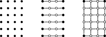
Figure 7.14 Tensor product interpolation: left, the data points; middle, interpolating all rows of data points; right, interpolating all columns from previous step.
where
Equation (7.28) should be rearranged to follow the normal linear system format, that is
Thus, first solve (n+1) univariate degree m interpolation problems in (7.30), one for each row of XT and D, where Dcontains the unknowns. This is illustrated in the middle of the figure by the six cubic interpolants - the “rows.” Next, solve (m+1) univariate degree n interpolation problems in (7.29), which results in B. In the figure, this corresponds to four degree five interpolation problems, schematically represented by the middle and right most diagram. It is important to note that the coefficient matrix is the same for all interpolation problems in the two stages of this algorithm.
7.4.3 Approximation with Tensor Product Patches
Often times the data do not come in a rectangular structure, as expected in the tensor product interpolation of section 7.4.2. This is particularly true with the advent of laser digitizers. Even if the data points have a rectangular structure, it may be nontrivial to find parameter values such that the univariate curve problems produce reasonable solutions. Approximation allows for a more flexible surface construction method.
Suppose the given data consists of a set of points pk, k = 0,…, K. Also assume that each data point pkis associated with a corresponding pair of parameters uk = (uk, vk). Approximate this data by a degree (m, n) Bézier patch. For “best” results, the number of data points should well exceed the number of points needed for interpolation: (K +1) > (m +1) × (n + 1). To aid in the construction of the approximant, the Bézier patch will be written using a linearized notation:
The best approximating surface would result in each data point lying on the approximating surface. For the k—th data point pk, this becomes pk = x(uk) or
Combining all K +1 of these equations results in
which may be abbreviated to
These are K +1 equations in (m + 1)(n + 1) unknowns. If there are many more data points than control points, then the linear system (7.34) is overdetermined. A “good” approximation is found by forming
Notice that this approach mimics that used in section 7.2.2, therefore this is the least squares solution to the approximation problem. A note of caution: if the number of data points is very large (105 or more), then the normal equations become ill-conditioned and the least squares problem may become unstable.
Defining Parameter Values
In a practical setting, one would not typically be given the parameter values uk = (uk, vk). Finding good values for the ukis not always an easy problem. Three solutions are described in this section.
If the data points can be projected into a plane then finding good parameters is not difficult. Assume they can be projected into the (x, y)-plane for simplicity. Each pkis projected by simply dropping its z—coordinate, leaving a pair (xk, yk). Scale the (xk, yk) so that they fit into the desired domain, and then set uk = xk and vk = yk.
If the data can be projected onto a cylinder then finding parameters is also not difficult. For example, assume they can be projected onto the cylinder
When each pkis projected onto the cylinder, the projected point’s (θk, zk) coordinate will correspond to the parameters of pk. Of course an actual projection is not necessary. Here, the value of θ is determined by a calculation in the (x, y)-plane, and zk is directly extracted from pk. Finally, scale all (θk, zk) to live within the desired domain.
For less structured data, it might be necessary to use a more sophisticated method. First, obtain a triangulation of the data points. This scenario is realistic for data obtained using a laser digitizer. Assuming that the triangulation is isomorphic to the unit square, we can construct a triangulation in the unit square with the same connectivity as the given one in 3D. The following method is due to Floater [14]. First, a convex polygon is built in the (u, v) unit square with as many vertices as the 3D mesh has boundary vertices. This polygon is somewhat arbitrary; a circle or the boundary of the unit square are good candidates for forming it. In this way, we assign 2D parameters to the 3D mesh boundary points. Next, consider any interior point uof the 2D mesh with n neighbors. These neighbors are labeled u1, …, un. For a “nice” triangulation, the following condition should be satisfied for each interior u:
We now observe that there are as many equations (7.36) as there are (unknown) interior points in the mesh. Some of these equations involve boundary points, others will not. This system is always solvable.
Shape Equations
One of the points of using Bézier techniques is the benefit of a polygon that closely resembles the shape of the underlying curve or surface. However, the solution to a least squares problem in section 7.4.3 may be close to the data points, yet the control net might “behave badly,” similar to the curve case as illustrated in Figure 7.7. As with curve approximation, a way to combat such behavior is to invoke shape equations. These are conditions that a “good” control net would satisfy. A translational surface, which is characterized by the fact that its twist vanishes everywhere, has a very well-behaved polygon. In terms of the control net, this means that
When these equations are added to the overdetermined linear system (7.34), the result will be less faithful to the data points, but it will achieve a control net with better shape. In practice, one would weigh the shape equations, just as was done for the curve case.
7.4.4 Bicubic Hermite Patches
Many surface schemes are generalizations of curve schemes. Bicubic Hermite patches follow that rule, as they are a generalization of cubic Hermite interpolation from section 7.2.3. Again, to gain more control over the interpolant, derivatives are introduced to the given information. As illustrated in Figure 7.15, the given data for this interpolation problem include points, partials, and mixed partials at each corner:
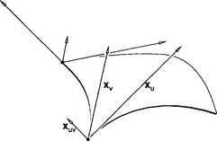
Note how the coefficients in the matrix are grouped into four 2×2 partitions, each holding the data pertaining to one corner. Additionally, the parameter space must be given, for instance, define the patch over u0≤ u ≤ u1and v0≤ v ≤ v1.
Employing knowledge of the Hermite basis functions from section 7.2.3, the interpolating bicubic Hermite patch takes the following form:
Keep in mind that the Hi3 must incorporate the parameter interval, as defined in (7.15).
In order to define the bicubic Bézier representation of this patch,
the control points must be defined. First, the corner points are simple assignments:
The boundary control points are computed using the curve algorithm from section 7.2.3, for example
Recall from the Bézier Techniques chapter 4that the mixed partials at the corners of a Bézier patch take a very simple form, for example at one corner of the bicubic patch,
where Δu = u1- u0and Δv = v1- v0. Therefore, the middle, or twist control points are assigned as follows
Thus the bicubic Bézier patch, which interpolates to Hermite data, has been completely defined.
7.5 C2 BICUBIC SPLINE INTERPOLATION
In an interpolation context, if given point data come in a rectangular structure, often times there will be too many points to realistically use one polynomial patch, as was done in section 7.4.2. Higher degree patches have a tendency to oscillate. An alternative approach is to employ bicubic Hermite patches, however generation of the necessary derivative data is not trivially done in a meaningful manner. The most popular solution to this problem are tensor product bicubic B-spline surfaces. The principles from section 7.4.2 apply here too.
Suppose we are given (K + 1) × (L + 1) data points xI Jand two knot sequences u0, …, uKand v0, …, vL. This interpolation method will employ a bicubic tensor product B-spline surface,
which has triple knots at each end of the two knot sequences and simple knots elsewhere. This special requirement results in the relationships M = K + 2 and N = L + 2, that is, the final B-spline control net has two more rows and columns than the given data point array. The given knot sequences correspond to the unique knots in the knot sequences of the B-spline surface. The solution to this interpolation problem constitutes finding the dij.
Figure 7.16illustrates the steps necessary to define the interpolating B-spline surface. For each row of data points, prescribe two end conditions, such as Bessel tangents, and solve the univariate B-spline interpolation problem as described in section 7.3. Since all interpolation problems use the same knot sequence, each problems has the same tridiagonal coefficient matrix, thus an LU decomposition technique should be applied. The points marked by triangles in Figure 7.16 have thus been constructed. Now take every column of points denoted by triangles, and perform univariate B-spline interpolation on it, again by prescribing end conditions. The resulting control points constitute the desired B-spline control net. An example is shown in Figure 7.17. An alternative approach would be to interpolate first to the columns of data points. This would produce the same result, however the computation count for the two processes are not identical.
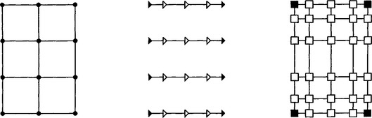
Figure 7.16 Tensor product bicubic spline interpolation: the solution is obtained in a two-step process.
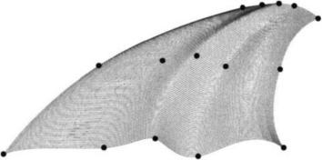
Figure 7.17 Tensor product bicubic spline interpolation: the given data, solid circles, and the solution, using Bessel end conditions and uniform parametrizations.
7.5.1 Finding Knot Sequences
One obstacle to a good interpolant is the generation of one set of parameter values for all isoparametric curves in the u-direction; the same holds for the v-direction. When the data points significantly deviate from a regular grid, the problem of finding an appropriate parametrization can be quite difficult. As discussed in section 7.3.2, a poor choice in parameters can cause an isoparametric curve to unnaturally wiggle, and this defect will be reflected in the surface. One possibility for finding a reasonable parametrization is the following. Create a good parametrization for each isoparametric curve using one of the methods from section 7.3.2. Average each of these parametrizations to yield one. This approach will only produce acceptable results if all our isoparametric curves essentially yield the same parametrization. It is not difficult to find an example for which this will not help. Figure 7.18illustrates from a schematic point of view, the type of distribution of data that will cause this method to fail.
7.6 VOLUME DEFORMATIONS
Once an initial curve or surface is designed, sometimes a deformation of the shape is called for; this would be a bending or stretching of the shape. P. Bézier [1–3] devised an intuitive method to deform a Bézier patch which eliminated the need to tediously move control points. His method also applicable to B–spline surfaces. A more graphics-oriented version of this principle was presented by Sederberg and Parry [28], see also [16].
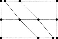
To illustrate the principle, consider the 2D case first. Let x(t) be a planar curve (Bézier, B–spline, rational B–spline, etc.), which is, without loss of generality, located within the (u, v) unit square. Next, cover the square with a regular grid of points
Every point (u, v) may be written as
This follows from the linear precision property of Bernstein polynomials. Now, distort the grid of bi,j into a grid ![]() ; the point (u, v) will be mapped to a point (û,
; the point (u, v) will be mapped to a point (û, ![]() ):
):
which is a mapping of E2 to E2. In particular, the control vertices of the curve x(t) will be mapped to new control vertices, which in turn determine a new curve y(t). Note that yis only an approximation to the image of xunder (7.40).3This is highlighted by the fact that the image of x’s control polygon under (7.40) would be a collection of curve arcs, not another piecewise linear polygon. Figure 7.19gives an example of the use of this global design technique. This technique may be generalized. For instance, we may replace the Bézier distortion (7.40) by an analogous tensor product B-spline distortion. This would reintroduce some form of local control into our design scheme.
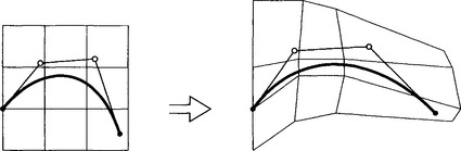
Figure 7.19 Curve deformation: a Bézier polygon is distorted into another polygon, resulting in a deformation of the initial curve.
The next level of generalization is to IE3, and requires the introduction of a trivariate Bézier patch,
which constitutes a deformation of 3D space. Similar to the planar deformation, the control net in (7.41) is used to deform the control net of a surface embedded in the unit cube. Again, the use of a Bézier patch for the distortion is immaterial; trivariate B-splines, for example could have been used too.
A practical example of volume deformations, as illustrated in Figure 7.204, is in brain imaging. In comparative studies, many MRI brain scans have to be compared. Different people have differently shaped brains; in order to carry out a meaningful comparison, they have to be aligned and then they have to be deformed for a closer match - see [30] or [29]. While volume deformations take 3D objects to other 3D objects, it is convenient to visualize the results by a sequence of 2D slices, as shown in Figure 7.20.

1. translated from the French by A.R. Forrest Bézier, P. Numerical Control: Mathematics and Applications. Philadelphia, PA: Wiley; 1972.
2. Bézier, P. General distortion of an ensemble of biparametric patches. Computer-Aided Design. 1978;10(2):116–120.
3. Bézier, P. The Mathematical Basis of the UNISURF CAD System. Butterworths; 1986.
4. Boehm, W., Prautzsch, H. Geometric Foundations of Geometric Design. London: AK Peters; 1992.
5. Burchardt, H., Ayers, J., Frey, W., Sapidis, N. Approximation with aesthetic constraints. In: Sapidis N., ed. Designing Fair Curves and Surfaces. Boston: SIAM; 1994:3–28.
6. Cohen, E., O’Dell, C. A data dependent parametrization for spline approximation. In: Lyche T., Schumaker L., eds. Mathematical Methods in Computer Aided Geometric Design. Philadelphia: Academic Press; 1989:155–166.
7. 1963 Davis, P. Interpolation and Approximation, first edition. Dover; 1975.
8. DeRose, T. Composing Bezier simplices. ACM Transactions on Graphics. 1988;7(3):198–221.
9. Epstein, M. On the influence of parametrization in parametric interpolation. SIAM J Numer. Analysis. 1976;13(2):261–268.
10. Farin, G. Curves and Surfaces for Computer Aided Geometric Design, fifth edition. New York: Morgan-Kaufmann; 2001.
11. Farin, G., Hansford, D. Discrete Coons patches. Computer Aided Geometric Design. 1999;16(7):691–700.
12. Farin, G., Hansford, D. The Essentials of CAGD. AK Peters; 2000.
13. Farouki, R., Rajan, V. On the numerical condition of polynomials in Bernstein form. Computer Aided Geometric Design. 1987;4(3):191–216.
14. Floater, M. Parametrization and smooth approximation of surface triangulations. Computer Aided Geometric Design. 1997;14(3):231–271.
15. Foley, T. Interpolation with interval and point tension controls using cubic weighted v – splines. ACM Trans, on Math. Software. 1987;13(l):68–96.
16. Gomes J., Darsa L., Costa B., Velho L., eds. Warping and Morphing of Graphical Objects. Morgan Kaufmann, 1999.
17. Hartley, P., Judd, C. Parametrization of Bezier-type B-spline curves. Computer-Aided Design. 1978;10(2):130–134.
18. Hartley, P., Judd, C. Parametrization and shape of B-spline curves. Computer-Aided Design. 1980;12(5):235–238.
19. English translation: Fundamentals of Computer Aided Geometric Design, AK Peters, 1993 Hoschek, J., Lasser, D. Grundlagen der Geometrischen Datenverarbeitung. B.G. Teubner; 1989.
20. (6) Lee, E., Choosing nodes in parametric curve interpolation. Presented at the SIAM Applied Geometry meeting. Albany, N.Y., 1987. Computer-Aided Design, 1989;21.
21. Mcconalogue, D. A quasi-intrinsic scheme for passing a smooth curve through a discrete set of points. The Computer J. 1970;13:392–396.
22. Mehlum, E. Nonlinear splines. In: Barnhill R., Riesenfeld R., eds. Computer Aided Geometric Design. Stuttgart: North-Holland; 1974:173–208.
23. Moreton, H., Sequin, C. Minimum variation curves and surfaces for cagd. In: Sapidis N., ed. Designing Fair Curves and Surfaces. SIAM; 1994:123–160.
24. Nielson, G. Coordinate free scattered data interpolation. In: Schumaker L., ed. Topics in Multivariate Approximation. Philadelphia: Academic Press, 1987.
25. Nielson, G., Foley, T. A survey of applications of an affine invariant norm. In: Lyche T., Schumaker L., eds. Mathematical Methods in CAGD. Academic Press; 1989:445–467.
26. Piegl, L., Tiller, W. The NURBS Book, second edition. Springer Verlag; 1997.
27. Runge, C. Ueber empirische Funktionen und die Interpolation zwischen aequidistanten Ordinaten. ZAMM. 1901;46:224–243.
28. (4) Sederberg, T., Parry, S., Free-form deformation of solid geometric models. SIGGRAPH proceedings. Computer Graphics, 1986;20:151–160.
29. Toga A., ed. Brain Warping. Academic Press, 1999.
30. Xie, Z., Farin, G. Hierarchical B-spline deformation with an application to brain imaging. In: Schumaker L., Lyche T., eds. Mathematical Methods in CAGD. Vanderbilt University Press, 2001.
1Note the similarities with the de Casteljau algorithm.
2If the points are on a straight line, but distributed unevenly, the graph of the straight line will be recaptured, but it will not be parametrized linearly.
3An exact procedure is described by T. DeRose [8].
4Courtesy S. Xie and the Arizona Alzheimer Research Center.