Rational Techniques
The following article will focus on rational parametric curves and surfaces and how they are used in geometric modeling applications. Aside from giving an overview of the state-of-the-art, I will emphasize the role of rational techniques in commercial CAD packages.
5.1 INTRODUCTION
Looking at the history of CAGD in industry, it can be argued that rational techniques and representations were at the root of geometric modeling. In particular conic sections and quadric surfaces were the initial building blocks of early CAD systems. Liming [27],[28] detailed many geometric constructions for aircraft design using conics. Later S. Coons at Ford introduced conics into a CAD system; independently conics were used by engineers at Boeing. The quest for compatible formats and for exchanging data among different systems then led to the consideration of standard data formats. The need arose to find a common representation for basic spline curves and conics. Hence the NURBS representation was developed where NURBS stands for Non-Uniform Rational B-Spline. NURBS were first introduced in Versprille’s thesis [43]; later A. Klosterman was instrumental in establishing NURBS as an industry wide standard by choosing them as data representation in SDRC’s modeling software I-DEAS. Today NURBS are integral part of the IGES as well as the STEP standard.
Previous chapters already provided many of the building blocks for developing the material in this chapter. Concepts from projective geometry have been introduced in chapter 2 on Geometric Fundamentals. In chapter 4 on Bézier Techniques, Bézier curves and surfaces have been covered in depth. We will see that many of the algorithms presented there can easily be generalized to the rational case. I will present these algorithms briefly for the sake of completeness; the main focus will be on techniques which are specific to NURBS. Additionally, I will focus on topics related to the practical use of rational representations.
5.2 RATIONAL B éZIER CURVES
In chapter 4 on B ézier Techniques, non-rational B ézier curves have been introduced. In this section, we will generalize these curves to the rational case. Furthermore, we will give a brief outline of standard algorithms and then place special emphasis on algorithms which make use of the additional flexibility offered by rational curves.
5.2.1 Basic definitions
A rational B ézier curve of degree m is a parametric curve which is described by control points, ci ∈ ![]() n, n = 2,3, weights wi and the parameter t. Without loss of generality we let t vary from 0 to 1. The curve has the form
n, n = 2,3, weights wi and the parameter t. Without loss of generality we let t vary from 0 to 1. The curve has the form
The Bernstein B ézier basis functions are defined as
Inspecting Equation (5.1) more closely reveals some simple properties: If we set all the weights wi to 1, then by using the fact that ![]()
![]() (t) = 1, we obtain a non-rational B ézier curve. Furthermore, by ensuring that all wi ≥ 0, and some wi > 0, we can guarantee that the curve does not contain any singularities. The curve c(t) in affine space can be viewed as the projection of a curve
(t) = 1, we obtain a non-rational B ézier curve. Furthermore, by ensuring that all wi ≥ 0, and some wi > 0, we can guarantee that the curve does not contain any singularities. The curve c(t) in affine space can be viewed as the projection of a curve ![]() (t) which lives in projective space and whose control polygon consists of the homogeneous points [wici wi]. Hence, scaling all weights wi by a common factor will not change the underlying control polygon or curve. Rational B ézier curves inherit some properties from the nonrational counterpart:
(t) which lives in projective space and whose control polygon consists of the homogeneous points [wici wi]. Hence, scaling all weights wi by a common factor will not change the underlying control polygon or curve. Rational B ézier curves inherit some properties from the nonrational counterpart:
• Affine Invariance: This is easy to see: We just have to convince ourselves that Equation (5.1) is equivalent to an expression ![]() αiciwith
αiciwith ![]() αi = 1. But this is readily verified by observing that
αi = 1. But this is readily verified by observing that
Here we dropped the parameter t since this reasoning is independent of t.
• Convex hull property: This property holds if wi ≥ 0 ∀i
• Endpoint interpolation: By inserting t = 0 and t = 1 into Equation (5.1), we can verify that
• Variational Diminishing Property: The curve has no more intersections with any plane (or line) than its control polygon has. This can be seen by considering corner cutting algorithms. Corner cutting is equivalent to linear interpolation. Hence each corner cutting step reduces the number of intersections. Using the fact that
degree elevation is an instance of a corner cutting algorithm and repeated degree elevation converges to the curve itself, we have proved the variation diminishing property. Obviously, this property carries over directly from the non-rational case and introducing positive weights does not supply enough additional flexibility to violate this property.
There is one important property of a rational B ézier curve that is not shared by its non-rational counterpart: projective invariance. The curve will stay invariant under general projective transformations. This property can be exploited in graphics algorithms. Instead of applying a projective or perspective transformation to the curve points while rendering (or sampling) the curve, one can first apply the transformation to the control points, and then render the curve subsequently.
Weights and weight points
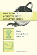
The weights wi can be used as additional shape parameters in the following way. Let us increase a weight wk whereby the other weights are staying unchanged. Then the αk in Equation (5.3) increases as well. This means that the control point ck is weighted more heavily, hence the curve moves closer to the control point ck. This effect is illustrated in Figure 5.1. Furthermore it is illustrated that for a fixed parameter t0 the points c(t0) lie on a straight line for varying weight wk. An elegant proof of this can be found in [16]. In practice, experienced stylists use the weights to fine-tune the shape of curves and surfaces. Some software packages for example support a dial-box interface which can be used to increase and decrease weights with fine granularity.
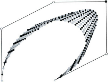
Figure 5.1 The influence of weights on the curve shape. The weight of the black control point is being changed. Note that all the curve points of a fixed parameter lie on a straight line containing the control point with the varying weight.
G. Farin introduced weights points in [13]. These are often called Farin points. The weight points qi are defined as
In Figure 5.2 we illustrate the effect of weight points on the curve. The weights are related to the weight points by the following formula:
This equation shows that if we set w0 = 1 without loss of generality, then the weights are uniquely determined by the weight points. Hence, weight points can be used as shape handles as alternative to using the weights themselves. Farin[15] discovered that rational B ézier curves are not only contained within the convex hull formed by their control points. They are also contained within the convex hull formed by the two end control points and the weight points. Hence we obtain tighter bounds. This is a useful property for many algorithms as we will see later.
5.2.2 Derivatives
The computation of the derivative of a rational B ézier curve can be performed by using the quotient rule. For the first derivative we can perform the following manipulations which are equivalent to rewriting the quotient rule:Define
Then we can compute
Rewriting the derivatives in this way we only need to compute derivatives of polynomial expressions. By using the Leibniz rule, this carries over to higher order derivatives:
This formula is recursive and by using this recurrence relation together with equation (5.6), we can compute any derivative by computing the derivative of non-rational B ézier curves. This can be done efficiently using the de Casteljau algorithm (see chapter 4 on B ézier Techniques). It is easy to see that the derivative of a rational B ézier curve can not simply be obtained by computing the derivative of a non-rational B ézier curve in 4D homogeneous space and subsequent projection. This has implications for piecing together such curves. If two rational B ézier curves have a common derivative in homogeneous space then they will have a common derivative in affine space. The opposite however is not true. We will revisit this topic in the section on geometric continuity. The first order derivatives at the two end points of a rational B ézier curve can be computed quite easily: by using our knowledge from the non-rational case we obtain:
5.2.3 Fundamental algorithms
In the following we will discuss some of the most basic algorithms which are the foundation for evaluating and manipulating rational B ézier curves. We start with the classical algorithm for evaluating rational curves, the de Casteljau algorithm. For rational curves there are two variants of the de Casteljau algorithm. Variant 1 is the straightforward generalization of the non-rational case: The setting here is the projective space and we treat the curve as having homogeneous control points [wici, wi], i = 0,…, m.
de Casteljau Algorithm I: Given: Homogeneous control points ![]() i:= [wici wi], i = 0,…, m and parameter t ∈ [0,1].
i:= [wici wi], i = 0,…, m and parameter t ∈ [0,1].
Find: Point c(t) on the curve in affine space.
Here π is the projection operator. We apply π to the curve ![]() (t) by applying π to every control point.
(t) by applying π to every control point.
The second variant of the de Casteljau algorithm consists of projecting every intermediate point into affine space (see Farin [13]) and is therefore more geometric:
de Casteljau Algorithm II: Given: Homogeneous control points ![]() i:= [wici wi], i = 0,…, m and parameter t ∈ [0,1].Find: Point c(t) on the curve in affine space.Compute
i:= [wici wi], i = 0,…, m and parameter t ∈ [0,1].Find: Point c(t) on the curve in affine space.Compute
Floater [18] points out that the derivative formulae in the previous section do not yield any geometric insight. He rewrites the first derivatives using the intermediate weights and points from the de Casteljau algorithm. One advantage of this formulation is the ease by which one can derive upper bounds for the derivatives of a curve. This is important for many divide and conquer algorithms in practice. For example, when computing curve-curve intersections, one often needs to decide quickly how flat a given segment is.
The next important algorithm is the reparameterization algorithm. It is common to transform rational B ézier curves into a standard representation. This means that the two end weights w0 and wm are both 1. It is known (see [14]) that two rational B ézier curves c and ![]() describe the same shape if their weights are related by
describe the same shape if their weights are related by ![]() , where f is an arbitrary scalar. Since we can scale arbitrarily, it is obvious how to achieve one weight being equal to 1. Let us now assume that w0 = 1. If we set
, where f is an arbitrary scalar. Since we can scale arbitrarily, it is obvious how to achieve one weight being equal to 1. Let us now assume that w0 = 1. If we set
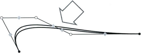
we have achieved that wm = w0. Dividing by w0 yields the curve in standard form. It should be noted that changing the parameterization of the curve in this manner has practical implications. Figure 5.3 shows how the parameter spacing is changed. In practice, one often evaluates curves in equal parameter increments just as in Figure 5.3. This indicates that the parameterization has to be taken into account to avoid sampling artifacts. In [10], a projective parameterization was introduced which allows an evenly spaced sampling of a full circle. On the other hand, this also shows that an injudicious choice of weight factors can substantially skew the parameterization of a curve.
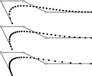
Figure 5.3 Effect of parameterization on sampling density, f = 2 (top), f = 1 (middle), and f = 0.5 (bottom).
Another useful technique is degree elevation. This is the process of raising the degree of a m-degree curve to a larger degree n. This technique is useful in practice for building a surface from cross sections; this process is called lofting. In order for the resulting loft surface to interpolate the sections, all sections have to be of identical degree. One way to achieve this is to perform degree elevation. The degree elevation algorithm for rational curves is a straightforward generalization of the non-rational case. Its setting is the projective space with homogeneous control points.
Degree Elevation: Given: A B ézier curve c(t) of degree m with homogeneous control points ![]() i:= [wi,ci wi]. Find: The B ézier curve d(t) of degree m + 1 such that d ≡ c on [0,1].
i:= [wi,ci wi]. Find: The B ézier curve d(t) of degree m + 1 such that d ≡ c on [0,1].
Here we set c−1 = cm+1 = 0. The interplay between degree elevation and reparameterization has been investigated in [14]. One can first degree elevate a given curve c in standard form to obtain a new curve ![]() . Then one can reparameterize the curve c and subsequently degree-elevate this curve. Bringing the degree-elevated curve into standard form yields a curve
. Then one can reparameterize the curve c and subsequently degree-elevate this curve. Bringing the degree-elevated curve into standard form yields a curve ![]() . The curves
. The curves ![]() and
and ![]() describe the same curve but have different control polygons and weights. This is a distinction from the non-rational case where the degree-elevated representation is unique.
describe the same curve but have different control polygons and weights. This is a distinction from the non-rational case where the degree-elevated representation is unique.
In the polynomial case it is easy to tell if a curve of degree m is actually of degree m − 1. One just needs to check that the m-th derivative is identically 0. This is equivalent to check that the m-th difference of B ézier points is equal to 0. The same approach can be taken for rational curves in projective space.
As mentioned in chapter 4 on B ézier Techniques, one is often interested in the opposite direction as well; that means one would like to find a curve of a lower degree which represents the given curve of higher degree. This problem often occurs in practice, when one needs to exchange data between different CAD systems. Some CAD systems can handle curves and surfaces of higher degrees than other systems. It is easily seen that in most cases there will be no exact solution. Eck [11],[12] and many others gave algorithms for degree reducing non-rational B ézier curves. There are not many algorithms for degree reducing rational curves specifically. Assuming that we have an algorithm for non-rational curves we can try to apply this algorithm to the homogenous coordinates. However it is not guaranteed that the weights remain positive.
5.2.4 Conics
Conic sections can be represented exactly as a rational quadratic B ézier curve. Without loss of generality, we can assume that the two weights w0 and w1 are equal to 1. This means that a conic section c(t) has the representation
with t ∈ [0,1]. For a conic in this representation it is always true that the shoulder point of the conic is at parameter value t = 1/2. Furthermore, the tangent at the shoulder point, often called the shoulder tangent, is parallel to the line connecting b0 and b2. Another interesting fact is that by reversing the sign of w1 we obtain the complementary conic segment ![]() (t). It is easy to show that the three points b1, c(t) and
(t). It is easy to show that the three points b1, c(t) and ![]() (t) are always collinear. It is well known, that in affine space, there are three classes of conics: hyperbolas, parabolas and ellipses. It is now natural to ask if this classification can be performed based on the above representation. Since hyperbolas have two singularities and parabolas only one, it is also intuitively clear that the weight w1 plays a crucial role, because this is the only parameter affecting the denominator. It turns out that indeed we can classify conics by inspecting the weight w1, or more precisely, solve the quadratic equation given by the denominator of the complementary segment:
(t) are always collinear. It is well known, that in affine space, there are three classes of conics: hyperbolas, parabolas and ellipses. It is now natural to ask if this classification can be performed based on the above representation. Since hyperbolas have two singularities and parabolas only one, it is also intuitively clear that the weight w1 plays a crucial role, because this is the only parameter affecting the denominator. It turns out that indeed we can classify conics by inspecting the weight w1, or more precisely, solve the quadratic equation given by the denominator of the complementary segment:
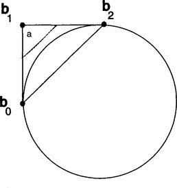
One sees that for w1 > 1 we have two zeros and hence two singularities, yielding a hyperbola. The case w1 < 1 yields an ellipse and for w1 = 1 we obtain a parabola. The latter is obvious, since this means that the curve is a non-rational quadratic, hence it must be a parabola. We will now look at some specific constructions. The first is a circular segment that is a special case of an ellipse. We know that the weight w1 must be greater than 0 and smaller than 1. Due to the symmetry we also know that the control points b0, b1, and b2 must form an isosceles triangle. It turns out that w1 = cos(α) where α is the angle formed by the lines ![]() and
and ![]() (see Figure 5.4). In order to obtain a full circle, one needs to piece together several segments, for example one could piece together 3 segments each with angle α = 60 degrees. Another construction that is often used in practice, in particular for constructing blend surfaces is the so-called ρ-conic (see [30]). Here we prescribe the two endpoints b0 and b2 as well as the end tangents hereby defining the point b1. Additionally, the shoulder point p at t = 1/2 is restricted to lie on the line joining b1 and the midpoint pm of
(see Figure 5.4). In order to obtain a full circle, one needs to piece together several segments, for example one could piece together 3 segments each with angle α = 60 degrees. Another construction that is often used in practice, in particular for constructing blend surfaces is the so-called ρ-conic (see [30]). Here we prescribe the two endpoints b0 and b2 as well as the end tangents hereby defining the point b1. Additionally, the shoulder point p at t = 1/2 is restricted to lie on the line joining b1 and the midpoint pm of ![]() . This means that p − pm = ρ(b1 − pm) where ρ is the parameter sliding the point up and down the line and hence pulling the conic closer or farther away from p1. One could say that ρ describes the “fullness” of the curve. It turns out that the corresponding weight w1 can be computed as
. This means that p − pm = ρ(b1 − pm) where ρ is the parameter sliding the point up and down the line and hence pulling the conic closer or farther away from p1. One could say that ρ describes the “fullness” of the curve. It turns out that the corresponding weight w1 can be computed as
where the τi are the barycentric coordinates of p with respect to the triangle formed by the control points. Note that this equation is always solvable if p lies inside the triangle, but it might not be solvable otherwise. The construction described above is a special case of the classic construction of a conic from two points and their tangents and an additional point. More on conics in B ézier form can be found in [30].
5.3 RATIONAL B-SPLINE CURVES
In chapter 6 on Spline Basics, the basic theory of splines as pioneered by Schoenberg [39] has been developed. Just as is the case for B ézier techniques, we can generalize non-rational B-Splines to the rational case. This defines non-uniform rational B Splines (NURBS) which are the current industry standard. Here we will deal with rational B-Spline curves, so we present the basic definitions first.
5.3.1 Basic definitions
A NURBS curve of degree m is given by: control points also known as de Boor points di, i = 0,…, n, di ∈ ![]() k, k = 2, 3.weights wi, i = 0,…, n,knot vector τ = {t0, …,tn+m+1}.
k, k = 2, 3.weights wi, i = 0,…, n,knot vector τ = {t0, …,tn+m+1}.
We assume that the first and last knots have multiplicity m+1 each. This is industry-wide convention and it ensures end point interpolation.
A rational NURBS curve d(t) is defined as
The normalized B-Spline basis functions are defined recursively:
where
The properties of these basis functions are discussed in detail in chapter 6 on Spline Basics. We can now proceed as in the B ézier case and define the curve as a linear combination of control points:
with
This leads immediately to the following properties:
The degree elevation and knot insertion algorithms can again be viewed as examples of corner-cutting algorithms and this can be used to prove the variation diminishing property just as in the B ézier case. Furthermore, we can easily deduce that the NURBS curve as defined above interpolates the endpoints:
The effect of the weights on the curve is similar to B ézier curves. Increasing the weight wi relative to its neighbors causes the curve to move towards the control point di.
5.3.2 Derivatives
In order to compute derivatives of rational B-spline curves, we proceed in the same manner as for rational B ézier curves. We define
where w(t) is the 1D B-Spline weight function, and again arrive at the equation
Now we just need to recall how to compute derivatives of a non-rational B-Spline curve p(t).
Higher order derivatives can be computed by using the recurrence relation for the B-Spline basis functions. A different approach for computing the first derivative of a NURBS curve has been developed by Floater [19]. Assuming that the parameter t is contained in [tI,tI+1], and using
one can show that the NURBS curve d(t) obeys:
with
Floater uses this expression to derive upper bounds for the derivatives.
5.3.3 Fundamental algorithms
In chapter 6 on Spline Basics different algorithms for evaluating B-Spline curves have been presented. One can directly make use of the recurrence relation. Alternatively one can use knot insertion or the Oslo algorithm to evaluate a spline. The most commonly used algorithm is the de Boor algorithm. This algorithm can be viewed as a generalization of the de Casteljau algorithm. Again we can give two versions, the first version using homogeneous coordinates:
de Boor Algorithm I: Given: Homogeneous control points ![]() := [widi wi], i = 0,…, n, knot vector τ = {t0,…, tm+n+1} and parameter t. Find: Point d(t) on curve in affine space.Compute I such that t ∈ [tI, tI+1) ⊂ [tm, tn+1].
:= [widi wi], i = 0,…, n, knot vector τ = {t0,…, tm+n+1} and parameter t. Find: Point d(t) on curve in affine space.Compute I such that t ∈ [tI, tI+1) ⊂ [tm, tn+1].
with ![]() .
.
Here we used the convention that r denotes the multiplicity of t in case t is an element of the knot vector, and 0 if t is not contained in the knot vector. In analogy to the B ézier case we can define a rational version of the de Boor algorithm:
de Boor Algorithm II: Given: Homogeneous control points ![]() i:= [widi wi], i = 0,…, n, knot vector τ = {t0, …,tm+n+1} and parameter t. Find: Point d(t) on curve in affine space.Compute: I such that t ∈ [tI, tI+1) ⊂ [tm,tn+1].
i:= [widi wi], i = 0,…, n, knot vector τ = {t0, …,tm+n+1} and parameter t. Find: Point d(t) on curve in affine space.Compute: I such that t ∈ [tI, tI+1) ⊂ [tm,tn+1].
with k = 1,…,n -r and i = I - n + k + 1,…, I - r + 1. As pointed out before, this version uses convex combinations and hence is more stable. On the other hand the operations count is increased.
Reparameterizations
It is possible to reparameterize a NURBS curve. The key observation is due to Lee and Lucian [31]: If we apply a rational linear (Moebius) parameter transformation to a NURBS curve, the resulting curve is again a NURBS curve with the same control polygon but different weights and knots. More precisely: Define the linear rational map φ by
If we apply this transformation to a NURBS curve with knot vector τ we obtain a curve with knot vector ζ = {s0, …, sn} and si = φ(ti). The new weights are given by
Since the rational linear map has 3 variables (set α = 1 without loss of generality), we can now pick the unknowns in such a way that ![]() and
and ![]() are equal. This leads to a NURBS curve in standard form (see [31]). Conversely, one could also try to determine the unknowns in such a way that intermediate knots are mapped to certain target values. However, this seems to be of limited use since in most cases one would have to solve a least squares system and the new weights are unbounded.
are equal. This leads to a NURBS curve in standard form (see [31]). Conversely, one could also try to determine the unknowns in such a way that intermediate knots are mapped to certain target values. However, this seems to be of limited use since in most cases one would have to solve a least squares system and the new weights are unbounded.
5.4 GEOMETRIC CONTINUITY FOR RATIONAL CURVES
In this section we will address the topic of geometric continuity for rational curves. If we recall how we derived the derivatives of a rational B ézier curve, it is easily seen that C1 continuity in projective space implies C1 continuity in affine space but the reverse is not true. We abbreviate continuity in projective space with HCk or HGk respectively, whereas continuity in affine space is denoted by Ck or Gk. Let us start with two B ézier curves of degree m where the first curve has a control polygon c0,…, cm, weights w0,…, wm and is defined over the interval [u0, u1]. The second curve has control points cm,…, c2m and weights wm,…, w2m and is defined over the interval [u1, u2]. Furthermore, we define δ0:= u1 - u0 and δ1:= u2 - u1. If we recall the results in section 5.2.2, it turns out that the two curves are C1 continuous at u1 if
One can also see that for G1 continuity the weights do not play any role at all. In [5] conditions for curvature and torsion continuity of rational B ézier curves have been derived. These conditions have nice geometric interpretations: Let us define the following quantities:
Here T+ is the tangent defined by cm and cm+1, T- is the corresponding tangent defined by cm and cm−1. Furthermore, O+ is the osculating plane spanned by cm, cm+1, and cm+2, whereas O- is the osculating plane spanned by cm, cm-1, and cm−2. The two curves are curvature continuous or G2 continuous if they are C1 continuous, the 5 points cm−2,…, cm+2 are coplanar, cm−2 and cm+2 lie on the same side of tangent T+ (which is equal to T_ in that case) and the following relationship holds:
For a non-planar rational B ézier curve, the conditions for torsion continuity are also of practical interest. Two curvature continuous rational B ézier curves are torsion continuous at cm if cm−3 and cm+3 lie in different half spaces defined by the osculating plane O+ (by assumption O+ equals O-), and the distances obey
In Figure 5.5 we illustrate the geometry and the quantities involved for defining curvature and torsion continuity, including the G1 condition. In [5], Boehm also presents construction algorithms for curvature continuous cubic B-Splines as well as torsion continuous quartic B-Splines. The algorithms make use of the interplay of B ézier control points and de Boor points. The de Boor points di can be derived from the intersection of segments formed by the B ézier control points.
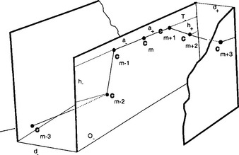
Figure 5.5 Construction of curvature and torsion continuous curves. We depict all the control points and scalar quantities (distances) that are involved.
One should note that the above conditions and constructions are valid in affine space but they do not guarantee homogeneous continuity. For this to achieve one has to investigate continuity in projective space using homogeneous coordinates. Degen [7] derived conditions for Gr continuity using homogeneous coordinates. He showed that for two curves to be Gr continuous, there needs to exist a triangular matrix which transforms the control points from the first curve directly into the control points for the second curve. Furthermore, he gives a recurrence formula for Gr conditions with arbitrary r.
5.5 RATIONAL CURVE APPROXIMATION AND INTERPOLATION
In practical applications, one of the most common and important tasks is to approximate or interpolate point data. Furthermore, one often needs to approximate curves which are given in analytical form but are not representable exactly as NURB curve. Examples of these are intersection curves or offset curves. It is also a fact that in most commercial software packages, the weights are not used when approximating or interpolating with NURB curves, it would be more accurate to talk about NUB curves. It remains the case that the main justification for using true rational curves in practice is their ability to represent conics and circles exactly. Their use is mainly limited for that purpose. The reason why the weights are not utilized for fitting is twofold:
•1) Treating weights and control points as unknowns immediately requires the solution of a nonlinear problem.
•2) The desired range of values that weights should attain is rather restrictive. Weights should be positive, be bounded away from zero and also have a reasonable upper bound when we assume standard form. More precisely, one often prescribes weights to be in the range f * [0.5,2.0] where f is a common factor.
Nonetheless, algorithms have been developed to use the weights for fitting. We will present the relevant work below.
5.5.1 Rational curve interpolation
The direct approach to rational curve interpolation is to consider data points in projective space and then interpolate in homogeneous coordinates just as can be done in the nonrational case: Given are data points pi and weights vi and corresponding parameters ti, i = 0,…, n. In 4D we compute a rational spline curve c(t) such that c(ti)T = [vipi vi]. This problem can be solved analogously to the non-rational case. The heuristics for choosing knots can also be taken from the nonrational case. The problem is however somewhat ill-posed, since in practice we usually have only data points but not the weights. There is no algorithm for choosing weights; in addition, solving this problem globally can easily produce weight functions with singularities. A different and more practical approach has been investigated by Schneider in his Ph.D. thesis [37]. Here, the weights are treated as additional unknowns; this allows to specify more data points. Concretely, it turns out that if we have m + 1 data points, a curve with n + 1 de Boor points can be determined uniquely if the relation n = 3m/4 holds. The interpolation problem is then solved using homogeneous coordinates. One of the remaining problems is that the resulting interpolation curves can exhibit singularities. Even more interestingly, the parameterization has an effect on this, there are cases where by using chord length parameterization the curve exhibits singularities whereas by using centripetal parameterization the curve has no singularities, however it interpolates the same data. A practical concern is that many times curves are constructed as building blocks for surfaces. This poses severe limitations on the parameterization. As evidenced above, the rational interpolation problem is very sensitive to the parameterization, even more so than in the non-rational case.
For reasons outlined above the more practical interpolation methods are those which are based on osculatory interpolation. The basic idea here is that one pieces together locally fitted pieces with prescribed continuity. For example, let us assume we have data points pi, tangents qi, and curvature values κi, or alternatively curvature vectors Ki, i = 0,…, n. We parameterize the data yielding parameters ti. We can now fit say rational cubic B ézier curve segments ci such that ci(0) = pi, ci(1) = pi+1 and furthermore the unit tangent of ci at 0 and 1 equals qi and qi+1 respectively. In addition, the curvature of ci at 0 equals κi and at 1 it equals κi+1. Hoellig proved in [23] that such a curve exists under certain restrictions on the geometry induced by the data. Furthermore, he gave a method to compute such a rational spline curve. Note that this construction is closely related to the continuity conditions we derived earlier. It turns out that this method has approximation order 6 which is an improvement over non-rational methods which can only achieve order 4 in the general case. Another popular approach to osculatory interpolation is to use piecewise conic segments. This method is constrained to planar data and makes use of the fact that 5 data points determine a conic uniquely. One approach is to fit conics locally to five data points each and piece the segments together. In general the resulting spline will only be C0 continuous. A more useful approach is to prescribe three data points p0, p1, p2 and two end tangents q0 and q1. If the middle point p1 is contained within the triangle formed by p0, p2 and the intersection of the two tangents q0 and q1, then there is a solution. The resulting interpolating spline is convexity preserving and G1 continuous. Schaback [36] gives a method to construct these segments. It is also possible to prescribe curvature values κ0 and κ1 at the endpoints of a segment together with three data points. In general these constraints can not be satisfied, in [36] Schaback gives conditions that ensure the existence of a unique interpolant. It turns out that these conditions are satisfied if one samples dense enough a smooth regular curve with non-vanishing curvature. Goodman et al. [22] presented a method for fitting planar data with piecewise cubic rational B ézier segments. Their goal was to compute shape-preserving interpolants: if all data points lie on one side of a given line, then the interpolant should not cross that line. Their method proceeds by first computing a G2 continuous rational cubic spline matching two positional and two curvature constraints at the ends. If one of the spline segments violates the line condition, the two interior weights are modified until the curve just touches the line. Obviously this will cause a G2 discontinuity with the neighboring segment and so the weight of the neighboring segment needs to be modified as well.
Note that the osculating interpolation methods can also be viewed as approximation methods, in the case that the data is sampled off a given curve that needs to be fitted by NURBS.
5.5.2 Rational curve approximation
The classical scheme for performing approximation with rational curves is the Padé scheme. Let us briefly go back to the functional setting. We assume that we have a function F(x) that has a Taylor expansion
We are interested in a rational polynomial function R(x) that approximates F. R is of the form
By matching degrees of freedom we can easily see that we have m + n + 1 free coefficients (b0 can be normalized to 1) and hence the best approximation order one can hope for is O(n + m + 1). One computes the approximant by multiplying both sides by the denominator of R and obtains a system of equations that can be solved uniquely if the Hankel determinant of the denominator of R is nonzero. This gives rise to many interesting theoretical investigations. An introduction can be found in [6], other references are [1],[21]. For CAGD applications, it is more useful to use multi-point approximation schemes, in particular the two-points schemes that have been introduced in the previous section. We can construct a parametric Padé approximant that approximates a given function up to a certain order at two parameter values [45]. Here is the problem statement for approximating a curve at two points up to order 2:Given: A parametric curve F(t) = (x(t),y(t), z(t)).Find: A rational B ézier curve b(t) such that
where t ∈ [t0, t1]. There are several strategies for solving this problem. For example one could solve two one-point problems and blend the results, or one could solve three one-dimensional two-point problems and subsequently multiply to make the denominators equal. In [45] a two-points problem was solved for all three components simultaneously. This allows to use a rational polynomial of degree 4 over 4. This is of lower degree than was possible before ([3]). Results show that this approximation method is very effective and that high quality C2 approximations can be obtained.
A variety of different approximation schemes can be found in the literature. The most general scheme treats control points, weights and nodes as free and solves a non-linear optimization problem. Obviously, it will be challenging to avoid getting stuck in a local minimum. Other more specialized methods can be found for example in [2],[44]. In [46],[8] some geometrically motivated methods are presented to approximate smooth curves by rational B ézier curves. Finally, a somewhat different application is the fairing of curves. Here, one is interested in smoothing a curve, most often one would like a smooth change in curvature without spikes. In [24], a method is developed that automatically adjusts the weights of a B-Spline curve. The goal is to produce a curve with smoother curvature variation that is still very close in position to the original curve. Another approach for selecting weights is given in [34].
5.6 RATIONAL B éZIER SURFACES
In this section we will introduce rational B ézier patches. In practice, one of the most challenging problems is the composition of multiple patches. In most cases, one wants to maintain at least G1 continuity to avoid creases. It turns out that this is particularly difficult for rational patches. Hence we will devote a special section to this subject. Furthermore, we will see, that many algorithms for surfaces can be reduced to applying the curve algorithms just as is commonly done for non-rational B ézier patches. However this is not easily possible for approximation algorithms.
5.6.1 Basic definitions
I will briefly introduce rational B ézier patches along with their most important properties; assuming the reader to be familiar with rational curves. A rational B ézier surface of degree m, n is given by an array of control points cij, i = 0,…, m, j = 0,…, n ∈ ![]() 3, and an array of corresponding weights wij. Furthermore we assume a parameterization in s and t where without loss of generality s and t vary from 0 to 1. The patch is defined as:
3, and an array of corresponding weights wij. Furthermore we assume a parameterization in s and t where without loss of generality s and t vary from 0 to 1. The patch is defined as:
We can omit the parentheses in Equation (5.52), I included them for clarity. In the nonrational case, the patch basis functions obey the tensor product condition:
In the rational case the basis functions are
Due to the sum in the denominator a factorization is not possible. This has practical consequences: In order to exploit the tensor product structure, we have to apply the algorithms in projective space using 4 dimensional homogeneous coordinates. Afterwards we have to apply the projection operator π to return into affine space. But one needs to be careful since this approach is not always valid: Remember that for instance derivatives are not correctly computed using this method. We can generalize some of the properties for non-rational patches directly to the rational case:
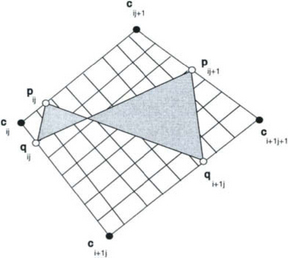
Weights and weight points: By a similar reasoning to the curve case, we can deduce that increasing the value of weight wij relative to its neighbors causes the surface to move towards control point cij. Hence, we can use the weights again as shape parameters. It is also possible to define weight points. We define these points in the s and in the t direction:
Considering the fact, that the weights in s direction and in t direction overlap, it is clear that the pij and qij are not independent of each other. In fact, the relationship is rather constrained: The 4 points pij, pij+1, qij and qi+1j have to be coplanar, see Figure 5.6. Hence it is somewhat more awkward to provide an interface where it is possible to modify surface shape by specifying weight points. A solution to this problem has been proposed by Theisel [42]. There, extended Farin points are first defined in the surface domain and then mapped into 3D. In addition, the author presents a scheme which allows only a subset of the Farin points to be moved in order to avoid conflicting definitions.
5.6.2 Derivatives
Computing partial derivatives of rational B ézier patches is somewhat more complex. I will first give the straightforward derivation and subsequently, I will describe an algorithm by Sederberg that sacrifices the numerical stability of the B ézier basis for a more efficient evaluation of the derivative. For the straightforward version we will proceed very similar to the curve case. Define
Then we have for the two partial derivatives
For higher order partial derivatives, we can again apply Leibniz′ rule and obtain a formula analogous to (5.8). We can also use the approach above to compute mixed derivatives. The general formula is
This expression can easily be transformed to yield the desired mixed derivative of p(s, t). The two first order partial derivatives need to be evaluated repeatedly for rendering a B ézier patch. More precisely, we need the normal vector of the patch and hence we only need the tangent directions but not the derivative magnitude. Sederberg [40] has presented a very efficient method for doing so. As a first step, he transforms the B ézier basis into the power basis to be able to apply the Horner-like scheme which also appears in [17]:
with u = s/(1 − s) and v = t/(1 − t). For stability reasons, one should change the parameter transformation to u = (1 − s)/s and v = (1 − t)/t when either s or t are close to 1. The new control points ![]() ij are computed as
ij are computed as
Incidentally, the formulae (5.63) and (5.64) can be used to evaluate a rational B ézier patch, if we perform the Horner scheme in projective space and perform a subsequent projection. More interesting is the potential for the two tangents: Let us assume for now that the cij are 4D points (homogeneous coordinates). Let us define subpatches:
with
Here α and β vary from 0 to 1. Sederberg then shows that these 4 subpatches combined yield the tangents:
It is further shown that for a surface of degree (n, n) the evaluation algorithm is of order O(n2). This is a substantial improvement over the straightforward evaluation.
5.6.3 Algorithms
In this section some of the most common algorithms will be presented. Let us first present the de Casteljau algorithm for evaluating rational B ézier patches. I will assume that we are performing the computations in projective space, hence we have control points ![]() ij = [wijcij wij]. If we write the patch with the parenthesis as in (5.52) we can readily see the evaluation strategy:
ij = [wijcij wij]. If we write the patch with the parenthesis as in (5.52) we can readily see the evaluation strategy:
If we assume that we want to evaluate the patch at parameter (s0, t0), then the algorithm in pseudo code is as follows:
Compute point Cj(s0) by performing the de Casteljau algorithm for
curve defined by j-th row of control points
Define new curve C(t) of degree n with control points Cj(s0)
Perform de Casteljau algorithm once to evaluate C(t) at parameter t0.
It should be immediately obvious that we could have reversed the roles of i and j and obtain the same result. However, from a practical point of view there is a difference: If the degree in s direction differs from the degree in t direction, a quick operations count shows that it is cheaper to perform more de Casteljau algorithms for a lower degree. So it is advantageous to perform the final de Casteljau algorithm in the direction corresponding to the higher degree. We did not present the direct de Casteljau algorithm for patches. Its non-rational version can be found in [17]. Since it is more complex and also requires case distinctions, it is rarely used in practice.
Reparameterizations
We have seen that rational B ézier curves can be reparameterized such that the end points have weights equal to 1. Obviously, we can perform this reparameterization for either the two s = const boundary curves or the two t = const boundary curves independently. The result will be a patch where the four corner points have weights equal to 1. We can consider such a patch to be in standard form. If we extract a isoparameteric curve from a patch, say the curve corresponding to the i th row of the patch, then the resulting rational curve will not be in standard form. However, we can simply apply the curve reparameterization algorithm to convert this curve to standard form.
5.7 RATIONAL B-SPLINE SURFACES
This section introduces the most important entity in industrial applications, the rational B-Spline surface or NURBS surface. This representation comprises all the surface representations encountered previously: rational and non-rational B ézier patches as well as non-rational B-Spline patches. For surfaces the same is true as for curves: true rational patches are mostly used for representing entities such as cylinders, cones, spheres, tori and surfaces of revolution exactly. However, they are only used to a very limited extent for actual modeling purposes. An exception might be styling application where the weights are used as fairing or sculpting parameters.
5.7.1 Basic definitions
A rational B-spline surface of degree m in s and n in t is given by control points dij, i = 0,…, k, j = 0,…, l, di ∈ ![]() 3.weights wij,i = 0,…, k, j = 0,…,l.knot vectors ζ = {s0,…,sk+m+1}, and τ = {t0,…,tl+n+1}.
3.weights wij,i = 0,…, k, j = 0,…,l.knot vectors ζ = {s0,…,sk+m+1}, and τ = {t0,…,tl+n+1}.
Again we assume that the two knots vectors have start and end knots of multiplicity m + 1 and n + 1 respectively. The NURBS patch p(s, t) is defined as
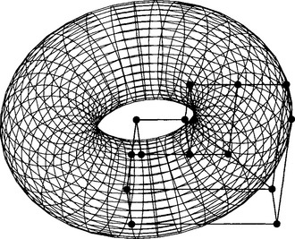
In Figure 5.7 we show a rational B-spline patch. The normalized B-Spline basis functions are the same as encountered before. They allows us to derive some of the properties of NURBS patches:
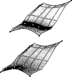
Figure 5.7 Example of a rational B-Spline patch: The top patch below has modified weights such that the vertical fold is more pronounced.
As can be expected, increasing the value of weight wij causes the surface to move towards control point dij.
5.7.2 Derivatives
Computing derivatives follows the same recursive formula as for rational B ézier patches (see (5.62)). Using that formula, the computation of derivatives can be reduced to the computation of derivatives of non-rational B-Spline surfaces. For a non-rational patch q, the following formula holds:
The intermediate B-Spline points ![]() can be obtained as by-products of the de Boor algorithm; their recursive definition is
can be obtained as by-products of the de Boor algorithm; their recursive definition is
From a practical point of view, it might be advantageous to convert the rational B-Spline representation into a rational B ézier representation via knot insertion and then compute the derivatives of rational B ézier patches. This is true for applications that require the evaluation of a large number of points on the patch. The overhead of knot insertion would then be amortized by being able to use Sederberg’s method that has been presented in section 5.6.2. Let us take a special look at the partials at the start and end points of the curve. If we assume multiplicity equal to the order of the surface at the ends, the first partial derivatives can be computed as follows:
5.7.3 Algorithms
The most fundamental task is the evaluation of rational B-Spline patches. There are several options:
• Convert the patch to a rational B ézier patch via knot insertion and apply ‘B ézier’ algorithms
• Use the recurrence relation of the B-Spline basis functions to evaluate the patch in 4D making use of the tensor-product structure
For completeness, we briefly sketch the evaluation procedure using the de Boor algorithm. Assume that we are given a NURBS patch in homogeneous coordinates ![]() (s, t) with a (k + 1) × (l + 1) array of control points
(s, t) with a (k + 1) × (l + 1) array of control points ![]() . Then we can repeatedly apply the de Boor algorithm in the following fashion:
. Then we can repeatedly apply the de Boor algorithm in the following fashion:
Compute point Cj(s0) by performing the de Boor algorithm for curve
defined by j-th row of control points
Define new curve C(t) of degree n with control points Cj(s0)
Perform de Casteljau algorithm once to evaluate C(t) at parameter t0.
We can apply the Moebius transform to each knot vector ζ and τ independently to change the knot spacings. However, it is in general not possible to use the Moebius transformation for manipulating weights. For example, we can not reparameterize a patch in such a way that all the four corner points have a weight equal to 1 since this would require to apply two transformation in say s and hence we would produce two different knot vectors. Hence, this situation differs from the rational B ézier setting.
5.8 GEOMETRIC CONTINUITY FOR RATIONAL PATCHES
As I have mentioned before, when dealing with geometric continuity, it is important to distinguish between continuity conditions in homogeneous setting and affine setting. Affine C1 continuity for example only means that q′ - w′p (with q = wp) is continuous; it does not imply continuity of q′ and w′. The effect is that both quantities independently may have cusps. This can have ramifications for surface construction algorithms. For example isoparametric lines can exhibit cusps that may cause geometry processing algorithms applied to this patch to fail. An example of this can be found in [20]. The remedy for this situation is to construct HG1 continuous patch complexes.
Necessary and sufficient conditions for tangent plane continuity of rational B ézier patches have been developed by Liu [29] and deRose [9]. These conditions treat the rational B ézier patches as polynomial patches in 4-space: Given two patches ![]() (u, u) and
(u, u) and ![]() (u, v) with a common boundary along v = 0, then the patches are G1 continuous if and only if for all points along the common boundary
(u, v) with a common boundary along v = 0, then the patches are G1 continuous if and only if for all points along the common boundary
The situation is illustrated in Figure 5.8.
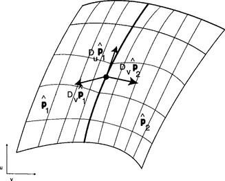
Figure 5.8 Two patches meeting at a common boundary. The depicted derivatives need to be linearly dependent.
Note that this determinant is considered a 4 × 4 determinant in 4 space. In [9] some construction algorithms using this condition are given. This condition is often generalized to the following equation:
where α1(u),β1(u) and γ1 are rational scalar-valued polynomials in u. Analogously, one can derive the conditions for curvature continuity: Two patches p1 and p2 are curvature continuous along a common boundary v = 0 if and only if Equation (5.76) holds and in addition
Again the coefficients α1,2, β1,2 and γ1,2 are rational polynomials in u. They are often called the connection functions. In [47] these conditions are refined and rational expressions for these connection functions are computed. The tangent plane and curvature continuity conditions are the most important conditions in practice. In some cases, it might be necessary to require higher order continuity, for example continuity of the rate of change of curvature (G3). Zheng et al. [48] present some general Gn conditions building upon the framework presented above. The interested reader is referred to this paper. A more in depth treatment of geometric continuity can be found in chapter 8 on Geometric Continuity.
5.9 INTERPOLATION AND APPROXIMATION ALGORITHMS
The interpolation problem for rational patches is often posed as the task of finding a rational patch that interpolates data points pi given in homogeneous coordinates pi = [wx wy wz w]Ti. As pointed out before, there is no good method to determine the weights a priori. An alternative has been proposed by Ma and Kruth [33]. They assume that the parameters for the data points as well as the knot values are given. Then they use the interpolation conditions to set up a system of equations containing the weights and the control points as unknowns. This system is usually overdetermined. The system is transformed so that a two step method can be applied. First one solves for the weights using a singular value decomposition, then one solves for the control points. As an alternative, the weights can be computed by using a constrained minimization scheme in order to keep the weights from becoming negative or otherwise ill-behaved. A very similar method results when applying the method by Schneider [37] presented in section 5.5.2 to surfaces. One just needs to order the array of data points and enumerate them as a list of points. If we have m data points we again need to make sure to have n control points with n = 3m/4.
Even though these methods are feasible in practice, it is more common to look at the problem of approximating a discrete set of points or of approximating a surface given by a different representation. The second problem arises very frequently since NURBS are not closed under operations such as offsetting or surface-surface intersections. Schneider and Juettler [38] presented an approximation technique for curves that can be readily generalized to surfaces: We consider an (k+1) × (l + 1) array of data points qij, i = 0,…, k, j = 0,… l. Assume that we have a rational patch p(s, t) with knot vectors ζ and τ and control points dij and weights wij (i = 0 …, m j = 0,…, n). We want to compute the rational NURBS surface that minimizes
Here W denotes the collection of weights, D denotes the set of control points, and S and T denotes the set of parameters. Note that we leave the parameters free and iteratively adjust these to find a better solution. The adjustment can be performed by using Hoschek’s parameter correction scheme [25]. We can now collect and enumerate all data points and control points in the obvious way: I = is + it * k, is = 0,…,k, it = 0,…, l and J = js + jt * n, js = 0 …, m, jt = 0,…, n. With M = k * l − 1 and N = m * n − 1 we can transform the minimization problem into:
The matrix φ is crucial. It has entries
Note the interplay of two-dimensional indices is,it with I, js, jt with J and hs and ht with H. ks and kt is the degree of the patch in s and t. If we fix an initial parameterization S0 and T0 as well as an initial set of weights W0, we can now compute the control points by applying the pseudo inverse Φ+ of Φ:
To compute or update a set of weights, we need to solve another nonlinear minimization problem:
In order to have a sensible range of the weights, the authors apply a transformation to the wk: ![]() = ∈ + π/2 + arctan(wk) where ∈ > 0 is chosen arbitrarily. The entire method is an iterative process; a) start with an initial parameterization, b) compute a set of weights by performing a non-linear minimization, c) solve for the de Boor points using the pseudo-inverse, and d) perform parameter correction to update the set of parameters. This loop is performed until a desired error tolerance is reached. The reader should note that no proof for the convergence of this method has been given here.
= ∈ + π/2 + arctan(wk) where ∈ > 0 is chosen arbitrarily. The entire method is an iterative process; a) start with an initial parameterization, b) compute a set of weights by performing a non-linear minimization, c) solve for the de Boor points using the pseudo-inverse, and d) perform parameter correction to update the set of parameters. This loop is performed until a desired error tolerance is reached. The reader should note that no proof for the convergence of this method has been given here.
I presented this method here, since this constitutes one of the very few if not the only practical algorithm for using the weights as unknowns to solve the surface approximation problem. Another approach is the method presented in [26]. Here the parameters, the weights as well as the control points are all treated as free variables for the solution of a global minimization problem. Solving this system without getting stuck in the first local minimum requires some preconditioning. Timings show that this method is very inefficient and no geometric insight is applied.
5.10 RATIONAL SURFACE CONSTRUCTIONS
In this section I will briefly cover some of the more important surface constructions involving rational patches.
5.10.1 Surfaces of revolution
A surface of revolution is typically given as
Closer inspection reveals that each isoparametric line v = const traces out a circle with radius r(v). Under the assumption that the generatrix g(v) = [r(v), 0, z(v)]T can be represented in rational form, we can construct the surface using rational B ézier patches. For each vertex of the generatrix, we generate four circular segments in B ézier form (see Figure 5.9).
This yields all the control points. For all midpoints of the circular segments the weights of the generatrix are copied. The other points are assigned these weights multiplied by ![]() . Example of surfaces generated this way are cylinders, tori and spheres.
. Example of surfaces generated this way are cylinders, tori and spheres.
5.10.2 Canal and pipe surfaces
In practice it is often necessary to construct surfaces s(u, v) from a given curve c(v) whose isoparametric curve v = const is a circle with center C(v0) and radius r lying in the normal plane to c(v0). Such surfaces are called pipe surfaces and they can be viewed as generalizations to offset curves in the plane. They can be expressed as
Here n(u, v) is the unit circle with center c(t) lying in the normal plane.
If we assume that the spine curve is rational, then it is clear that we need to find a function n(u, v) with norm equal to 1 and additional constraint that < n(u, v), c′(v) >= 0. In [32] the authors prove the following: if c(v) = [(x(v),y(v), z(v)]T is a rational curve with z′(v) ≠ 0, then the pipe surface with spine c(v) can be rationally parameterized if and only if we can find two rational functions f(v) g(v) such that
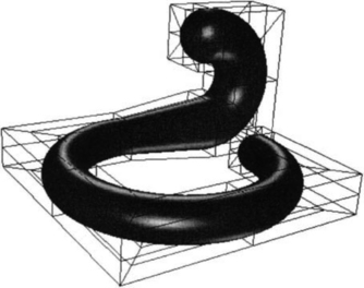
The authors go on to prove that any pipe surface with rational spine curve is rational and give a construction. Furthermore, it turns out that the result is valid for the more general case where the radius r varies with parameter v. Such surfaces are often called canal surfaces. Figure 5.10 depicts a canal surfaces that has been built as a collection of piecewise quadratic rational patches.
5.11 CONCLUDING REMARKS
This chapter gave an overview of rational techniques with particular emphasis on practical applications. Due to space limitations some topics had to be omitted entirely, I also had to made choices on how to present the material. A very important class of surfaces are quadric surfaces. These surfaces can be represented precisely by triangular rational B ézier patches. The reader should consult chapter 31 on Quadrics. In that chapter, the author covers in depth the parametric representation of quadric surfaces using rational B ézier patches. Note that I did not discuss triangular rational B ézier patches in this chapter. Even though they are interesting in their own right, they are not frequently used in practice except for representing quadrics. Unfortunately, the vast majority of commercial CAD packages do not support triangular patches. The interested reader can consult [16],[4].
I chose not to follow the blossoming notation - the reader can get a first glimpse in [17] if so inclined. The theory of blossoms is developed completely in [35]. Furthermore, I did not cover any of the data representation standards in depth. In [16], the reader can find the basic IGES format for NURBS curves and surfaces. NURBS are also included in the STEP standard. The National Institute of Standards is involved in defining STEP; more information can be found in [41].
1. Baker, G.A. Essentials of Padé approximants. Addison-Wesley; 1975.
2. Baumgarten, C., Farin, G. Approximation of logarithmic spirals. Computer Aided Geometric Design. 14(6), 1996.
3. Bajaj, C., Xu, G. NURBS approximation of surface surface intersection curves. Advances in Computational Mathematics. 1994;2(1):1–21.
4. Boehm, W., Hansford, D. Bézier patches on quadrics. In: Farin G., ed. NURBS for Curve and Surface Design. Reading: SIAM, 1991.
5. Boehm, W. Rational geometric splines. Computer Aided Geometric Design. 4(1–2), 1987.
6. Brezinski, C. An introduction to Padé approximations. In: Laurent, Le Méhauté, Schumaker, eds. Curves and Surfaces for Geometric Design. A.K. Peters, 1994.
7. Degen, W. Some remarks on Bézier curves. Computer Aided Geometric Design. 5(3), 1988.
8. Degen, W. High accuracy rational approximation of parametric curves. Computer Aided Geometric Design. 10(3–4), 1993.
9. de Rose, A. Necessary and sufficient conditions for tangent plane continuity of Bézier surfaces. Computer Aided Geometric Design. 7(1–4), 1990.
10. de Rose, A. Rational Bézier curves and surfaces on projective domains. In: Farin G., ed. NURBS for Curve and Surface Design. Boston: SIAM, 1991.
11. Eck, M. Degree reduction of Bézier curves. Computer Aided Geometric Design. 10(3–4), 1993.
12. Eck, M. Least squares degree reduction of Bézier curves. Computer-Aided Design. 27(11), 1995.
13. Feb Farin, G. Algorithms for rational Bézier curves. Computer-Aided Design. 15(2), 1983.
14. Farin, G., Worsey, A. Reparameterization and degree elevation for rational Bézier curves. In: Farin G., ed. NURBS for Curve and Surface Design. SIAM, 1991.
15. Farin, G. Tighter convex hulls for rational Bézier curves. Computer Aided Geometric Design. 10(2), 1993.
16. Farin, G. NURB Curves and Surfaces, 1st Edition. AK Peters; 1994.
17. Farin, G. Curves and Surfaces for CAGD, 4th Edition. Academic Press; 1997.
18. Floater, M.S. Derivatives of rational Bézier curves. Computer Aided Geometric Design. 9(3), 1992.
19. Floater, M.S. Evaluation and properties of the derivative of a NURBS curve. In: Lyche T., Schumaker L.L., eds. Mathematical Methods in CAGD. San Diego: Academic Press; 1992:261–274.
20. Fuhr, R., Hsieh, L., Kallay, M. Object-oriented paradigm for NURBS curve and surface design. Computer-Aided Design. 27(2), 1995.
21. Gutknecht, M. Block structure and recursiveness in rational interpolation. In: Chui Cheney, Schumaker, eds. Approximation Theory VII. Boston: Academic Press, 1993.
22. Goodman, T.N.T., Ong, B.H., Unsworth, K. Constrained interpolation using rational cubic splines. In: Farin G., ed. NURBS for Curve and Surface Design. SIAM, 1991.
23. Hoellig, K. Algorithms for rational spline curves. ARO-Report 88-1. 1988:287–300.
24. Hohenberger, W., Reuding, T. Smoothing rational B-spline curves using the weights in an optimization procedure. Computer Aided Geometric Design. 12(8), 1995.
25. Hoschek, J. Intrinsic parameterization for approximation. Computer Aided Geometric Design. 5(1), 1988.
26. Laurent-Gengoux, P., Mekhilef, M. Optimization of a NURBS representation. Computer-Aided Design. 25(11), 1993.
27. Liming, R. Mathematics for Computer Graphics. Aero publishers; 1979.
28. Liming, R. Practical Analytical Geometry with Applications to Aircraft. Macmillan; 1944.
29. Liu, D. GC1 continuity conditions between two adjacent rational Bézier surface patches. Computer Aided Geometric Design. 7(1–4), 1990.
30. Lee, E. The rational Bézier representation for conies. In: Farin G., ed. Geometric Modeling: Algorithms and New Trends. SIAM, 1987.
31. August Lee, E., Lucian, M. Moebius reparameterizations of rational B-Splines. Computer Aided Geometric Design. 8(3), 1991.
32. Lu, W., Pottmann, H. Pipe surfaces with rational spine curve are rational. Computer Aided Geometric Design. 13(7), 1996.
33. Ma, W., Kruth, J.P. NURBS curve and surface fitting and interpolation. In: Daehlen M., Lyche T., Schumaker L., eds. Mathematical Methods for Curves and Surfaces. Philadelphia: Vanderbilt University Press, 1994.
34. Piegl, L. Modifying the shape of rational B-splines, Part I: Curves. Computer-Aided Design. 21(8), 1989.
35. Ramshaw, L. Blossoming: A connect-the-dots approach to splines. Research Report 19, Digital Systems Research Center, Palo Alto. 1987.
36. Schaback, R. Planar curve interpolation by piecewise conies of arbitrary type. Constructive Approximation. 1993;9:373–389.
37. Schneider, F.J. Interpolation, Approximation und Konvertierung mit rationalen B-Sphnes. PhD thesis, TH Darmstadt. 1993.
38. Preprint Schneider, F.J., Juettler, B., Interpolation and approximation with rational B-spline curves and surfaces, 1994.
39. Schoenberg, I.J. Contributions to the problem of approximation of equidistant data by analytic functions. Quart. Appl. Mathematics. 4, 1946.
40. Sederberg, T. Point and tangent computation of tensor product rational Bézier surfaces. Computer Aided Geometric Design. 12(1), 1995.
42. Theisel, H. Using Farin points for rational Bezier surfaces. Computer Aided Geometric Design. 16(8), 1999.
43. Versprille, K. Computer Aided Design Applications of the Rational B-Spline Approximation Form. PhD thesis, Syracuse University. 1975.
44. Wang, W., Joe, B. Interpolation on quadric surfaces with rational quadratic spline curves. Computer Aided Geometric Design. 14(3), 1997.
45. Wolters, H.J. Rational Geometric Curve Approximation. PhD thesis, Arizona State University. 1994.
46. Wolters, H.J., Farin, G. Geometric curve approximation. Computer Aided Geometric Design. 14(7), 1997.
47. Zheng, J., Wang, G., Liang, Y. Curvature continuity between adjacent rational Bezier patches. Computer Aided Geometric Design. 9(5), 1992.
48. Zheng, J., Wang, G., Liang, Y. GCn continuity conditions for adjacent rational parametric surfaces. Computer Aided Geometric Design. 12(2), 1995.