
The Medial Axis Transform
The medial axis transform is a one-dimensional graph extracted from a planar shape. It has been a prime area of study, not only in computer-aided geometric design, but also in such diverse areas as computer graphics, computer vision, pattern recognition, image processing, NC tool path planning, mesh generation and font design. We review many research results concerning its basic mathematical properties and various algorithms for its accurate and efficient computation.
19.1 INTRODUCTION
The medial axis of a planar shape is the locus of the centers of a set of disks that maximally fit into the shape; and the medial axis transform is the medial axis together with the corresponding radius values. Points on the medial axis, i.e., the centers of such disks, are called the medial axis points of the shape, and medial axis transform points are similarly defined. There are many other definitions of the medial axis. Some define it as the closure of the collection of points in the shape that have the same minimum distance to the shape boundary at least two distinct boundary points. Others define the medial axis as the set of quench points of fire lines, imagining that the shape is covered by grass and is set on fire all around the boundary simultaneously. (The flame propagation speed is assumed to be constant everywhere.) In this case each radius value of the quench point corresponds to the time required for the fire to get to it. All these definitions are essentially equivalent and we choose the one that is mathematically cleanest to handle. The concept of medial axis dates as far back as to the time of Dirichlet [17] and Voronoi [48]. What they studied is now called the Dirichlet tessellation or the Voronoi diagram. It is constructed as follows: given discrete points P1, …, pnscattered over a plane, their Voronoi diagram is the locus of points of equal distance to at least two of the given points. The Voronoi diagram partitions the plane into mutually disjoint regions V1, …, Vn such that points of Vi are closer to pithan any other pkfor i ≠ k. The concept of the Voronoi diagram can mesh well with the concept of the medial axis. In particular, given discrete points p1, …, pnin the plane, their Voronoi diagram is the medial axis of the region ![]() 2- {p1, …, pn}.
2- {p1, …, pn}.
It remains possible to define the Voronoi diagram even when a point set is replaced by some more complex geometric objects. In the case where the boundary of an object is composed of lines and circular arcs, there has been a wealth of results since Persson in the late 1970s used the Voronoi diagram to compute the tool path for NC machining. Although the medial axis and the Voronoi diagram of a shape are very similar and have many common parts, they are never the same concept, because the Voronoi diagram depends how the boundary is segmented while the medial axis doesn′t. (The medial axis or the Voronoi diagram does not include the other completely either.) Refer to Sugihara’s chapter 18of this book for more information on the Voronoi diagram.
The modern incarnation of the medial axis (transform) is generally attributed to Blum [6]. In the 1960s, he felt that the geometry of the past two millennia was irrelevant to the study of amorphous shapes arising in the biological or medical sciences, since it had been developed in close relation to physical sciences. In Blum’s attempted theory of shape he introduced the medial axis transform as one of the shape attributes. He wanted to use the medial axis transform—which is stable, to a certain degree, under deformation—to classify various shapes. The medial axis transform was, to him, a new kind of geometry between topology and congruent geometry (i.e., Euclidean or projective geometry). He found that he was able to approach some problems of psychology and physiology using the medial axis transform.
The medial axis transform has been widely used in many different contexts: for example, it proved to be an indispensable tool in the mesh generation for the finite-element method in numerical analysis, NC tool path generation for pocket milling, and font generation for Korean or Chinese characters, to name only a few applications. It is, however, not clear how much of Blum’s original expectations were fulfilled. But, certainly, the medial axis found an important use in compactly representing the information of a shape in vision and pattern recognition, especially for bitmap images. (The image processing community calls the medial axis a skeleton.)
In this chapter, we primarily concentrate on the medial axis transform of shapes with well defined mathematical boundaries i.e. lines or smooth curves. section 19.2 summarizes the basic mathematical facts that may serve as a solid foundation upon which future workcan be based. In section 19.3, we give a few well established algorithms. We conclude this chapter with some remarks in section 19.4.
19.2 MATHEMATICAL THEORY OF THE MEDIAL AXIS TRANSFORM
When the medial axis was first studied, little attention was paid to its mathematical properties, and it was more or less taken for granted that the medial axis (transform) of a reasonably nice shape is a nice one-dimensional object, usually a finite graph embedded in the plane. Researchers concentrate on finding various algorithms for computing the medial axis. However, providing careful proof of the ‘nice’ of the medial axis is not at all trivial. Of course, there has been some work along these lines. But the most significant results, as far as we know, are due to Hoffmann and Chiang [27] and Choi et al. [13].
In [27], Hoffmann and Chiang studied some of the mathematical properties of the medial axis transform. To get mathematically meaningful properties, they restricted the category of shapes under consideration—in particular they imposed a ‘smoothness’ requirement on the boundary curves. To this end, they defined three kinds of compact domains whose boundary is a simple closed curve D2: with bounded curvature variation and twice differentiable, D1: differentiable and almost twice differentiable, and D0: almost twice differentiable. Their results can be summarized as follows: (1) the medial axis transform uniquely exists for each domain, (2) the medial axis transform is divisible, (3) the medial axis transform is connected and has a tree graph structure, and (4) the original domain can be recovered from its medial axis transform. They also mentioned the medial axis transform of multiply connected domains and non-manifold domains.
On the other hand, Choi et al. [13] obtained more definitive and comprehensive results on the medial axis transform of multiply-connected domains. To this end, they required the boundary of the domain to consist of real analytic curves, which condition guarantee the finiteness of various important geometric objects. However, this condition can be easily recast in the language of Hoffmann and Chiang, as condition D2.
In this section, we summarize some mathematical results about the medial axis transform in a planar domain. For more details, see Choi et al. [13] in which mathematically rigorous proofs are given. We also follow the notation and the terminology in this previous paper; but for the convenience of the reader, we provide some prerequisites here.
19.2.1 Assumptions on the domain
A domain Ω is always assumed to satisfy the standing assumption [13] which we is given below. In fact, this assumption turns out to be the optimal one in the sense that:
(1) The medial axis and the medial axis transform of Ω are geometric graphs, if Ω satisfies our assumptions. We can construct examples of domains whose medial axes and medial axis transforms are not geometric graphs if some of the assumptions are violated.
(2) The class of the domains satisfying our assumptions includes almost all practical situations.
Standing assumption
We will assume that the domain Ω is a non-circular domain which satisfies the following two conditions.
(1) Ω is the closure of a connected bounded open domain in ![]() 2 bounded by a finite number of mutually disjoint simple closed curves. (By ‘simple closed curve’ we mean an embedding of the unit circle in
2 bounded by a finite number of mutually disjoint simple closed curves. (By ‘simple closed curve’ we mean an embedding of the unit circle in ![]() 2.)
2.)
(2) Each simple closed curve in ∂Ω consists of a finite number of pieces of real analytic curves.
We exclude the circular domain (i.e., the disk) since the disk poses an exception to many of our results, although everything is known about its medial axis transform. We take Ω to be closed since this simplifies many of the details. The simple closed curve bounding the unbounded region of ![]() 2Ω is called the outer boundary (curve), and the others are called the inner boundary (curves). The number of inner boundary curves in ∂Ω is called the genus of Ω. A domain has an inner boundary curve if and only if it is not simply connected (i.e., multiply connected). This situation is typically described as ‘Ω having a hole (holes), or homology.’
2Ω is called the outer boundary (curve), and the others are called the inner boundary (curves). The number of inner boundary curves in ∂Ω is called the genus of Ω. A domain has an inner boundary curve if and only if it is not simply connected (i.e., multiply connected). This situation is typically described as ‘Ω having a hole (holes), or homology.’
Of all the conditions in this standing assumption, the real analyticity condition is the most important, and needs some explanation. We say that a simple closed curve γ: [a, b] → ![]() 2(γ(a) = γ(b)) consists of a finite number of pieces of real analytic curves, if there are numbers a = t0< … < tn = b, such that γ[ti-1,ti] is a real analytic curve for each i = 1, …, n. In fact, one needs a slightly more restrictive condition on real analyticity in the sense that γ has to be real analytically extended to an open neighborhood of [a, b]. This real analyticity assumption is not so restrictive as one might think, since all curves in practical use are rational, and hence real analytic. One thing to be careful about is that the curvature does not go to infinity at the end point. Provided that this condition is met, the curve can be real analytically extended to an open neighborhood. This real analyticity condition is needed in order to make sure that there are only finitely many important objects like bifurcation points. This condition can be phrased in terms of curvature fluctuation, as Hoffmann and Chiang have done [27]; but this kind of curvature non-fluctuation condition is automatically met for the curves that are real analytic in our sense. Furthermore, as mentioned above, we can easily construct some pathological examples without the real analyticity condition. The following examples (from [13]) illustrate this fact.
2(γ(a) = γ(b)) consists of a finite number of pieces of real analytic curves, if there are numbers a = t0< … < tn = b, such that γ[ti-1,ti] is a real analytic curve for each i = 1, …, n. In fact, one needs a slightly more restrictive condition on real analyticity in the sense that γ has to be real analytically extended to an open neighborhood of [a, b]. This real analyticity assumption is not so restrictive as one might think, since all curves in practical use are rational, and hence real analytic. One thing to be careful about is that the curvature does not go to infinity at the end point. Provided that this condition is met, the curve can be real analytically extended to an open neighborhood. This real analyticity condition is needed in order to make sure that there are only finitely many important objects like bifurcation points. This condition can be phrased in terms of curvature fluctuation, as Hoffmann and Chiang have done [27]; but this kind of curvature non-fluctuation condition is automatically met for the curves that are real analytic in our sense. Furthermore, as mentioned above, we can easily construct some pathological examples without the real analyticity condition. The following examples (from [13]) illustrate this fact.
Example 1: Let Ωbe the domain whose boundary consists of two C∞ curves α and β, where a is an arc portion of the unit circle ![]() and β is a curve represented by
and β is a curve represented by
for sufficiently small|θ|, and α and β are joined in such a way to form a closed C∞ curve, as shown in Figure 19.2.
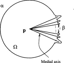
Then it is easy to see that the pointpis in the medial axis of Ω and that there are infinitely many segments in the medial axis of Ω emanating fromp.(Such pointpis an ∞-prong point in the language ofDefinition 3 below.)
Example 2: Let Ω be the domain whose boundary consists of two C∞ curves7 and 5, where γ is a portion of the boundary of a stadium like shape and δ is a curve represented by
for sufficiently small |t|, and γand δ are joined in such a way to form a closed C∞ curve, as shown in Figure 19.3.
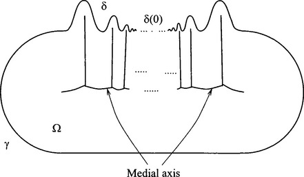
Then it is easy to see that the medial axis of Ω has infinitely many bifurcation points.
19.2.2 Medial axis transform
Now we define the medial axis and the medial axis transform.
Let Br(p) denote the closed disk of radius r centered at p.We define the set D(Ω) by
That is, D(Ω) is the set of all disks contained in Ω.
The core of a domain Ω is the set of all maximal disks in Ω, that is,
A disk Br(p) in CORE(Ω) is called a maximal disk, and in this case ∂Br(p) is called a maximal circle or contact circle.
Definition 1 (Medial axis and medial axis transform): The medial axis of a domain Ω is the set of all centers of disks in CORE(Ω). That is,
The medial axis transform of a domain Ω is the set of all ordered pairs of centers and radii of disks in CORE(Ω). That is,
Remark 1: In this case, we allow r = 0 and consider Br(p) as {p}. Such cases occur exactly at the sharp corners of ∂Ω.
A boundary point is a corner (point) if the unit tangent vector field is discontinuous at that point. It is called a sharp corner if the interior angle is strictly less than π, and a dull corner if the interior angle is strictly greater than π.
For a medial axis point p, B(p) denotes the disk Br(p) in CORE(Ω) with center p.
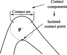
Definition 2: Let B(p) be a disk inCORE(Ω). Then we define the contact set ofp(or of B(p), or of ∂B(p)), denoted by C(p), as
A point in C(p) is called a contact point ofp(or of B(p), or of ∂B(p)). A connected component of C(p) is called a contact component ofp(or of B(p), or of∂B(p)).A contact component is called anisolated contact point if it is a point, and a contact arc if it is an arc containing its two end points. Finally, ∂B(p)is called acontact circle.
We note that a contact component is either an isolated contact point or a contact arc. Now we can characterize the medial axis points by the number of their contact components.
Definition 3: A pointpin MA(Ω), which is not a sharp corner point, is called an n- prong point (n ≥1), if C(p) has n contact components. We classify sharp corner points as 1-prong points[14]. An n-prong point pfor n ≥3 is called a bifurcation point. A 1-prong point is also called a terminal point.
Let(p, r) be inMAT(Ω). We call Br(p) a bifurcation disk ifpis a bifurcation point. In this case, ∂Br(p)is called a bifurcation circle. A disk B(p) ∈ CORE(Ω) is called an osculating disk at q∈ ∂Ω, if∂B(p)is an inscribed circle which osculates∂Ω atq.
In fact, around an n-prong point p(n ≥ 1), the medial axis MA(Ω) has exactly n‘prongs’ emanating from p.As we will see in section 19.2.4, this is a consequence of the graph structure of the medial axis (transform).
It is a fact that a terminal (i.e., 1-prong) point which is not a sharp corner is the center of an inscribed osculating circle, where an inscribed osculating circle of Ω is a circle contained in Ω which osculates ∂Ω at some point of ∂Ω. Also, it can be easily be shown geometrically that the curvature of ∂Ω takes a local maximum at an osculating point of an inscribed osculating circle. See Theorem 3.1 in [13] for a proof.
19.2.3 Finiteness results
From the real analyticity of the boundary of the domains in our class, we can derive some finiteness results about the medial axis (transform). First we require some definitions.
Definition 4: A 2-prong pointpin MA(Ω) is a generic 2-prong (point), if the following conditions are satisfied.
(1) The two contact components ofpare isolated contact points (denoted byq1andq2).
(2) Ifqi(i = 1,2) is not a dull corner, then ∂Ω nearqiis real analytic, and pis within the focal locus of a small piece of ∂Ω nearqi.
(3) Ifqi(i = 1, 2) is a dull corner, then ![]() is in a purely interior direction ofqi.
is in a purely interior direction ofqi.
See [13] for the definition of ‘being within the focal locus.’ Now we state the finiteness result.
19.2.4 Graph structure of medial axis transform
It has previously [13] been shown that the medial axis (transform) is path-connected. Furthermore, the medial axis (transform) of a domain has all the topological information of the original domain in the sense that:
Theorem 2 MA(Ω): is a strong deformation retract ofΩ, and in particular, MA(Ω)and MAT(Ω) are homotopic toΩ.
The main result [13] is that MA(Ω) and MAT(Ω) have the structure of the geometric graph. We call a set in ![]() 2(or in
2(or in ![]() 3) a geometric graph, if it is topologically a usually connected graph with a finite number of vertices and edges, where a vertex is a point in
3) a geometric graph, if it is topologically a usually connected graph with a finite number of vertices and edges, where a vertex is a point in ![]() 2(or in
2(or in ![]() 3) and an edge is a real analytic curve with a finite length, whose limits of tangents at the end points exist.
3) and an edge is a real analytic curve with a finite length, whose limits of tangents at the end points exist.
Theorem 3 (Graph structure of medial axis (transform)): MA(Ω) (MAT(Ω)) is a finite geometric graph.
In fact, MA(Ω) and MAT(Ω) are isomorphic as graphs, and besides the above theorem, we can obtain the following correspondence between the vertex degree of a point in MA(Ω) (MAT(Ω)) and the geometric property of that point. Let (p, r) be a point in MAT(Ω).
(1) If pis in an edge of MA(Ω), then pis a generic 2-prong, and thus MA(Ω) is real analytic at p(resp., (p, r)).
(2) If pis a vertex of degree 1 in MA(Ω), then pis either a sharp corner or the center of an inscribed osculating circle with one contact component.
(3) If pis a vertex of degree 3 or higher in MA(Ω), then pis a bifurcation point.
(4) If pis a vertex of degree 2 in MA(Ω), then pis a 2-prong which is not generic.
19.2.5 Domain decomposition lemma
In this section, we introduce our fundamental tool called the domain decomposition lemma which allows us to decompose a given domain into smaller and simpler subdomains so that the medial axis transform of the original domain is preserved as the union of the medial axis transforms of the subdomains. Using this domain decomposition lemma the medial axis transform is ‘localized’ so that, no matter how complicated the original domain is, its medial axis transform can be built out of simple building blocks which are easy to handle.
This technique makes it easy to analyze the mathematical properties of the medial axis transform. Moreover, since each building block is trivial to handle, the algorithm for finding the medial axis transform essentially boils down to bookkeeping for the domain decomposition procedure, which was greatly exploited by Choi et al. [14]. See Figure 19.5for an illustration of the basic idea of domain decomposition.
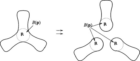
Theorem 4 (Domain decomposition lemma.): For any fixed medial axis pointp∈ MA(Ω), let B(p)(= Br(p)) be the corresponding maximal disk, i.e., B(p) ∈ CORE(Ω). Suppose A1, …, Anare the connected components ofΩB(p).Denote Ωi = Ai∪ B(p) for i = 1, …, n. Then
and
and
for every distinct i and j.
This lemma has been proved elsewhere [13]. The following definition describes the simplest building blocks out of which the entire MAT can be built.
19.3 ALGORITHMS
19.3.1 Piecewise linear and circular arc boundary
The first efficient algorithm for the computation of the medial axis was developed by Preparata [33]. However, it is restricted to convex domains with simple polygonal boundaries. Preparata’s algorithm for computing the medial axis of a convex polygon G may be described in two steps.
• (Reduction step) A sequence of convex polygons G = Gn, Gn-1, …, G4, G3are generated: each polygon Gi of the sequence is obtained from its predecessor Gi+1by an edge removal/vertex addition process. The criterion to determine which edge of the (i+1)-sided polygon Gi+1must be removed to yield the i-sided polygon Gi is given elsewhere [33]. Clearly, completion of the edge removal process always results in a triangle G3, whose medial axis may be trivially computed.
• (Construction step) The medial axes of the polygons G4, …, Gn are incrementally ‘updated’ from the medial axes of their predecessors by an edge addition/vertex removal process. The same edge that was removed from the polygon Gi+1during the edge removal process is now included in the polygon Gi.
The algorithm to update the medial axis of Gi+1from the medial axis of Gi during the edge addition/vertex removal process is presented in detail elsewhere [33]. Applying it iteratively, the medial axis of the original polygon Gn = G is computed. The running time of the algorithm has been shown to be O(n log n). A slightly modified algorithm, with a running time of O(n2), has also been suggested [33] for computing the medial axes of non-convex polygons.
In 1982, Lee presented [29] an O(n log n) algorithm for computing the medial axis of a planar shape represented by an n-edged simple (non-convex) polygon. Prior to this work, Kirkpatrick had presented [28] an asymptotically optimal O(n log n) algorithm for finding continuous skeletons of a set of disjoint objects. In fact Lee’s algorithm in [29] performed the computation of the Voronoi diagram of a simple polygon. Since one can obtain the medial axis of a simple polygon from its Voronoi diagram by removing the edges of the Voronoi diagram that connect to the reflex vertices (which is the dull corner in our language), computing the medial axis from the Voronoi diagram does not increase the time-complexity of the algorithm.
Basically, Lee’s approach was a divide and conquer. Let G be a simple polygon with vertices q1, …, qn and let ei denote the line segment ![]() . For each maximally contiguous sequence of reflex vertices qj, …, qk, he defined a chain of the edges of G as a sequence of elements ej-1,qj,ej,qi+1. …,qk-1,ek-1,qk,ek. His idea is to divide G into two lists G1and G2and thus recursively to construct the Voronoi diagrams VD(G1) and VD(G2), and then to merge both Voronoi diagrams to form the Voronoi diagram of G. Since the merging process takes O(n) time, the overall running time is O(n log n). In implementing this algorithm, he actually partitioned G into several chains C1, …, Ch. The reason for this was that the Voronoi diagram of a chain could be computed in time proportional to the number of elements in the chain. This result has been a basis of numerous algorithms dealing with polygonal boundary.
. For each maximally contiguous sequence of reflex vertices qj, …, qk, he defined a chain of the edges of G as a sequence of elements ej-1,qj,ej,qi+1. …,qk-1,ek-1,qk,ek. His idea is to divide G into two lists G1and G2and thus recursively to construct the Voronoi diagrams VD(G1) and VD(G2), and then to merge both Voronoi diagrams to form the Voronoi diagram of G. Since the merging process takes O(n) time, the overall running time is O(n log n). In implementing this algorithm, he actually partitioned G into several chains C1, …, Ch. The reason for this was that the Voronoi diagram of a chain could be computed in time proportional to the number of elements in the chain. This result has been a basis of numerous algorithms dealing with polygonal boundary.
Lee’s algorithm [29] cannot compute Voronoi diagrams of multiply-connected polygonal domains. Two algorithms have been independently developed by Held [26] and by Srinivasan and Nackman [45] for this purpose. While Held’s algorithm is capable of handling multiply-connected domains bounded by piecewise linear and circular segments, the algorithm developed by Srinivasan and Nackman can only accommodate polygons with a finite number of interior polygonal holes. Both of these methods are extensions of Lee’s algorithm, and they employ a similar divide-and-conquer strategy, which may be summarized as follows:
(1) Compute the interior Voronoi diagram of the outer boundary, neglecting the presence of the inner boundaries. This may be accomplished by Lee’s algorithm.
(2) Sort the inner boundaries into a decreasing order determined by the y-coordinate of the topmost vertex of each inner boundary.
(3) For each of the inner boundaries (in sorted order):
(a) Compute the exterior Voronoi diagram of the inner boundary, neglecting the presence of all the outer boundaries.
(b) Compute the ‘merge’ curve between the Voronoi diagram of the inner boundary and the merged Voronoi diagram computed thus far.
(c) Discard edges of the ‘old’ Voronoi diagrams that do not belong to the ‘new’ Voronoi diagram.
The merge curve in Step 3b is basically the contiguous set of edges of the new Voronoi diagram which did not exist in the old one. We also note that an extension of Lee’s algorithm is necessary to execute Step 3a, since the ′exterior′ Voronoi diagram of the inner boundaries needs to be computed.
19.3.2 Domains with free-form boundaries
Chou [15] was the first to develop an algorithm for computing the Voronoi diagram of a curvilinear domain. In his approach terminal points of the Voronoi diagram are first located at the convex, i.e., sharp, corners and the centers of the interior osculating circles of the boundary curve. The edges of the Voronoi diagram are then traced as a sequence of bisector points for the appropriate boundary segments; the terminal points of the Voronoi diagram are chosen as the starting points of this tracing scheme. The algorithm may also be extended to compute the Voronoi diagram of the region exterior to the boundary.
Farouki et al. [18–21] and Ramamurthy et al. [35–38] also made a great contributions to the development of both theory and algorithms for computing Voronoi diagrams and medial axes of planar domains with curvilinear (polynomial or rational) boundaries. Their studies can roughly be separated in two parts: the study of curve/curve bisectors and the study of general Voronoi diagram and medial axis algorithms.
Since the edges of Voronoi diagrams and medial axes are point/curve or curve/curve bisectors, algorithms for computing these bisector forms must be invoked by any construction algorithm. While an algorithm for computing generic point/curve bisectors (fora fixed point and a rational curve) was already available in literature, until then there existed no algorithm for computing the bisectors of pairs of rational curve segments.
Hence, the first important contribution of Farouki et al. and Ramamurthy et al. was the development of an algorithm for computing curve/curve bisectors. The important features of this algorithm are: (i) the bisectors of curved segments are directly computed without approximating the input curves; (ii) bisector segments having exact (rational) parameterizations are explicitly captured and represented in that form; (iii) bisector segments requiring approximation are guaranteed to have their geometric error (deviation from the exact curve) less than any prescribed tolerance; and (iv) tangent discontinuities of bisector loci are explicitly identified and included in their representation.
It has also been observed that certain degenerate bisector forms routinely arising in Voronoi diagram and medial axis constructions of planar domains cannot be accommodated by generic bisector algorithms. These include: (i) the bisector of a point and a curve in the case when the point lies on the curve; (ii) the bisector of a curve with itself (i.e., its self-bisector) and (iii) the bisector of two curves having a common endpoint. Owing to the complex nature of these degenerate bisector forms, substantial theoretical advances over the generic-case bisector algorithms have been necessary.
Farouki et al. and Ramamurthy et al. also developed theory and algorithms for computing Voronoi diagrams and medial axes of planar domains with curvilinear boundaries. As part of these theoretical developments, the precise relationship and differences between Voronoi diagrams and medial axes was also fully explored. To construct topologically faithful Voronoi diagrams and medial axes, methods to compute the exact coordinates of the bifurcation or branch points of Voronoi diagrams and medial axes are required. Toward this end, a thorough classification of the different types of bifurcation points that may be present in the Voronoi diagrams and medial axes of planar domains was given [19–21],[35–38], and the numerical schemes required to compute the exact coordinates of the bifurcations of each type was discussed.
19.3.3 Global decomposition algorithm
Most algorithms for finding the medial axis are local, in the sense that they first attempt to find the curve/curve bisectors and then try to join them together where they meet. This is a common thread in all of the algorithms described above.
In this subsection, we now describe the algorithm developed by Choi et al. [14]. For the lack of a suitable name, let us call it the global decomposition algorithm. Its overriding philosophy is quite different from the algorithms described above. First of all, it is global in nature: the main forte of this algorithm is its use of the domain decomposition lemma to decompose the original domain, no matter how complicated it is, so that it eventually becomes a collection of simple subdomains, called fundamental domains. If the original domain is subdivided for enough, then each fundamental domain becomes very simple, meaning that its medial axis transform is free of bifurcation points, and hence it is a real analytic curve. For this kind of fundamental domain, many curve/curve bisector algorithms are suitable for accurate computation of the medial axis (transform). For free-form curves, the algorithm proposed by Farouki et al. [18–21] seems to be the best.
The crux of the global decomposition algorithm is a procedure that successively decomposes the subdomains and keeps track of its data, using an appropriate data structure andoperations on it. One important benefit of this algorithm is that computation is localized to each subdomain: whatever happens in each subdomain does not affect other subdomains. This increases the stability of the algorithm. Since the medial axis transform of a domain with a free-from boundary is not a rational object, it is impossible to express it analytically. So one must try to obtain a good approximate medial axis transform. This is achieved by successively inserting circles so that the insertion of each circle becomes a domain decomposition step whose basic procedure is summarized as follows:
• Killing homology effectively makes the domain simply connected for the purpose of the algorithm.
• Divide the original domain into smaller and simpler domains and organize the data in such a way that the data structure makes transparent the existence of necessary bifurcation circles, inscribed osculating circles, etc., each of which requires a special algorithm.
• Compute an approximate medial axis transform by employing suitable curve/curve bisector algorithms.
• Using the above approximate medial axis transform data, run the recovery procedures for the medial axis transform and the boundary for each subdomains. If the error is within tolerance, the subdomain is left alone. Otherwise, decompose further the subdomain where the error is the greatest.
• Domain decomposition and recovery procedures are guaranteed to stop at finite steps because of various finiteness theorems.
The finiteness results in Theorem 1guarantees that this algorithm eventually terminates in finite steps in the sense that the domain is decomposed into fundamental domains each of which satisfies the error bound criterion. In the above, the killing homology procedure is a device to treat a multiply-connected domain as if it were simply-connected. More detail is given by Choi et al. [14].
We now briefly describe the data structure. The basic scheme is that each maximal circle is denoted by a vertex or a node of a graph, and the edges of the graph are formed according to the usual adjacency rule. The diagram on the left in Figure 19.6denotes a subdomain, possibly a fundamental domain, and the diagram on the right represents part of the graph where the two nodes correspond to the two circles and the edge connecting them signifies the subdomain bounded by these two circles. Figure 19.7represents a similar situation. The difference here is that the osculating circle (labelled ‘2’) represents a terminal node, i.e., the vertex of degree 1 in the graph.
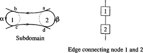

Figure 19.8 shows a quite different picture. In this example, the node marked ‘V’ does not correspond to any circle in the domain. However, by a topological argument, the domain bounded by the three circles 1, 2, and 3 must contain a bifurcation point (circle). The problem here is that, although the existence of a bifurcation point is guaranteed, it has not yet been found. Our algorithm is designed to detect the existence of such implied bifurcation points, and in Figure 19.8 it is marked V to signify that it is a virtual node.
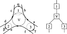
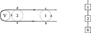
Figure 19.9represents a similar situation except that in this case the virtual node has to be a terminal node.
The overall performance of the algorithm is illustrated in Figures 19.10to 19.17. Figure 19.10 shows a given domain, and Figure 19.11 shows the stage reached by algorithm after several circles have been inserted. Its corresponding graph is given in Figure 19.12. In Figure 19.13, several more circles are inserted, and Figure 19.14 shows the recovered domain drawn on top of the original domain. In this illustration, domain recovery is simply performed by using the quadratic curves obtained from the contact data of the circles. Figure 19.15 shows a case where yet more circles have been added, and Figure 19.16 shows the recovered domain drawn on top of the original domain; in this case the domains look identical. Figure 19.17 shows the medial axis computed this way.
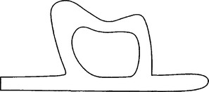
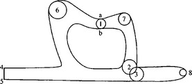
Figure 19.11 The domain of Figure 19.10 with a few circles inserted.
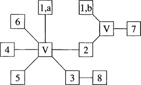
Figure 19.12 The data structure corresponding to Figure 19.11.
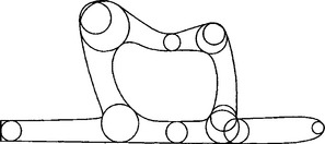
Figure 19.13 The domain of Figure 19.10 after several more circles have been inserted.
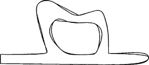
Figure 19.14 The domain of Figure 19.11 recovered using the data shown in Figure 19.13.
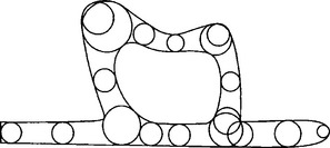
Figure 19.15 The domain of Figure 19.11 with further circles added.
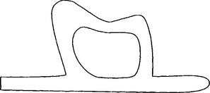
Figure 19.16 The domain of Figure 19.11 recovered using the data in Figure 19.15.

Figure 19.17 The domain of Figure 19.11 and its medial axis.
The global decomposition algorithm has been used in practical applications for many years, and we have found it to perform very robustly.
19.4 CONCLUDING REMARKS
We conclude this chapter by commenting on some important developments not mentioned above.
One important area not very well understood is the medial axis transform of a general three-dimensional domain. It is in general very difficult to understand and is perhaps prohibitively expensive to describe so that no one was able to come up with a complete and mathematically rigorous treatment. But there are some progress: Sherbrooke et al. [42],[43] developed an algorithm for general three-dimensional polyhedral solids of arbitrary genus without cavities, with non-convex vertices and edges. Their algorithm is based on a classification scheme which relates different pieces of the medial axis to one another even in the presence of degenerate medial axis points. Wolter [51] showed that the ‘cut locus’ concept offers a common framework lucidly unifying, regardless of dimension, different concepts such as Voronoi diagrams, medial axes and equidistantial point sets.
Since its inception in the 1960s in the biological sciences, the medial axis transform has been quite useful in compactly representing the information of shapes ranging from crude bitmap images to general Riemannian manifolds. A salient topic in this regards is the ‘inverse’ problem of the medial axis transform, i.e., the boundary regeneration of the shape from its medial axis transform. Vermeer [47] provided the details for the conversion of the medial axis transform of a set of two- and three-dimensional objects to a boundary representation. She demonstrated certain smoothness properties of the medial axis transform and showed the relationship between the tangent to the medial axis transform at a point and the boundary points related to that medial axis point. Amenta et al. [2],[3] introduced the ‘power crust’ algorithm to construct piecewise-linear approximations to both the object surface and the medial axis transform given an input point sample from the object surface. Their algorithm first uses the sample points to approximate the medial axis transform, and then apply an inverse transform to it to produce a piecewise-linear surface approximation.
There is a volume of literature on many other aspects of the medial axis transform. For example, there are a lot of works in the application of the medial axis transform to the mesh generation in the finite element method in numerical analysis. Another example isthe so-called skeleton of the bitmap image which is essentially the same as the medial axis transform in the context of bitmap image [23].
1. Vancouver, B.C. Alt, H., Schwarzkopf, O., The Voronoi diagram of curved objects. Proc. of the 11th ACM Comput. Geom. Symp. 1995:89–97.
2. Amenta, N., Choi, S., Kolluri, R., The power crust. Proceedings of 6th ACM Symposium on Solid Modeling. 2001:249–260.
3. Amenta, N., Kolluri, R., The medial axis of a union of balls. Canadian Conference on Computational Geometry. 2000:111–114.
4. Armstrong, C.G., Tam, T.K.H., Robinson, D.J., Mckeag, R.M., Price, M.A. Automatic generation of well structured meshes using medial axis and surface subdivision. In: Gabriele G.A., ed. Advances in Design Automation. New York: ASME; 1991:139–149.
5. August Badler, N.L., Dane, C., The medial axis of a coarse binary image using boundary smoothing. Proc. Pattern Recognition and Image Processing. 1979:286–291.
6. Cambridge, MA Blum, H. A transformation for extracting new descriptors of shape. In: Wathen-Dunn W., ed. Models for the Perception of Speech and Visual Form. MIT Press; 1967:362–380.
7. Blum, H. Biological shape and visual science (part I). J. Theor. Biol. 1973;38:205–287.
8. Blum, H., Nagel, R.N. Shape description using weighted symmetric axis features. Pattern Recog. 1978;10:167–180.
9. Brandt, J.W. Theory and Application of the Skeleton Representation of Continuous Shapes. PhD thesis, Univ. of California, Davis, CA. 1991.
10. June Brandt, J.W., Jain, A.K., Algazi, V.R. Medial axis representation and encoding of scanned documents. J. Visual Commun. Image Represent. 1991;2:151–165.
11. Chiang, C.S. The Euclidean Distance Transform. PhD thesis, Purdue University. 1992.
12. Choi, H.I., Choi, S.W., Han, C.Y., Moon, H.P., Roh, K.H., Wee, N.-S. New algorithm for offset of plane domain via MAT. In: Differential and Topological Techniques in Geometric Modeling and Processing ’98. Bookplus Press; 1998:161–185.
13. Choi, H.I., Choi, S.W., Moon, H.P. Mathematical theory of medial axis transform. Pacific J. Math. 1997;181:57–88.
14. Choi, H.I., Choi, S.W., Moon, H.P., Wee, N.-S., New algorithm for medial axis tranform of plane domain. Graph. Models and Image Proc, 1997;59:463–483.
15. Chou, J.J. Numerical Control Milling Machine Toolpath Generation for Regions Bounded by Free Form Curves. PhD thesis, University of Utah. 1989.
16. Chou, J.J. Voronoi diagrams for planar shapes. IEEE Comput. Graph. Applic. 1995;15(3):52–59.
17. Dirichlet, G.L. Über die reduktion der positiven quadratischen Formen mit drei unbestimmten ganzen Zahlen. J. of Reine Angew, Math. 1850;40:209–227.
18. Farouki, R.T., Johnstone, J.K. The bisector of a point and a plane parametric curve. Computer Aided Geometric Design. 1994;11:117–151.
19. Farouki, R.T., Johnstone, J.K. Computing point/curve and curve/curve bisectors. In: Fisher R.B., ed. Design and Application of Curves and Surfaces (The Mathematics of Surfaces V). Pohang, Korea: Oxford University Press; 1994:327–354.
20. Farouki, R.T., Ramamurthy, R. Degenerate point/curve and curve/curve bisectors arising in medial axis computations for planar domains with curved boundaries. Computer Aided Geometric Design. 1998;15:615–635.
21. Farouki, R.T., Ramamurthy, R. Specified-precision computation of curve/curve bisectors. Int. J. Comput. Geom. Applic. 1998;8:599–617.
22. Gelston, S.M., Dutta, D. Boundary surface recovery from skeleton curves and surfaces. Computer Aided Geometric Design. 1995;12:27–51.
23. Gonzalez, R.C., Woods, R.E., Digital Image Processing. Addison-Wesley, 1992.
24. Gursoy, H.N. Shape Interrogation by Medial Axis Transform for Automated Analysis. PhD thesis, MIT. 1989.
25. Gursoy, H.N., Patrikalakis, N.M. An automatic coarse and fine surface mesh generation scheme based on the medial axis tranform, I: Algorithms. Engin. Comput. 1992;8:121–137.
26. Held, M. On the Computational Geometry of Pocket Machining. Springer; 1991.
27. C.M. Hoffmann and C.-S. Chiang. The medial axis transform for 2D regions. Preprint.
28. October Kirkpatrick, D.G., Efficient computation of continuous skeletons. Proc. 20th Annu. Symp. Found. Computer Sci. 1979:18–27.
29. Lee, D.T. Medial axis transformation of a planar shape. IEEE Trans. Pattern Anal. Machine Intell. 1982;PAMI-4:363–369.
30. Lee, D.T., Drysdale, R.L. Generalization of Voronoi diagrams in the plane. SIAM J. of Computing. 1981;10:73–87.
31. Persson, H. NC machining of arbitrarily shaped pockets. Computer-Aided Design. 1978;10:169–174.
32. Pizer, S.M., Oliver, W.R., Bloomberg, S.H. Hierarchical shape description via the multiresolution symmetric axis transform. IEEE Trans. Pattern Anal. Machine Intell. 1987;9:505–511.
33. Preparata, F.P., The medial axis of a simple polygon. Proc. 6th Symp. Math. Foundations of Comput. Sci. 1977:443–450.
34. Preparata, F.P., Shamos, M.I. Computational Geometry: An Introduction, Second Edition. Berlin: Springer; 1988.
35. Ramamurthy, R. Voronoi Diagrams and Medial Axes of Planar Domains with Curved Boundaries. PhD thesis, University of Michigan. 1998.
36. Ramamurthy, R., Farouki, R.T. Topological and computational issues in Voronoi diagram and medial axis constructions for planar domains with curved boundaries. In: Differential and Topological Techiniques in Geometric Modeling and Processing ’98. New York: Bookplus Press; 1998:1–26.
37. Ramamurthy, R., Farouki, R.T. Voronoi diagram and medial axis algorithm for planar domains with curved boundaries I: Theoretical foundations. J. Comput. Appl. Math. 1999;102(1):119–141.
38. Ramamurthy, R., Farouki, R.T. Voronoi diagram and medial axis algorithm for planar domains with curved boundaries II: Detailed algorithm description. J. Comput. Appl. Math. 1999;102(2):253–277.
39. Shaked, D., Bruckstein, A.M. Pruning medial axes. Comput. Vis. Image Understanding. 1998;69:156–169.
40. Sheehy, D.J., Armstrong, C.G., Robinson, D.J. Shape description by medial surface construction. IEEE Transactions on Visualization and Computer Graphics. 1996;2(1):62–72.
41. Sherbrooke, E.C. 3-D Shape Interrogation by Medial Axis Transform. PhD thesis, MIT. 1995.
42. May Sherbrooke, E.C., Patrikalakis, N.M., Brisson, E., Computation of medial axis transform of 3-D polyhedra. Proceedings of the Third A CM Solid Modeling Conference. 1995:187–199.
43. Sherbrooke, E.C., Patrikalakis, N.M., Brisson, E. An algorithm for the medial axis transform of 3D polyhedral solids. IEEE Transactions on Visualization and Computer Graphics. 1996;2:44–61.
44. Sherbrooke, E.C., Patrikalakis, N.M., Wolter, F.E., Differential and topological properties of medial axis transforms. Graph. Models and Image Proc, 1996;58:574–592.
45. Srinivasan, V., Nackman, L.R. Voronoi diagram for multiply-connected polygonal domains I: Algorithm. IBM J. Res. Develop. 1987;31:361–372.
46. Tarn, T.K.H., Armstrong, C.G. 2D finite element mesh generation by medial axis subdivision. Adv. Engin. Software. 1991;13:313–324.
47. Vermeer, P.J. Medial Axis Transform to Boundary Representation Conversion. PhD thesis, Purdue University. 1994.
48. Voronoi, G.M. Nouvelles applications des paramètres continus à la théorie des formes quadratiques. J. Reine Angew. Math. 1908;134:198–287.
49. Wolter, F.E. Distance function and cut loci on a complete Riemannian manifold. Arch. Math. 1979;32:92–96.
50. Wolter, F.E. Cut Locus in Bordered and Unbordered Riemannian Manifolds. PhD thesis, Tech. Univ. of Berlin. 1985.
51. January Wolter, F.E., Cut locus and meidal axis in global shape interrogation and representation. MIT Ocean Engineering Design Laboratory Memorandum 92-2. 1992.
52. Yap, C.-K. An O(n log n) algorithm for the Voronoi diagram of a set of simple curve segments. Discrete Comp. Geom. 1987;2:365–393.