Vector and Tensor Field Visualization
27.1 INTRODUCTION
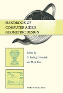
“Visualization transforms data into images that efficiently and accurately represent information about the data” [49, p.83]. This definition describes the visualization task as a transformation process like the one in Figure 27.1.
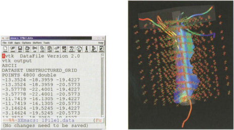
Figure 27.1 Visualization transforms data into images. Here, tensor data together with geometry is transformed into a computer generated image.
It is obvious on one side that one needs knowledge about the data and its underlying context to do the job. On the other side, it is necessary to use the whole repertoire of image generation to be efficient and accurate as the definition demands. In this chapter, we understand visualization as transformation of digital, numerical data into digital images by using computer graphics. This kind of visualization has been formed into a scientific discipline by a report of McCormick and DeFanti [34]. If you are looking for an example of classical visualization techniques, Merzkirch [35] provides an excellent survey on experimental flow visualization. The data in our applications stems from natural scientists or engineers doing measurements during experiments, observing natural or technical phanomena or simulating experiments by numerical calculations. The information about the data serves three main purposes [45], namely
• to get an impression of the experiment or simulation;
All three perposes are directed towards the natural scientist or engineer, so visualization is an inherent interdisciplinary endeavour from the perspective of a computer scientist. In the natural and engineering sciences, three types of numerical variables make up nearlyall numerical data: scalars, vectors, and tensors. Typical examples for scalar variables are temperature, pressure, density, and electrical charge. Vector variables are velocity, vorticity, magnetic field, electric field, force, and any kind of scalar gradient like temperature gradient. Tensor variables describe for example stress, strain or rate of deformation (in fluids). There are a lot of good visualization concepts for scalar data like colorimng, height fields, conturing, and volume visualization, but we like to concentrate in this chapter on vector and tensor data. A practical description of all kinds of visualization algorithms can be found in [49].
27.2 VISUALIZATION PROCESS
The transformation of data into images is a process with three steps, usually described as a visualization pipeline. A typical model is given by the three intermediate steps in Figure 27.2. The data generation phase stands outside the visualization process. Itmeans the creation of numerical data by simulation, measurements during experiments or observation of natural phanomena. The data enrichment and enhancement phase modifies the data to reduce its amount or improve the information content. Domain transformations, interpolation, sampling, and noise filtering are typical operations in this phase. The visualization mapping section is the heart of the whole transformation. The application data is mapped to visual primitives and attributes. This chapter will give an overview of successful techniques for vector and tensor data. The rendering phase does the usual computer graphics operation of creating an image on the screen from the graphics primitives and attributes combined with a camera model, lighting operations, anti-aliasing filtering, and hidden surface removal. Finally, the display phase shows the image on the screen or prints it on paper.
27.3 DATA SET TYPES AND INTERPOLATION METHODS
The data sets in visualization consist usually of two parts. The first part contains the grid and the second part data values associated with the grid. In our case the data values will always be vectors or tensors. The types of the data sets are not determined by the visualization process, but by the data generation process. This is an important issue for every visualization that takes places, especially since the data is usually discrete and an interpolation has to take place for all but the simple point-based direct visualization methods.
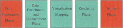
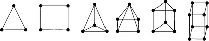
In numerical simulations, two types of algorithms still produce most of the data, finite difference and finite element methods. Both create a set of points, vertices, and associate the data in most cases with these points. Besides this, a grid consisting of a large number of cells is created. Each cell contains a small number of vertices. The cells do not intersect except at their boundaries and all cells fill the domain of the simulation. Finite difference methods prefer regular grids like cartesian and rectilinear grids, sometimes deformed into so-called structured grids by a mapping from a cartesian computational domain into the physical domain where the simulation is defined. Figure 27.3 gives a typical example. Finite element methods are more flexible, since they allow different kinds of cells in onesimulation and are able to fill complex geometries with cells. Typical cell types are given in Figure 27.3. A grid is called unstructured, if the cell neighbors are not given implicitby the indexing of the cells as it is possible for example for cartesian grids. There is a large variety of interpolation functions available, most often coupled with the cell types. Surveys on this topic are found in introductionary texts on finite element methods [3],[37]. Grid types in numerical simulations can be a lot more complicated by overlapping grids, several grid blocks with different grid types and multilevel techniques. A nice survey about grid types is given by [21]. Data sets from measurements or experiments are often regular since they are the result of image-generating processes like computer tomography (CT). If they come from other sources, scattered data is a typical type. Before a visualization can take place, one has to do scattered data interpolation. A description of this research area can be found in the chapter on Scattered Data Techniques in this handbook.
27.4 DIRECT MAPPINGS TO GEOMETRIC PRIMITIVES
The easiest way to create a visualization with the computer is to map the data values to geometric primitives. These primitives are collected into a scene that is presented by standard computer graphics techniques. If you are not familiar with computer graphics, you may consult a computer graphics textbook [17]. These direct visualization methods can be distinguished by the domain of information that each primitive represents. We will discuss point-based, line-based, surface-based, and volume-based methods in this section.
27.4.1 Point-based methods
Vectors and tensors are mathematical constructions with a strong physical background, so many elementary techniques show this heritage. The easiest techniques are hedgehogs. At one or more positions, usually where the discrete data is given, one shows a single graphical primitive representing the vector or tensor. For vectors, arrows are the common choice as in the left image of Figure 27.4.1. For symmetric tensors, tripods of the orthogonal eigenvectors give one typical way as can be depicted from the right image in Figure 27.4.1. Since the length of the three line segments can only indicate the absolute value of the eigenvectors, color is used to indicate the sign of the eigenvalues. Here, red indicates positive eigenvalues and green stands for negative eigenvalues. In case of only positive eigenvalues, ellipsoids are another typical choice. Glyphs give only information aboutthe data at a point. It is possible to include also gradient information. The local flow probe [13] gives a nice example by including the local streamline with curvature, torsion, divergence, and curl in the presentation of the vector data.
27.4.2 Line-based methods
This second kind of methods has an one-dimensional spatial domain. For vector fields, they are all based on integral curves. Let
be a d-dimensional, steady vector field over a domain D as in section 3. An integral curve of v through a ∈ D,
fulfils the two conditions
The calculation is typically based on a numerical method for ordinary initial value problems, like Euler method, Midpoint-Rule, Runge-Kutta-Fehlberg methods or Predictor-Corrector methods [46], sometimes with adaptive stepsize control to maintain given error bounds. Therefore, one calculates points on the curve which can be connected by line segments or small tube elements which leads to pictures like Figure 27.4.2. If one wants to include neighboring information in three-dimensional vector fields, one can compute a second close streamline to form a ribbon [6]. This can be improved by calculating the curvature of the streamline [61], since the two streamlines of the ribbon may diverge. The stream polygon [50] provides another concept for including information about a three-dimensional vector field along an integral curve. By rotating and shearing the polygon, one can visualize rotation and rate of deformation, for example in fluid flows. Very nice visualizations of integral curves can be generated by using an illumination model for curves. This has been demonstrated by Zöckler, Stalling and Hege [64]. Nielson and Jung [38] give an overview over efficient techniques for the computation of integral curves over tetrahedral meshes that allow an exact solution of the problem if linear interpolation is used. The formulation in barycentric coordinates simplifies the calculations in this case.
In the tensor field case, Dickinson [16] introduced the concept of a tensor line which corresponds to the integral curves of vector fields. Let

be a symmetric tensor field over the domain D. At each position x ∈ D, there are in general d real eigenvalues λ1 > … > λd and d orthogonal eigenvectors e1,…,ed with T(x)ei = λ iei. This defines d eigenvector fields

A tensor line of the i-th eigenvector field of T through b ∈ D is a curve d: (γ, δ) →D, t![]() d(t),γ<0<δ with the following two conditions:
d(t),γ<0<δ with the following two conditions:
i.e. the tangent of d is at every position parallel to the i-th eigenvector. Since this definition is far less known than than the integral curves above, Figure 27.4.2 illustrates this idea in two dimensions. Besides steady data, there is also unsteady data. Usually, one will be given data at discrete timesteps with fixed or moving positions as mentioned in section 27.3. From experimental flow visualization techniques, one has copied four different line-type methods [28],[29]. Let
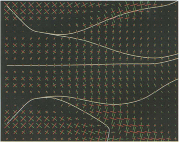
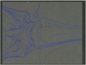
Figure 27.7 Tensor lines indicate the direction of maximum, medium or minimum forces, stress or strain. In this example, the tensor lines follow the maximum rate of strain.
be an unsteady vector field. A pathline of v through a ∈ D at ![]() is a curve
is a curve ![]() with the conditions
with the conditions
A pathline models the movement of a particle in the field (for example a positively charged particle in an electrical field). For velocity fields in fluid flows, one uses also timelines and streaklines.
A timeline is created by starting a line of colored dye particles in a windtunnel at one moment and tracing it by photographs. Mathematically, a timeline at time ![]() of v defined by a curve c : R ⊃ I → Rd at timestep τ0 is a curve
of v defined by a curve c : R ⊃ I → Rd at timestep τ0 is a curve
where
is a pathline of v through c(σ) at times τ0.
A streakline arises by inducing continously dye into a fluid flow from a fixed position. More formal, a streakline of v through a point a ∈ D is a curve
where
is a pathline of ν through a at time τ. Besides these two special cases for fluid dynamics, one uses also instantaneous integral curves in unsteady vector field visualization, i.e. integral curves of the vector fields
especially τ=τ0,…τn. Interestingly, there has not been much research on the line-type time-dependent methods for tensor fields.
27.4.3 Surface and volume-based methods
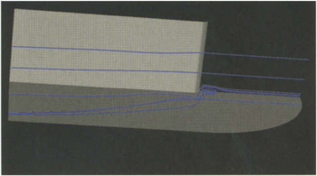
Besides point-based and line-based methods, several people have also tried surface and volume-based approaches. Computational Fluid Dynamics (CFD) is again a dominant application area. From there, the idea of a stream surface has been taken by Hultquist [26]. Let v : R3 → R3, x ![]() v(x) be a steady vector field. A stream surface S of v defined by a curve c : [α, β] → R3, σ
v(x) be a steady vector field. A stream surface S of v defined by a curve c : [α, β] → R3, σ ![]() c(σ) is a map
c(σ) is a map
with
In other words, a stream surface consists of all integral curves of v defined by the points on a continuous curve. Hultquist’s algorithm traces several integral curves from points on the defining curve and interpolates between them by triangles. If two neighboring integral curves become closer than a threshhold, he stops one of the traces. If two neighboring integral curves diverge, he introduces an additional trace to keep the triangles (and theerror) small. Van Wijk [60] has published a different algorithm based on local implicit surface pieces. There is less experience with surface techniques for tensor fields so far.
There are only a few volume-based visualization techniques for vector fields and tensor fields. We mention tridimensional line integral convolution (3D LIC) in the section about texture-based methods. Some people have applied sucessful scalar data methods like volume rendering on vector fields. An early example based on filters and textures has been presented by Crawfis and Max [9]. It uses textures to create the impression of a large number of moving short line segments (arrows, splats) in the volume. It can also be seen as a texture-based technique. Several people have looked at using volume graphics approaches to vector fields, usually using derived scalars like components, magnitude or rotation magnitude, see Crawfis et al. for a nice example [10]. There are also successful attempts to use a large number of particles moving in a vector field creating virtual smoke [33],[24].
27.5 ATTRIBUTE MAPPINGS
Besides the mapping to geometric primitives, one can also use attributes of computer graphics primitives to visualize the data. Color is probably the oldest attribute, but it is not easy to use for vector or tensor data, if one wants to show the whole data and not only a derived scalar like magnitude or component. Other attributes offer better possibilities. Texture is a well-known standard computer graphics method to show fine details without geometric modeling of the detail information. Essentially, it is the mapping of a picture on geometry, typically polygons. It was first developed by Catmull [8]. The maximal information content of textures with respect to the screen resolution make them attractive for visualization purposes. Spot noise by van Wijk [59] is an early example. The basic underlying idea is that a large number of particles leads to textures because the individual particles can not be distinguished. For the visualization of vector fields, small, randomly placed ellipsoids are used with eccentricity proportional to the magnitude and the longer axis aligned with the vector direction. Spot noise influenced the most popular texture based visualization algorithm, line integral convolution (LIC), invented by Cabral and Leedom [7]. LIC starts with a white noise texture of grey values and smears the grey values along the integral curves. This enhances the color correspondence in the direction of the vector field and leads to nice vector field visualizations, see Figure 27.5. The smearing effect is created by convoluting the pixel values along the integral curves. Stalling and Hege [53] have given a very fast and efficient implementation which is often used in applications. A comparison of LIC and sport noise has been published by de Leeuw and van Liere [11]. Due to its success for steady fields on rectilinear grids, many people have tried to extend LIC to other data set types. Forssell and Cohen discuss curvilinear surfaces [18], Battke et al. arbitrary surfaces [5]. Several people have worked on animation of textures and dye (color) advection to apply LIC to unsteady vector fields. Shen, Johnson, Ma [51] use color to animate the texture. The convolution filter can also be used, as is demonstrated by the unsteady flow line integral convolution (UFLIC) algorithm by Shen and Kao [52]. The application of LIC to three-dimensional vector fields has been tried by several authors, but due to the complexity of three-dimensional textures, this is a difficult endeavour. One needs a lot of hints for the eyes and research into perceptionis necessary to find good tricks to do this. Interrante et al. have done research in this direction [27].


27.6 STRUCTURE AND FEATURE BASED MAPPINGS
Visualization creates meaningful images to the user to understand his data. Since the whole data is in digital form, it makes sense to use the computer to look for structure elements and specific features, once a precise definition is given. For vector and tensor fields, topology provides a clearly defined mathematical framework with high application relevance. Topology extraction and visualization is therefore a good way to concentrate information about the data or enhance the presentation to the scientist or engineer working with the data. We review the history and state of the art in the first two subsections. For many interesting aspects of data sets, there are mathematical formulations, often many with partly contradicting content. These formulations can be taken as basis for feature extraction algorithms. The results of these algorithms are visualized. Examples are given in the last subsection.
27.6.1 Vector field topology
Integral curves of steady, Lipschitz-continuous vector fields as introduced in section 27.4.2 exist through every point and are unique. This follows from the well-known Picard-Lindelöf theorem of ordinary differential equations. Therefore, the whole domain is filled with curves, so one can analyze the topological behavior of all these curves. The general idea of topological methods is to group all curves together that can be continuously deformed into each other. Such curves all called homotop in topology. The first step is to identify all potential start and end points (sets) of integral curves. More formally, let ca : R → D be an integral curve through a ∈ D of a vector field v : Rd ⊃ D → Rd. The α-limit set of ca is the set
(![]() denotes the closure of the domain D.) The most popular case for A or Ω is a critical point {p} with v (p) = 0. Points of the domain boundary ∂ D can also act as α- or ω-limit set. Further possibilities are closed integral curves, tori and so-called strange attractors/repellors that do not fit into the other categories. These results belong to the theory of dynamical systems. An excellent comic-style introduction is given by Abraham and Shaw [1], more formal texts are also available [25],[20].
denotes the closure of the domain D.) The most popular case for A or Ω is a critical point {p} with v (p) = 0. Points of the domain boundary ∂ D can also act as α- or ω-limit set. Further possibilities are closed integral curves, tori and so-called strange attractors/repellors that do not fit into the other categories. These results belong to the theory of dynamical systems. An excellent comic-style introduction is given by Abraham and Shaw [1], more formal texts are also available [25],[20].
If all potential α- and ω-limit sets are found, the boundaries of the regions consisting of homotop curves are calculated. These curves in two dimensions resp. surfaces in three dimensions are called separatrices. Details on their computation can be found in the articles cited below. For two-dimensional vector fields, Helman and Hesselink did pioneer work in this area [22],[23]. They treated exclusively critical points. Nielson et al. give a nice description including the use of barycentric coordinates [40]. A clear treatment of the boundary can be found in an article by Scheuermann et al. [48]. Figure 27.6.1 illustrates the difference between the two approaches. The detection and analysis of closed integral curves has been finished by Wischgoll and Scheuermann just recently [62]. An example is presented in Figure 27.6.1. Since strange attractors and repellors do notappear in generic planar vector fields as a result of a famous theorem of Peixoto [44], the planar topology visualization is now complete for vector fields. In three dimensions, one has dealt with critical points alone without defining the separating surfaces that replace the separating curves from the two dimensional case [19]. Another aspect of topology visualization is the simplification of the topological structure. Especially in turbulentvelocity vector fields, the number of critical points and séparatrices is so high that a depiction of the field is difficult. Nielson et al. [39] used wavelet transforms of the vector field to reduce its structural complexity. This work has been extended to a nice treatment of wavelets over curvilinear grids [41] which opened the way for the use of multiresolution visualization techniques for this important class of data sets. De Leeuw and van Liere [12] simplified the topological graph consisting of critical points and separating points at the boundary as vertices and separatrices as edges using topology based rules without changing the underlying vector field. Tricoche, Scheuermann and Hagen [55] simplified the vector field topology by merging critical points into higher order critical points, see Figure 27.6.1. Lodha et al. [32] maintain the topology as long as possible while reducing the information content of the remaining vector field. Vector Field Topology can also be used to compare different flows. One needs a measure for the similarity of different topologies. Lavin, Batra and Hesselink have used the earth mover’s distance to compare the critical points in the field [30],[4].


27.6.2 Tensor field topology
The success of the vector field topology visualization led Delmarcelle and Hesselink [14] to analyze the structure of symmetric second-order tensor fields. The basic idea is exactly the same as for vector fields, one looks for homotop integral curves — in this case tensor lines. The role of the critical points is now filled by the so-called degenerate points. At these points, the tensor field has two equal eigenvalues, so there is no unique tangent given by the eigenvectors and one can not define a tensor line through these points. Separatrices can be defined again, but due to the difference between tangents and vectors (vectorsdefine an orientation), one gets different patterns, see Figure 27.6.2.
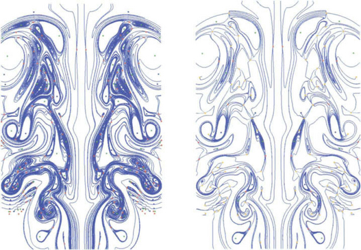
Figure 27.11 The topology of turbulent vector fields can be rather complicated. It is possible to scale the topology to allow a simpler depiction of large scale structures.
Lavin, Batra and Hesselink [31] extended some of these ideas to three dimensions, but as in the vector case, there is still no complete algorithm for tridimensional topology visualization of symmetric tensor fields. Tricoche, Scheuermann and Hagen [56] show the simplification of tensor field structure based on the fusion of degenerate points of higher order.
27.6.3 Feature detection algorithms
“A feature is defined as anything contained in a data set that might be of interest for interpretation” [47, p. 15]. This vague definition comes from the broad variation of application areas and the different measurement and simulation methods. The main point is that a feature must be local with respect to the data set domain, so that algorithms always try to find the domain feature. An excellent overview in the area of fluid flows is given by Roth in his recent Ph.D. thesis [47]. Delmarcelle and Hesselink [15] distinguish features by the dimension of the feature domain. This leads to point, line, surface and volume features. The critical and degenerate points from subsections 27.6.1 and 27.6.2 are typical examples for point features. Again, fluid flow applications dominate this research area up to now. Vortex cores [42],[2],[54],[36] are typical line features describing the“center” of a vortex in three dimensions. Shock fronts [43] are surface features where a physical property like pressure is not continous. It is often found by looking for high absolute values of the gradient. Volume features are often defined as all points with all points above or below a threshhold of a scalar function. This scalar function may be derived from a vector field like the absolute value of the vorticity vector field [63]. A general, application-independent approach based on these ideas to feature extraction and visualization has been shown by Post and Silver, together with several coworkers. It is mainly directed towards scalar fields, but it marks a way for further research for feature extraction in vector and tensor fields [57],[58].
1. Abraham, R.H., Shaw, C.D., Dynamics, the Geometry of Behavior I–IV. 1982, 1983, 1985. Aerial Press, 1988.
2. Washington, DC Banks, D., Singer, B., Vortex tubes in turbulent flows: Identification, representation, reconstruction. IEEE Visualization ’94. 1994:132–139.
3. Bathe, K.-J. Finite Element Procedures. Santa Cruz, CA: Prentice Hall; 1996.
4. San Francisco, CA Batra, R., Hesselink, L., Feature comparisons of 3D vector fields using earth mover’s distance. IEEE Visualization ’99. 1999:105–114.
5. Battke, H., Stalling, D., Hege, H.-C. Fast line integral convolution for arbitrary surfaces in 3D. In: Visualization and Mathematics. Upper Saddle River, NJ: Springer; 1997:181–195.
6. Bunning, P.G. Numerical algorithms in cfd post-processing. Technical Report Lecture Series 1989-07, van Karman Institute for Fluid Dynamics. 1989.
7. Cabral, B., Leedom, L.C. Imaging vector fields using line integral convolution. Computer Graphics, SIGGRAPH ’93. 1993;27(4):263–270.
8. December Catmull, E. A Subdivision Algorithm for Computer Display of Curved Surfaces. PhD thesis, Computer Science Department, University of Utah, Salt Lake City, UT. 1974.
9. Crawfis, R., Max, N. Direct volume visualization of three dimensional vector fields. In: Volume Visualization Workshop 1992. New York: ACM Siggraph; 1992:55–60.
10. Crawfis, R., Max, N., Becker, B. Vector field visualization. IEEE Computer Graphics and Applications. 1994;14(5):50–56.
11. de Leeuw, W.C., van Liere, R. Comparing LIC and spot noise. In: IEEE Visualization ’98. IEEE Computer Society Press; 1998:359–365.
12. de Leeuw, W.C., van Liere, R., Visualization of global flow structures using multiple levels of topology. EUROGRAPHICS – IEEE TCVG Symposium on Visualization. 1999:45–52.
13. de Leeuw, W.C., van Wijk, J.J. A probe for local flow field visualization. In: IEEE Visualization ’93. Los Alamitos, CA: IEEE Computer Society Press; 1993:39–45.
14. Delmarcelle, T., Hesselink, L. Visualizing second-order tensor fields with hyper-streamlines. IEEE Computer Graphics & Applications. 1993;13(4):25–33.
15. Delmarcelle, T., Hesselink, L. A unified framework for flow visualization. In: Gallagher R.S., ed. Computer Visualization: Graphics Techniques for Scientific and Engineering Analysis. Los Alamitos, CA: CRC Press, 1994.
16. Dickenson, R.R., A unified approach to the design of visualization software for the analysis of field problems. SPIE Proceedings. 1989:173–180.
17. Foley, J.D., van Dam, A., Feiner, S.K., Hughes, J.F. Computer Graphics – Principles and Practice, 2nd edition. Addison-Wesley; 1996.
18. Forssell, L.K., Cohen, S.D. Using line integral convolution for flow visualization: curvilinear grids, variable-speed animation, and unsteady flows. IEEE Transaction on Visualization and Graphics. 1995;1(2):133–141.
19. San Diego Globus, A., Levit, C., Lasinski, T., A tool for visualizing the topology of three-dimensional vector fields. IEEE Visualization ’91. 1991:33–40.
20. Guckenheimer, J., Holmes, P. Dynamical Systems and Bifurcation of Vector Fields. Reading, MA: Springer-Verlag; 1983.
21. Hamann, B., Moorhead, R.J., II. A survey of grid generation methodologies scientific visualization efforts. In: Scientific Visualization. New York: IEEE Computer Society; 1997:59–101.
22. Los Alamitos, CA Helman, J.L., Hesselink, L., Surface representations of two- and three-dimensional fluid flow topology. Nielson G.M., Shriver B., eds., eds. Visualization in Scientific Computing. 1990:6–13.
23. May Helman, J.L., Hesselink, L. Visualizing vector field topology in fluid flows. IEEE Computer Graphics and Applications. 1991;11(3):36–46.
24. Hin, A., Post, F. Visualization of turbulent flow with particles. In: IEEE Visualization ’93. Los Alamitos, CA: IEEE Computer Society Press; 1993:46–52.
25. Hirsch, M.W., Smale, S. Differential Equations, Dynamical Systems and Linear Algebra. Los Alamitos, CA: Academic Press; 1974.
26. Boston, MA Hultquist, J.P.M., Constructing stream surfaces in steady 3D vector fields. Kaufman A.E., Nielson G.M., eds., eds. IEEE Visualization ’92. 1992:171–178.
27. Interrante, V., Grosch, C. Visualizing 3D flow. IEEE Computer Graphics and Applications. 1998;18(4):49–53.
28. Lane, D.A. Visualization of time-dependent flow fields. In: IEEE Visualization ’93. New York: IEEE Computer Society Press; 1993:32–38.
29. Lane, D.A. Visualizing time-varying phenomena in numerical simulations of unsteady flows. Technical Report NAS-96-001, NASA Ames Research Center. 1996.
30. Research Triangle Park, NC Lavin, Y., Batra, R., Hesselink, L., Feature comparisons of vector fields using earth mover’s distance. IEEE Visualization ’98. 1998:103–109.
31. Lavin, Y., Levy, Y., Hesselink, L. Singularities in nonuniform tensor fields. In: Yagel R., Hagen H., eds. IEEE Visualization ’97. Los Alamitos, CA: IEEE Computer Society; 1997:59–66.
32. Salt Lake City, UT Lodha, S.K., Renteria, J.C., Roskin, K.M., Topology preserving compression of 2D vector fields. IEEE Visualization 2000. 2000:343–350.
33. Ma, K.-L., Smith, P.J. Virtual smoke: an interactive 3D flow visualization technique. In: Kaufman A.E., Nielson G.M., eds. IEEE Visualization ’92. Los Alamitos, CA: IEEE Computer Society Press; 1992:46–53.
34. Mccormick, B.H., Defanti, T.A. Visualization in scientific computing. Computer Graphics. 21(6), 1987.
35. Merzkirch, W. Flow Visualisation, 2nd Edition. Los Alamitos, CA: Academic Press; 1987.
36. Nagoya, Japan Miura, H., Kida, S., Identification of central lines of swirling motion in turbulence. Proceedings of Intl. Conference on Plasma Physics. 1996:866–869.
37. Mohr, G.A. Finite Elements for Solids, Fluids, and Optimization. New York: Oxford University Press; 1992.
38. Nielson, G.M., Jung, I.-H. Tools for computing tangent curves for linearly varying vector fields over tetrahedral domains. IEEE Transactions on Visualization and Computer Graphics. 1999;5(4):360–372.
39. Nielson, G.M., Jung, I.-H., Sung, J. Haar wavelets over triangular domains with applications to multiresolution models for flow over a sphere. In: Yagel R., Hagen H., eds. IEEE Visualization ’97. Oxford: IEEE Computer Society; 1997:143–149.
40. Nielson, G.M., Jung, I.-H., Sung, J., Srinivasan, N., Yoon, J.-B., Tools for Computing Tangent Curves and Topological Graphs. IEEE Computer Society Press: Los Alamitos, CA, 1997:527–562.
41. Nielson, G.M., Sung, J. Wavelets over curvilinear grids. In: IEEE Visualization ’98. Los Alamitos, CA: IEEE Computer Society Press; 1998:313–317.
42. Pagendarm, H.-G., Henne, B., Rütten, M. Detecting vortical phanomena in vector data by medium-scale correlation. In: IEEE Visualization ’99. Los Alamitos: IEEE Computer Society Press; 1999:409–412.
43. Pagendarm, H.-G., Seitz, B. An algorithm for detection and visualization of discontinuities. In: Palamidese P., ed. Scientific Visualization – Advanced Software Techniques. Los Alamitos: Ellis Horwood Ltd; 1993:161–177.
44. Peixoto, M. Structural stability on two-dimensional manifolds. Topology. 1961;2:101–121.
45. Post, F., van Walsum, T. Fluid flow visualization. In: Hagen H., Müller H., Nielson G.M., eds. Focus on Scientific Visualization. Springer; 1993:1–40.
46. Press, W.H., Teukolsky, S.A., Vetterling, W.T., Flannery, B.P. Numerical Recipes in C, 2nd Edition. Berlin: Cambridge University Press; 1992.
47. Roth, M. Automatic Extraction of Vortex Core Lines and Other Line-Type Features for Scientific Visualization. PhD thesis, ETH Zürich. 2000.
48. Scheuermann, G., Hamann, B., Joy, K.I., Kollmann, W. Visualizing local vector field topology. Journal of Electronic Imaging. 2000;9(4):356–367.
49. Schroeder, W., Martin, K.W., Lorensen, B. The Visualization Toolkit, 2nd Edition. Cambridge, UK: Prentice-Hall; 1998.
50. Los Alamitos, CA Schroeder, W., Volpe, C., Lorenson, W., The stream polygon: a technique for 3D vector field visualization. IEEE Visualization 1991. 1991:126–132.
51. Shen, H.-W., Johnson, C.R., Ma, K.-L. Visualizing vector fields using line integral convolution and dye advection. In: IEEE Symposium on Volume Visualization. Upper Saddle River, NJ: ACM; 1996:63–70.
52. Shen, H.-W., Kao, D.L. A new line integral convolution algorithm for visualizing time-varying flow fields. IEEE Transactions on Visualization and Computer Graphics. 1998;4(2):98–108.
53. Stalling, D., Hege, H.-C. Fast and resolution independent line integral convolution. Computer Graphics, SIGGRAPH ’95. 1995;29(4):249–256.
54. Sujudi, D., Haimes, R., Identification of swirling flow in 3D vector fields. 12th AIAA CFD Conference. AIAA Paper 95-1715, San Diego, CA. 1995.
55. Los Alamitos, CA Tricoche, X., Scheuermann, G., Hagen, H., A topology simplification method for 2D vector fields. IEEE Visualization 2000. 2000:359–366.
56. To appear Tricoche, X., Scheuermann, G., Hagen, H., Vector and tensor field topology simplification on irregular grids. Joint Eurographics and IEEE TCVG Symposium on Visualization 2001. 2001.
57. van Walsum, T., Post, F. Selective visualization of vector fields. Computer Graphics Forum, EUROGRAPHICS ’94. 1994;13(3):339–347.
58. van Walsum, T., Post, F.H., Silver, D., Post, F.J. Feature extraction and iconic visualization. IEEE Transactions on Visualization and Computer Graphics. 1996;2(2):111–119.
59. van Wijk, J.J. Spot noise. Computer Graphics, SIGGRAPH ’91. 1991;25(4):309–318.
60. van Wijk, J.J., Implicit stream surfaces. IEEE Visualization ’93. 1993:252–254.
61. Volpe, G. Streamlines and streamribbons in aerodynamics. Technical Report AIAA-89-0140, AIAA. 1989.
62. Wischgoll, T., Scheuermann, G., Detection and visualization of closed streamlines in planar flows. IEEE Transactions on Visualization and Computer Graphics. 2001.
63. Zabusky, N., Boratav, O., Pelz, R., Gao, M., Silver, D., Cooper, S. Emergence of current patterns of vortex streching during reconnection: a scatttering paradigm. Physical Review Letters. 1991;67(18):2469–2472.
64. Zöckler, M., Stalling, D., Hege, H. Interactive visualization of 3D-vector fields using illuminated streamlines. In: IEEE Visualization ’96. New York, NY: IEEE Computer Society; 1996:107–113.