Intersection Problems
25.1 INTRODUCTION
Intersections are fundamental in computational geometry, geometric modeling and design, analysis and manufacturing applications [4],[33],[67]. Examples of intersection problems include: (1) Contouring of surfaces through intersection with a series of parallel planes or coaxial cylinders for visualization. (2) Numerical control machining (milling) involving intersection of offset surfaces with a series of parallel planes, to create machining paths for ball (spherical) cutters. (3) Representation of complex geometries in the Boundary Representation (B-rep) scheme using a process called boundary evaluation, in which the Boundary Representation is created by evaluating a Constructive Solid Geometry (CSG) model of the object. During this process, intersections of the surfaces of primitives must be found during Boolean operations (union, intersection, difference) between primitives.
All above operations involve intersections of surfaces to surfaces. In order to solve general surface to surface (S/S) intersection problems, the following five auxiliary intersection problems need to be considered: point/point (P/P), point/curve (P/C), point/surface (P/S), curve/curve (C/C), curve/surface (C/S). All above six types of intersection problems are also useful in shape interrogation, robotics, collision avoidance, manufacturing simulation, scientific visualization, etc. When the geometric elements involved in intersections are nonlinear (curved), intersection problems typically reduce to solving systems of nonlinear equations, which may be either polynomial or more general functions.
Solution of nonlinear systems is a complex topic of numerical analysis and there are specialized textbooks on the topic [16],[66]. However, geometric modeling applications pose severe robustness, accuracy, automation, and efficiency requirements on solvers of nonlinear systems. Therefore, geometric modeling researchers have developed specialized solvers to address these requirements explicitly using geometric formulations.
When studying intersection problems, the type of curves and surfaces that we consider can be classified into two types: (1) Rational polynomial parametric (RPP), (2) Implicitalgebraic (IA). Non-Uniform Rational B-Spline (NURBS) curves and surfaces can be subdivided into RPP curves and surfaces, and analyzed in a similar manner. Procedural curves and surfaces defined by means of an evaluation method without explicit use of the specific analytic properties of the defining formula are not treated here. Procedural curves and surfaces include offsets, evolutes, blends and generalized cylinders. A detailed treatment of intersection problems including procedural curves and surfaces can be found in a recent textbook [68]. In this handbook we only deal with S/S intersection problems and the auxiliary C/S problems involving RPP and IA geometries. P/P, P/C, P/S, C/C intersection problems are analyzed in [68] in some detail.
This chapter is organized as follows: In section 25.2 we classify the intersection problems by dimension, type of geometric specification, and the number system used. section 25.3 overviews solution methods for systems of nonlinear polynomial equations. section 25.4 treats curve/surface intersection problems followed by surface/surface intersection problems in section 25.5. section 25.6 concludes this chapter and summarizes some current and future research directions.
25.2 CLASSIFICATION OF INTERSECTION PROBLEMS
The fundamental issue in intersection problems is the efficient discovery and description of all features of the solution with high precision commensurate with the tasks required from the underlying geometric modeler [67]. Reliability of intersection algorithms is a basic prerequisite for their effective use in any geometric modeling system and is closely associated with the way features of the solution such as constrictions (near singular or singular situations), small loops and partial surface overlap are handled. The solutions resulting from most present techniques, implemented in practical systems, are further complicated by imprecisions introduced by numerical errors present in finite precision computations. Intersection problems can be classified according to the dimension of the problems, the type of geometric equations involved in defining the various geometric elements, the number system in which the input is expressed, and the number system used in algorithm implementation. Such intersection problem classification is addressed in the next three subsections.
25.2.1 Classification by dimension
Using the abbreviation in section 25.1, intersection problems can be classified in three subcategories, where one intersecting entity is a point or curve or surface as: (1) P/P, P/C, P/S, (2) C/C, C/S, (3) S/S.
25.2.2 Classification by type of geometric specification
In this subsection, we classify the various types of geometric specification of points, curves and surfaces that we will use in formulating various intersection problems:
Explicit r0 = (x0, y0, z0)T, where superscript T denotes transpose of a vector. Implicit algebraic: Intersection of three implicit surfaces, or equivalently f(r) = g(r) = h(r) = 0 where f, g, h are polynomial functions and r = (x, y, z)T.
Parametric: (Rational) (piecewise) polynomial: Bézier, rational Bézier, B-spline, NURBS, r = r(t), 0 ≤ t ≤ 1.
Implicit algebraic: A 2-D planar curve is given by z = 0, f(x, y) = 0, while 3-D space curve is given by intersection of two implicit surfaces f(r) = g(r) = 0 where f and g are polynomial functions.
Parametric: (Rational) (piecewise) polynomial: Bézier, rational Bézier, B-spline, NURBS, r = r(u, v), 0 ≤ u, v ≤ 1.
Implicit algebraic: f(r) = 0 where f is a polynomial function.
25.2.3 Classification by number system
In our discussion of intersection problems, we will refer to various classes of numbers:
1. Rational numbers, m/n, n ≠ 0, where m,n are integers.
2. Floating point (FP) numbers in a computer (which are a subset of rational numbers)
3. Algebraic numbers (roots of polynomials with integer coefficients).
4. Real numbers, e.g. transcendental numbers such as e, π, trigonometric, etc.
5. Interval numbers, [a, b], where a, b are real numbers.
6. Rounded interval numbers, [c, d], where c, d are FP numbers.
Issues relating to floating point and interval numbers affecting the robustness of intersection algorithms are addressed in [1],[20],[35],[34],[88] in the context of nonlinear solvers.
25.3 OVERVIEW OF NONLINEAR SOLVERS
Curves and surfaces in CAD/CAM systems are usually represented by piecewise polynomial equations of various types. Therefore the governing equations for intersection problems reduce to solving systems of nonlinear polynomial equations.
25.3.1 Brief review of local and global methods
One of the most popular local methods in solving nonlinear equation systems is the Newton-type method. Newton-type methods are based on local linearization and conceptually they are very simple. They are designed to compute roots based on initial approximations. Advantages of the Newton’s method are its quadratic convergence and its easiness for implementation. Disadvantages are that for each root a good initial approximation is required, otherwise the method may diverge. Also the method cannot by itself provide full assurance that all roots have been found.
Global solution methods are designed to compute all roots in some area of interest. In recent computational algebraic geometry related research, three classes of methods for the computation of solutions of nonlinear polynomial systems can be distinguished [68]: (1) algebraic and hybrid techniques, (2) homotopy (continuation) methods, (3) subdivision methods. We will briefly review these three types of techniques.
Algebraic and hybrid techniques
Algebraic techniques for solving a nonlinear polynomial system are based on elimination theory. This theory deals with the problem of eliminating one or more variables from a system of polynomial equations, thus reducing the given problem to a problem of higher degree but in fewer variables. There are basically two fundamental approaches in elimination theory: (1) Resultants, and (2) Gröbner bases (see chapter 15 of this handbook [85] for more details). Both of the above operate ideally in a symbolic algebra environment, and the coefficients of the polynomials involved are either rational or real algebraic numbers. There are several algorithms for solving nonlinear polynomial systems using the above approaches. All the algorithms are based on some fundamental algorithm that “finds” all the roots, real and complex, of a univariate polynomial. The word “finds” means, either the algorithm isolates the roots using intervals and rectangles, or encodes them as algebraic numbers, for further manipulation. Let f(x) be a polynomial with integer coefficients of degree m, d be a bound for the size of the coefficients of f(x), and L(d) be the number of binary digits of d. Then, the (worst) running times of real root finding algorithms are functions of m, L(d) and are given in [14]. On the other hand, bisection methods for finding all roots of f, real and complex with similar running times, can be found in [78],[97]. As it can be seen from the computing times found in [14],[78],[97], there is an enormous coefficient growth of all the quantities involved along the way (requiring significant computer memory). The latter is one of the most serious problems that all the algorithms using these techniques suffer from.
Resultant type algorithms:
A resultant is a function of the coefficients of a given system of polynomials and when it is zero it provides an algebraic criterion for determining when this polynomial system has a solution. Resultants can be classified as classical, like the Sylvester, Bezout, Macaulay and u resultants, and non-classical like the sparse resultants. A good introduction to resultants and applications can be found in [17],[71],[90],[91] and chapter 15 of this handbook [85].
Algorithms based on resultant computation have been presented in [9],[10],[36],[57],[92]. They work well on systems with a small number of solutions M. However, on systems with large M, these algorithms suffer from efficiency problems. The main reason for that is that finding roots of high degree univariate polynomials can be a very slow procedure, as discussed above, due to the use of exact arithmetic.
Gröbner bases-type algorithms:
The theory of Gröbner bases was developed by Buchberger [7]. Gröbner bases are very special and useful bases (generator sets) for a special class of subsets of polynomial rings in l variables, called polynomial ideals. They are named after Gröbner who was Buchberger’s thesis advisor. Gröbner bases can be thought of as a generalization of Euclid’s algorithm for computing the greatest common divisor of two polynomials and of the Gauss triangularization algorithm for linear systems.
The usefulness of Gröbner basis for solving nonlinear polynomial systems comes from the fact that, whenever the system has a finite number of solutions, Gröbner basis provides an equivalent system of triangular form. Algorithms using Gröbner bases use the above fact, and appear in [8],[22],[43],[47],[99]. Using Gröbner bases, polynomial systems are converted to polynomial triangular systems, which can be solved by backward substitution, much in the manner of the Gauss triangularization algorithm for linear systems.
If the system has a finite number of solutions in the affine plane, as well as in theprojective plane, then a Gröbner basis can be computed in O(ml) time, where m is the highest degree among the polynomials and l is the number of variables. In case, however, that the system is not zero-dimensional at infinity, the time becomes O(ml2). These bounds do not take into account the coefficient growth. Gröbner basis algorithms work well on systems with few roots. This is one reason they have been considered seriously as a practical equation-solving tool. But when their complexity is measured as a function of the number of solutions, their performance is poor. As reported in [58], these algorithms frequently exhaust memory and computer resources even for low number of equations n and variables l (e.g. n, l ≤ 5) and moderate degrees m. To overcome this difficulty, algorithms that combine resultant and linear algebra techniques are more promising concerning efficiency [2],[58],[59],[65]. These algorithms are generally hybrid and are based on algebraic and numerical analysis methods. In particular, this approach based on resultants transforms the problem into a sequence of eigenvalue problems. This method has found extensive application in various types of intersection problems [42].
Homotopy (continuation) methods
Homotopy methods [23],[44],[104] are mathematically elegant, but unfortunately, investigation of such methods indicates that they tend to be numerically ill-conditioned. If we try to get around this problem by implementing the algorithm in rational arithmetic, we end up with enormous memory requirements because we have to solve large systems of complex initial value problems (IVP). Interval methods can be applied to the solution of these IVPs but they can be slow in practice [58].
Subdivision methods
Subdivision methods [46],[64],[74],[88] are generally efficient (in finding simple intersections) and stable. Therefore, they are the most frequently used methods in practice. As we will see, they can be combined with interval methods to numerically guarantee that certain subdomains do not contain solutions. Interval Newton methods [6,24,28,29,37,62] are a promising class of subdivision methods. However, the subdivision methods are not as general as algebraic methods, since they are only capable of isolating zero-dimensional solutions. Furthermore, although the chances, that all roots have been found, increase as the resolution tolerance is lowered, there is no certainty that each root has been extracted/isolated. Subdivision methods typically do not provide a guarantee as to how many roots there may be in the remaining subdomains. However, if these subdomains are very small, the existence of a (single) root within these subdomains is a typical assumption. Lastly, subdivision techniques provide no explicit information about root multiplicities without additional computation. Despite these drawbacks, subdivision methods are very useful in practice and are further described below.
25.3.2 IPP algorithm
In this section we introduce an iterative global root-finding algorithm for n-dimensional nonlinear polynomial equation systems, which belongs to the subdivision class of methods, called Projected Polyhedron (PP) algorithm developed by Sherbrooke and Patrikalakis [88]. It is easy to visualize and simple in that it only requires two straightforward algorithms in order to implement it: one for subdividing multivariate polynomials in Bernsteinform, and one for finding the convex hull of a two-dimensional set of points. This algorithm is an extension and generalization of earlier adaptive subdivision algorithms: for n = 1 used in finding the real roots and extrema of a polynomial within an interval by Lane and Riesenfeld [46], and for n = 2 used in intersecting rays with trimmed rational polynomial surface patches by Nishita et al. [64], a method known as Bézier clipping. The PP algorithm has found many applications in shape interrogation problems and its convergence and complexity properties are developed in [88].
Suppose we are given a set of n nonlinear polynomials f1, f2, …, fn, each of which is a function of x1, x2, …, xl. Let mi(k) denote the degree in xi of polynomial fk, so that the multi-index ![]() describes all the degree information of fk. Furthermore, suppose we are given an l-dimensional rectangular subset of Rl
describes all the degree information of fk. Furthermore, suppose we are given an l-dimensional rectangular subset of Rl
A priori knowledge of B is one of the main features of geometric modeling and shape interrogation problems. We wish to find all points x = (x1, x2,…, xl) ∈ B such that
By making the affine parameter transformation [18] xi = ai + ui(bi - ai) for each i between 1 and l inclusive, we simplify the problem to one of determining all u ∈ [0,1]l such that
Since all of the are polynomial in each of the l independent parameters, a simple change of basis [18] allows us to express them in the multivariate Bernstein basis, which has better numerical stability under perturbation of its coefficients than the power basis [20], and in addition permits transformation of an algebraic problem to a geometric problem. In other words, for each fk there exists an l-dimensional array of real coefficients ![]() such that for each k ∈ {1,…, n}
such that for each k ∈ {1,…, n}
The notation in (25.4) may be simplified by letting ![]() and writing (25.4) in the equivalent form
and writing (25.4) in the equivalent form
Provided that conversion of the problem to the Bernstein basis is exact or sufficiently accurate, the use of the Bernstein basis in conjunction with subdivision is known to be numerically stable [20]. The conversion process itself may be numerically ill-conditioned [21]; therefore, we recommend that the problem be formulated in the Bernstein basis from the very beginning and exactly, if possible. If necessary, polynomials may be convertedfrom the multivariate power basis to the multivariate Bernstein basis using the following formula
where ![]() and
and ![]() are the coefficients of polynomials in Bernstein and power bases, respectively.
are the coefficients of polynomials in Bernstein and power bases, respectively.
We now restate the problem as the intersection of the graphs of the fk (each of which is a hypersurface in Rl+1) and the hyperplane ul+1 = 0 of Rl+1. This idea is designed to impart geometrical significance to the coefficients of the polynomials and to the solution process. Let us build a graph fk for each fk:
Clearly, (25.3) is satisfied by the point u if and only if
Using the linear precision property of the Bernstein basis [18], we obtain an equivalent expression for each of the uj in (25.7):
Substituting (25.9) into (25.7) gives a more useful representation for the fk:
where
The v(k)I are called the control points of fk. Using the parametric hypersurfaces fk instead of the real-valued fk permits use of the powerful convex-hull property of the multivariate Bernstein basis.
We assume we are given n nonlinear polynomial equations with l variables in the power basis, where n ≥ l, and a box B = [a1, b1] × [a2, b2] × … × [al, bl], in which we need to determine the roots of the given system. In this case we first scale the box by performing an appropriate affine parameter transformation described above to the functions fk, so that the box becomes [0,1]l. Next we express the transformed nonlinear polynomial equations in the multivariate Bernstein basis using (25.6). Now we summarize the PP algorithm.
1. Using the convex hull property, find a sub-box of [0,1]l which contains all the roots. The essential idea behind the box generation scheme in this algorithm is to transform a complicated l + 1-dimensional problem into a series of l two-dimensional problems. Suppose Rl+1 can be coordinatized with the u1, u2,…, ul+1 axes; we can then employ these steps:
(a) Project the v(k)I of all of the fk into l different coordinate planes; specifically, the (u1, ul+1)-plane, the (u2, ul+1)-plane, and so on, up to the (ul, ul+1) plane.
(b) In each one of these planes,
i. Construct n two-dimensional convex hulls. The first is the convex hull of the projected control points of f1, the second is from f2 and so on.
ii. Intersect each convex hull with the horizontal axis (that is, ul+1 = 0). Because the polygon is convex, the intersection may be either a closed interval (which may degenerate to a point) or empty. If it is empty, then no root of the system exists within the given search box.
iii. Intersect the intervals with one another. Again, if the result is empty, no root exists within the given search box.
(c) Construct an l-dimensional box by taking the Cartesian product of each one of these intervals in order. In other words, the u1 side of the box is the interval resulting from the intersection in the (u1, ul+1)-plane, and so forth.
2. Using the scaling relationship between our current box and the initial box of search, see if the new sub-box represents a sufficiently small box in Rl. If it does not, then go to step 3. If it does, then check the convex hulls of the hypersurface in the new box. If the convex hulls cross each variable axis, conclude that there is a root or at least an approximate root in the new box, and put the new box into a root list. Otherwise the new box is discarded.
3. If any dimension of this sub-box is not much smaller than 1 unit in length (i.e., the box has not decreased much in size along one or more sides), split the box evenly along each dimension which is causing trouble (not reducing in size). Continue on to the next iteration with several independent sub-problems.
4. If none of the boxes is left, then the root-finding process is over. Otherwise, perform an appropriate affine parameter transformation to the functions fk, so that the box becomes [0,1]l, and go back to step 1 for each new box. This transformation can be performed with the multivariate de Casteljau subdivision algorithm which is an extension of similar algorithms for 1 and 2 dimensions given in [18]. However, keep track of the scaling relationship between this box and the initial box of search.
If we assume that each equation in (25.2) is of degree m in each variable and the system is n-dimensional, then the total asymptotic time per step is of 0(nlml+1). The number of steps depends primarily on the accuracy required [88]. The PP algorithm achieves quadratic convergence in one dimension, while for higher dimensions, it exhibits at best linear convergence [88]. Once roots have been isolated via the PP algorithm, localquadratically convergent Newton-type algorithms can be used to compute the roots to high precision more efficiently. An extension of the algorithm described above for a set of simultaneous piecewise polynomial nonlinear equations expressed in terms of tensor product B-splines can be found in chapter 24 of this handbook [25]. A novel feature of this extension is the normalization of the equations in the range [−1,1] and normalization of the knot vector in each subdomain in the range [0,1] at each iteration step of the process to capitalize on the higher density of floating point numbers in this range, thereby improving numerical robustness of the algorithm.
Geometric modeling systems for curved objects typically operate in floating point arithmetic (FPA). Arithmetic operations, especially division, in FPA lead to significant numerical errors. Division operation can be avoided by four-dimensional homogeneous processing proposed by Yamaguchi [63],[102]. CAD systems frequently fail as a result of the limited precision that is inherent to the internal representation of floating point numbers [31]. To remedy such problems interval arithmetic research in geometric modeling has become quite active. An interval is a set of real numbers defined below [62]:
If floating point arithmetic is used to evaluate these interval numbers there is no guarantee that the roundings of the bounds are performed conservatively.1 Rounded interval arithmetic (RIA) [1],[55] ensures that the computed end points always contain the exact interval as follows:
where ∈![]() and ∈u are the units-in-last-place denoted by ulpl and ulpu for each separate floating point number resulting from the floating point operations giving the lower and upper bounds in (25.13). When performing standard operations for interval numbers using RIA, the lower bound is extended to include its previous consecutive floating-point number, which is smaller than the lower bound by ulpl. Similarly, the upper bound is extended by ulpu to include its next consecutive number. Thus, the width of the result is enlarged by ulpl + ulpu and the result will be reliable in subsequent operations.
and ∈u are the units-in-last-place denoted by ulpl and ulpu for each separate floating point number resulting from the floating point operations giving the lower and upper bounds in (25.13). When performing standard operations for interval numbers using RIA, the lower bound is extended to include its previous consecutive floating-point number, which is smaller than the lower bound by ulpl. Similarly, the upper bound is extended by ulpu to include its next consecutive number. Thus, the width of the result is enlarged by ulpl + ulpu and the result will be reliable in subsequent operations.
Maekawa and Patrikalakis [55] extended the PP algorithm to operate in rounded interval arithmetic in order to find all the roots of a polynomial system robustly, which we refer to as Interval Projected Polyhedron (IPP) algorithm. Rounded interval arithmetic can be implemented effectively in object-oriented languages such as C++ [1]. Other than overloading the arithmetic operations from FP to interval, we need to pay attention in intersecting each convex hull with the horizontal axis. The computed parametric values result in interval numbers ulom = [ua, ub] and uup = [uc,ud]. We simply replace them by ulow = [ua, ua] and uup = [ud, ud] to keep the parameter as real numbers or in other words degenerate interval numbers.
Errors are first introduced during the formulation of the governing equations for intersection problems. Formulation of the governing nonlinear polynomial equation systems in multivariate Bernstein form for shape interrogation usually involves arithmetic operations in Bernstein form [21],[72] starting from the given input Bézier curve or surface. To eliminate or control such errors, we suggest [55]:
• Use of rational arithmetic (RA) or rounded interval arithmetic (RIA), if the control points of the given curve or surface are FP numbers to maintain a pristine or guaranteed precision statement of the problem, respectively.
• Use of RIA if the control points of the given curve or surface are real numbers to avoid any numerical contamination by standard FP arithmetic. This happens, for example, when the curve or surface is rotated, so that the control points may involve transcendental numbers (e.g. e, π, values of trigonometric function, radicals of rational numbers, etc.), which cannot be processed by RA. In this case RIA can be used to maintain a guaranteed precision statement of the problem.
• Conversion of the coefficients of the nonlinear equations in Bernstein form into intervals with FP number boundaries, if rational arithmetic is used in the formulation.
25.4 CURVE/SURFACE INTERSECTION
Curve to surface intersections are very useful as auxiliary problems in solving surface to surface intersections. When the curve is a straight line, the curve/surface intersection is also useful in ray tracing for visualization, and in point classification in solid modeling. In Sections 25.4.1 to 25.4.4 several of the most frequent curve to surface intersection problems namely, RPP/IA, RPP/RPP, IA/IA, IA/RPP are analyzed. The remaining cases are not discussed, but the reader should be able to address them via the methods of this section (see also [68]). We will start with RPP curve to IA surface intersection (RPP/IA), which is quite representative of the complexities of intersection problems.
25.4.1 RPP curve/IA surface intersection
This intersection problem is defined as:
where X(t), Y(t), Z(t), W(t) are polynomials of degree n. Let us consider an implicit algebraic surface of total degree m
We substitute ![]() into the implicit equation and multiply by Wm(t) leading to
into the implicit equation and multiply by Wm(t) leading to
of degree ≤ mn in t. Therefore the problem of intersection is equivalent to finding the real roots of F(t) in 0 ≤ t ≤ 1. The most usual form of F(t) is the power basis. The coefficients can be evaluated symbolically by substitution and collection of terms. This can be readily done in a standard symbolic manipulation program such as MATHEMATICAL [100], MAPLE [11] etc. Such programs are oriented to processing rational numbers exactly.
An alternate basis for the representation of F(t) = 0 is the Bernstein basis, which leads to better stability for its real roots under perturbations of its coefficients than the power form [20]. Here the conversion is done exactly using rational arithmetic (given that the conversion itself is not in general numerically well-conditioned [21]). By the use of linear precision property
we can construct a graph which is a degree mn Bézier curve
Now we can apply the IPP algorithm introduced in section 25.3 which converts the problem of finding roots of polynomials into a problem of finding the intersection of the Bézier curve with the parameter axis.
25.4.2 RPP curve/RPP surface intersection
The intersection problem between a rational polynomial parametric curve and a rational polynomial parametric surface is defined as:
The equation consists of three nonlinear equations r1(t) = r2(u, v) in three unknowns t, u, v, which can be converted to a nonlinear polynomial system and solved via the IPP algorithm. A preprocessing step of checking bounding boxes for absence of intersection is helpful. Implicitization [83] of r2(u, v) in rational arithmetic, when possible, (which is recommended for low degree surfaces) reduces this problem to the RPP/IA curve to surface intersection problem described in section 25.4.1.
25.4.3 IA curve/IA surface intersection
Implicit algebraic curve and implicit algebraic surface intersection problem is defined as:
The formulation comprises three nonlinear polynomial equations in three unknowns, the components of r. Possible solution approaches include elimination methods [83], Newton’s and minimization methods with objective function F(r) = f2 + g2 + h2, and the IPP algorithm.
25.4.4 IA curve/RPP surface intersection
The implicit algebraic curve and rational polynomial parametric surface intersection is defined as:
By substituting r = r(u, v) into f(r) = 0 and g(r) = 0 we obtain two algebraic curves F(u, v) = 0 and G(u, v) = 0. This formulation reduces to IA/IA curve intersection problem which can be solved by the IPP algorithm (see also [68] for more detail). A discussion of algebraic curve properties is given in section 25.5.1.
25.5 SURFACE/SURFACE INTERSECTIONS
The solution of a surface/surface intersection problem may be empty, or include a curve (possibly made of several branches), a surface patch, or a point. In Sections 25.5.1 to 25.5.3 several of the most frequent surface to surface intersection problems, namely RPP/IA, RPP/RPP, and IA/IA are analyzed (see also [68] for a more complete discussion). Conceptually, RPP/IA surface intersection is the simplest of the above cases and may serve to illustrate the general difficulties of surface to surface intersection problems.
25.5.1 RPP/IA surface intersection
We start with a rational polynomial parametric surface to implicit algebraic surface intersection problem defined as:
This leads to four algebraic equations in five unknowns r = (x, y, z), u, v. For the usual low degree surfaces f(r) and low degree patches r(u, v), we can substitute r(u, v) into f(r) = 0 to obtain an implicit algebraic curve in u, v [41],[42],[69],[74]. Examples of low order implicit algebraic surfaces in practical use are planes (degree 1), the natural quadrics (cylinder, sphere, cone) (degree 2), and torii (degree 4). In fact in a survey of mechanical parts (mechanical elements), over 90% of all surfaces involved are of these types [27],[81],[93]. It is also well known that these low order implicit algebraic surfaces have a low degree rational polynomial parametric representation, which can be obtained effectively using exact arithmetic methods (whenever possible) so that when two such low order implicit algebraic surfaces are intersected, the methods of this section may be also used.
Formulation
Now let us denote the implicit algebraic surface f(x, y, z) = 0 of total degree m by
By substituting ![]() where X, Y, Z and W are all of degree p in u and q in v, into (25.23) and multiplying by Wm leads to an algebraic curve
where X, Y, Z and W are all of degree p in u and q in v, into (25.23) and multiplying by Wm leads to an algebraic curve

of degree M = mp and N = mq in u, v, respectively. Consequently, the problem of intersection reduces to the problem of tracing F(u, v) = 0 without omitting any special features of the curve, e.g. small loops, singularities, and accurately computing all its branches. This is a fundamental problem in algebraic geometry [96] and much work has been done to understand its solution [79]. In the context of algebraic geometry the coefficients of F(u, v) = 0 are integers. In the context of CAD, the coefficients of F = 0, and r = r(u, v) are FP numbers. Therefore, if the above substitution is performed in FP arithmetic the coefficients of F(u, v) = 0 involve error, which may considerably modify the problem being solved. To avoid such error, rational arithmetic should be used for robustness (whenever possible) as discussed in section 25.3.
can be reformulated in terms of Bernstein polynomials
where (u, v) ∈ [0,1]2. In fact the power basis form of F(u, v) = 0 need not be computed at all, if polynomial arithmetic for Bernstein polynomials [21] is used.
The advantage of the Bernstein form is its numerical stability and convex hull property. If cBij>0 or cBij<0 for all i, j, there is no solution and the two surfaces do not intersect.
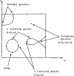
More precisely, the entire algebraic surface f(r) = 0 does not intersect the surface patch r = r(u, v) for (u, v) ∈ [0,1]2. Obviously, when all cBij=0 the two surfaces coincide in their entirety. A somewhat complex algebraic curve F(u, v) = 0 is shown in Figure 25.1 involving various branches (from border to border), internal loops, and singularities.
Tracing method
Given a point on every branch of an algebraic curve, the curve can be traced using differential curve properties. We now consider the intersection curve which lies on the surface represented by the parametric form r(t) = r(u(t), v(t)). Differentiating (25.26) with respect to t yields
where u, v are considered as functions of a parameter t. The solution to the differential equation is given by
where ξ is an arbitrary nonzero factor. For example, ξ can be chosen to provide arc length parametrization using the first fundamental form of the surface as a normalization condition
where E, F and G are first fundamental form coefficients of the parametric surface following standard differential geometry terminology. Note that F in Equation (25.29) has no relation with function F that appears in Sections 25.4 and 25.5. Equations (25.28) form a system of two first order nonlinear differential equations which can be solved by the Runge-Kutta or other methods with adaptive step size [15]. For a tracing method to work properly, we must provide all the starting points of all branches in advance. Step size selection is complex and too large a step size may lead to straying or looping. Tracing through singularities (F2u+F2v=0) is also problematic.
Characteristic points
Starting points for tracing algebraic curves are identified by looking for characteristic points defined below:
1. Border points: The intersections of F(u, v) = 0 with all four boundary edges of the parameter space [0,1]2, e.g. F(0, v) =0, 0 ≤ v ≤ 1.
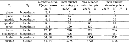
2. Turning points: The u-turning points are the points where the tangent of F(u, v) = 0 is parallel to the u = 0 axis, which satisfies the simultaneous equations F = Fv = 0 (with Fu ≠ 0). On the other hand the v-turning points are the points where the tangent of F(u, v) = 0 is parallel the v = 0 axis, which satisfies the simultaneous equations F = Fu = 0 (with Fv ≠ 0). Both types of turning points are shown in Fig. 25.1. If F has a degree of (M, N) in (u, v), then the degrees of Fu and Fv will be (M − 1, N) and (M, N − 1), respectively. It can be shown that the total number of roots of two simultaneous polynomial equations in two variables whose degree are(m, n) and (p, q), respectively, is mq + np [19]. Therefore the number of u-turning points and v-turning points can be at most 2MN - M and 2MN - N, respectively.
3. Singular points: The points on the curve which satisfy the following three simultaneous equations F = Fu = Fv = 0 are called singular points. Noting that f(x, y, z) = 0, and F(u, v) = Wm(u, v)f(x, y, z) = 0, we deduce
and hence at singular points ∇f ˙ ru = ∇f ˙ = 0. This means that ∇f || ru × rv or that the normals of two surfaces are parallel and since F(u, v) = 0 at these points the two surfaces intersect tangentially. If F has a degree of (M, N) in (u, v), the degrees of Fu and Fv will be (M − 1, N) and (M, N − 1), respectively, thus the number of singular points can be at most 2MN - M - N + 1 [19]. However, singular points require little additional computation, since they are merely common roots of the u-turning points and v-turning points.
From the above discussions we can get upper bounds for the maximum number of u-, v-turning points and singular points [68] as listed in Table 25.1. These bounds refer to the maximum possible number of solutions (u, v) in the entire complex plane. Biquadratic and bicubic surfaces in the first colum of Table 25.1 are degree 8 and 18 implicit algebraic surfaces. It turns out that the number of such points in the real square [0,1]2 is much smaller, but can still be quite large. Consequently methods which focus only on the real solutions in [0,1]2 are advantageous, such as the IPP algorithm described in section 25.3.
Analysis of singular points
Let us construct a parametric equation of a straight line L through a point (u0, v0) on the algebraic curve F(u, v) = 0
where α and β are constants and t is the parameter [80],[96]. We find its intersections between L and the algebraic curve F(u, v) = 0 by determining the roots of F(u0 + αt, v0 + βt) = 0. Taylor expansion of the left hand side gives
where partial derivatives of F are evaluated at (u0, v0) and F(u0, v0) = 0 is used.
When Fu and Fv are not both zero (F2u+F2v>0) at (u0, v0), (25.32) has a single root t = 0 and every line through (u0, v0) has a single intersection with the algebraic curve at (u0, v0) except for one case where αFu + βFv = 0 for certain values of α and β. In such cases (25.32) has a double root t = 0, provided at least one of the second order partial derivatives is not zero (F2uu+F2vv>0), and L is tangent to the curve at (u0, v0).
When (u0, v0) is a singular point (Fu(u0, v0) = Fv(u0, v0) = F(u0, v0) = 0), and at least one of Fuu, Fuv, Fvv is not zero ![]() , then t = 0 is a double root and has at least two intersections at (u0, v0) except for the values of α and β which satisfy
, then t = 0 is a double root and has at least two intersections at (u0, v0) except for the values of α and β which satisfy
In such cases, t = 0 is a triple root, provided at least one of the third order partial derivatives is not zero ![]() . We can solve the quadratic equation (25.33) for
. We can solve the quadratic equation (25.33) for ![]() which leads to the following three possibilities: (1) Two real distinct roots: These values correspond to two distinct tangent directions at the singular point, which implies the algebraic curve has a self-intersection. (2) One real double root: This value corresponds to one tangent direction at the singular point, which implies a cusp. (3) Two complex roots: No real tangents at the singular point implies an isolated point.
which leads to the following three possibilities: (1) Two real distinct roots: These values correspond to two distinct tangent directions at the singular point, which implies the algebraic curve has a self-intersection. (2) One real double root: This value corresponds to one tangent direction at the singular point, which implies a cusp. (3) Two complex roots: No real tangents at the singular point implies an isolated point.
Computing starting points for all branches
Starting points for tracing algebraic curves could be border points, turning points and singular points. Border points involve solution of a univariate polynomial equation, e.g. for border along u = 0, using (25.26)
Turning and singular point computation involve the first order partial derivatives:
Consequently, computing turning points (F = Fu = 0 and F = Fv = 0) is equivalent to solving a system of two nonlinear polynomial equations in two variables, and computing singularities F = Fu = Fv = 0 is equivalent to solving an overconstrained system of three nonlinear polynomial equations in two variables. Solution of these nonlinear polynomial systems is addressed in section 25.3.
25.5.2 RPP/RPP surface intersection
Rational polynomial parametric surface to rational polynomial parametric surface intersection is defined as:
Formulation can be provided by setting r1(σ, t) = r2(u, v) which leads to three nonlinear polynomial equations for four unknowns σ, t, u, v. It is an underconstrained system with 3 equations and 4 unknowns. This system can be solved by the IPP algorithm of section 25.3. However, as the solutions are typically not isolated points but curves, such approach is inefficient when small tolerances are used. Another method involves implicitization of r1(σ, t) to the form f(r) = 0 and substitution of r = r2(u, v) into f to reduce the problem to RPP/IA case for a low degree surface [42]. Heo et al. [30] developed an intersection algorithm for two ruled surfaces which performs more efficiently than those for general parametric surfaces.
There are three major techniques for solving RPR/RPP surface intersections. A review as of 1993 can be found in [67] and a more up-to-date and detailed treatment in [68].
Lattice methods
Lattice method reduces the dimensionality of surface intersections by computing intersections of a number of isoparametric curves of one surface with the other surface followed by connection of the resulting discrete intersection points to form different solution branches [75]. For intersections of parametric patches, the method reduces to the solution of a large number of independent systems of nonlinear equations. The reduction of problem dimensionality in lattice methods involves an initial choice of grid resolution, which, in turn, may lead the method to miss important features of the solution, such as small loops and isolated points which reflect near tangency or tangency of intersecting surfaces, and to provide incorrect connectivity. Appropriate methods for the solution of the resulting nonlinear equations in the present context are identified in section 25.3.
Subdivision methods
Subdivision methods in their most basic form, involve recursive decomposition of the problem into simpler similar problems until a level of simplicity is reached, which allows simple direct solution, (e.g. plane/plane intersection). This is followed by a connection phase of the individual solutions to form the complete solution. Initially conceived in the context of intersections of polynomial parametric surfaces [45], they can be extended to the computation of RPP/IA and IA/IA surface intersections [69]. A simple subdivision algorithmemploys uniform subdivision which leads to a uniform quadtree data structure [33]. Subdivision techniques do not require starting points as marching methods, an important advantage. General non-uniform subdivision [13] allows selective refinement of the solution providing the basis for an adaptive intersection technique. A disadvantage of subdivision techniques used in the evaluation of the entire intersection set is that, in actual implementations with finite subdivision steps, correct connectivity of solution branches in the vicinity of singular or near-singular points is difficult to guarantee, small loops may be missed (in methods with polyhedral surface approximations) or extraneous loops may be present in the approximation of the solution. Furthermore, if subdivision methods are used for high precision evaluation of the entire intersection set, they lead to data proliferation and are consequently slow, and, therefore, unattractive. There are many applications in CAD/CAM, that require high accuracy, for which pure subdivision methods are impractical. However, adaptive subdivision methods coupled with efficient local techniques to get high accuracy, offer an attractive approach for the computation of characteristic points. These points can then be used in initiating efficient marching methods for tracing intersection curves.
As can be seen from the above review, common problems of intersection methods include the difficulty in handling singularities, surface overlap and efficiently identifying closely spaced features and small loops. These algorithmic difficulties are further compounded by numerical error present in finite precision computations.
Marching methods
Marching methods involve generation of sequences of points of an intersection curve branch by stepping from a given point on the required curve in a direction prescribed by the local differential geometry [3],[5],[40],[101], similar to tracing a planar algebraic curve F(u, v) = 0 in section 25.5.1. However, such methods are by themselves incomplete in that they require starting points for every branch of the solution. In order to identify all connected components of the intersection curve, a set of characteristic points on the intersection curve can be defined. As seen in section 25.5.1, such a set may include border, turning and singular points of the intersection and provides at least one point on any connected intersection segment and identifies all singularities. For RPP/RPP surface intersections a more convenient set of such points sufficient to discover all connected components of the intersection, includes border and collinear normal points between the two surfaces. Collinear normal points provide points inside all intersection loops and all singular points [34].
Border points are points of the intersection at which at least one of the parametric variables σ, t, u, v takes a value equal to the border of the σ-t or u-v parametric domain. To compute border points, a piecewise rational polynomial curve to piecewise rational polynomial surface intersection capability is required, e.g., r1(0, t) = r2(u, v), which we discussed in section 25.4.2.
Sederberg et al. [84] first recognized the importance of collinear normal points in detecting the existence of closed intersection loops in intersection problems of two distinct parametric surface patches. These are points on the two parametric surfaces at which the normal vectors are collinear. Collinear normal points are a subset of parallel normal points first used by [89] in surface intersection loop detection methods.
To simplify the notation, we replace r1(σ, t) by p(σ, t) and r2(u, v) by q(u, v). Then the collinear normal points satisfy the following equations [34]:
Equations (25.38) form a system of four nonlinear polynomial equations that can be solved using the methods of section 25.3 (see also [34] for more details on interval methods coupled with subdivision to solve the system (25.38)). Now we split the patches in (at least) one parametric direction at these collinear normal points. Consequently, starting points are only border points on the boundaries of all subdomains created. Grandine and Klein [26] follow a systematic approach for topology resolution of B-spline surface intersections. In this process, they determine the structure of the intersection curves including closed loops prior to numerical tracing (following a marching method based on numerical integration of a differential algebraic system of equations). Topology resolution in this context relies on an extension of the PP algorithm (see section 25.3.2) to the B-spline case implemented in floating point (with normalization of the equations in the range [−1, 1] and normalization of the knot vector in each subdomain in the range [0,1] at each iteration step of the process to capitalize on the higher density of floating point numbers in this range, thereby improving numerical robustness of the algorithm). An alternate way to detect closed intersection loops is to use topological methods [12],[40],[49],[51],[52],[60],[95],[94]. Also bounding pyramids [39],[86] can be used effectively to assure the nonexistence of closed surface to surface intersection loops. These earlier methods need to be implemented in exact or RIA for robustness.
In order to trace the intersection curve, starting points must be located prior to tracing. An intersection curve branch can be traced if its pre-image starts from the parametric domain boundary in either parameter domain [4]. The marching direction coincides with the tangential direction of the intersection curve c(s) which is perpendicular to the normal vectors of both surfaces. Therefore, the marching direction can be obtained as follows:
where the normalization forces c(s) to be arc length parametrized and
are the normal vectors of p and q, respectively. When the two surfaces intersect tangentially, we cannot use Equation (25.39) since the denominator vanishes. In such cases we must find the marching direction in an alternate way [103].
The intersection curve can also be viewed as a curve on the two intersecting surfaces. A curve σ = σ(s), t = t(s) in the σt-plane defines a curve r = c(s) = p(σ(s), t(s)) on a parametric surface p(σ, t), as well as a curve u = u(s) v = v(s) in the uv-plane defines a curve r = c(s) = q(u(s), v(s)) on a parametric surface q(u, v). We can derive the first derivative of the intersection curve as a curve on the parametric surface using the chain rule:
Since we know the unit tangent vector of the intersection curve from Equation (25.39), we can find σ′ and t′ as well as u′ and v′ by taking the dot product on both sides of the first equation of (25.41) with pσ and pt and the second equation with qu and qv which leads to two linear systems [34]. The solutions are immediately obtained as
where det denotes the determinant (see also [26]).
The points of the intersection curves are computed successively by integrating the initial value problem for a system of nonlinear ordinary differential equations (25.42) and (25.43) using standard numerical techniques [15].
25.5.3 IA/IA surface intersection
Implicit algebraic surface to implicit algebraic surface intersection is defined as follows:
where f, g are polynomial functions. Here we have two equations in three unknowns r. Bajaj et al. [3] developed a marching method for IA/IA surface intersection (as well as for parametric surfaces).
A method for low order f, g is to eliminate one variable (e.g. z) to find projection of intersection curves on the plane of other two variables (e.g. x, y), then trace the algebraic curve and use the inversion algorithm to find z. Intersections of low degree implicit algebraic surfaces are of special interest in the boundary evaluation of the Constructive Solid Geometry models. A more complete analysis of the special intersections of two quadric surfaces can be found in [48],[61],[82],[87],[98].
25.6 CONCLUSION
Some important outstanding issues in the area of intersection problems are summarized below. While solving nonlinear polynomial systems, as a preliminary step in computing characteristic points of surface intersections, it is frequently necessary to deal with solution sets that are not zero-dimensional (e.g. the solution sets are one-dimensional, two-dimensional etc.). Most of the methods experience serious numerical and efficiency difficulties in those cases. Methods to deal effectively with these problems need to be developed, including methods to identify and, if possible, parameterize these higher-dimensional solution sets.
Extension of current intersection methods applied on rational B-spline surfaces, to more general and complex surfaces requires further study. Such surfaces include offset, generalized cylinder (pipe or canal surfaces in particular), blending, and medial surfaces and surfaces arising from the solution of partial differential equations or via recursion techniques (subdivision surfaces, see chapter 12 of this handbook [76]). Intersections of such surfaces with the basic low order algebraic and rational B-spline surfaces, commonlyused in CAD need to be explored. However, a basic element of a solution of many of these problems is the auxiliary variable method described in [32],[54],[68], where the problem is reduced to a higher dimension nonlinear polynomial system. In some cases, recent research has indicated that some special instances of these general surfaces can be exactly expressed as rational polynomial surfaces [50],[53],[56],[73] of higher degree and therefore these problems are reducible at least in principle to the problems addressed in this paper. Further research is needed to implement this idea in a practical setting and examine the relative efficiency of competing approaches.
Investigating the effects of floating point arithmetic on the implementation of intersection algorithms has been an important area for basic research during the last decade. Ways to enhance the precision of intersection computation, to monitor numerical error contamination and alternate means of performing arithmetic, not relying on imprecise floating point computation alone, have been explored in some detail. Researchers in surface intersection problems during the last decade have already obtained a good understanding of robustness problems when employing floating point arithmetic and of methods to mitigate these problems based on normalization of the system [26] and rounded interval arithmetic [34]. However, these methods are not a panacea since they cannot resolve effectively non-zero-dimensional solution sets of nonlinear systems or achieve very high precision in reasonable computation times. A related active problem area has been the rectification of solid models expressed in the boundary representation form, which attempts to resolve intersection inconsistencies in such models and create topologically and geometrically consistent models [70].
As a result of these deficiencies, recent research tends to focus on exact methods involving rational arithmetic [38],[77],[79]. Much research remains to be done in bringing such methods to the CAD practice, generalizing the arithmetic to go beyond rational and algebraic numbers (eg. involving transcendental numbers of trigonometric form), and to explore more efficient alternatives that are generally applicable in low and high degree problems alike. Finally, a general and comprehensive comparison and mapping of the efficiency properties of all available methods for solving nonlinear systems robustly would be valuable as a guide for future research.
1. July Abrams, S.L., Cho, W., Hu, C.-Y., Maekawa, T., Patrikalakis, N.M., Sherbrooke, E.C., Ye, X. Efficient and reliable methods for rounded-interval arithmetic. Computer-Aided Design. 1998;30(8):657–665.
2. Auzinger, W., Stetter, H.J. An elimination algorithm for the computation of zeros of a system of multivariate polynomial equations. In: Agarwal R.P., Chow Y.M., Wilson S.J., eds. Numerical Mathematics, Singapore, 1988, International Series of Numerical Mathematics, Volume 86. Birkhäuser Verlag; 1988:11–30.
3. November Bajaj, C.L., Hoffmann, C.M., Hopcroft, J.E., Lynch, R.E. Tracing surface intersections. Computer Aided Geometric Design. 1988;5(4):285–307.
4. July Barnhill, R.E., Farin, G., Jordan, M., Piper, B.R. Surface/surface intersection. Computer Aided Geometric Design. 1987;4(1–2):3–16.
5. June Barnhill, R.E., Kersey, S.N. A marching method for parametric surface / surface intersection. Computer Aided Geometric Design. 1990;7(1–4):257–280.
6. July Bliek, C. Computer Methods for Design Automation. PhD thesis, Massachusetts Institute of Technology, Cambridge, MA. 1992.
7. Buchberger, B. Ein Algorithmus zum Auffinden der Basiselemente des Restklassenringes nach einem nulldimensionalen Polynomideal. PhD thesis, University of Innsbruck, Innsbruck, Austria. 1965.
8. Buchberger, B. Gröbner bases: An algorithmic method in polynomial ideal theory. In: Bose N.K., ed. Multidimensional Systems Theory: Progress, Directions and Open Problems in Multidimensional Systems. Dordrecht, Holland: D. Reidel Publishing Company; 1985:184–232.
9. Canny, J.F. The Complexity of Robot Motion Planning. MIT Press; 1988.
10. Canny, J.F., Emiris, I.Z. An efficient algorithm for the sparse mixed resultant. In: Cohen G., Mora T., Moreno O., eds. Proceedings of 10th International Symposium, Applied Algebra, Algebraic Algorithms and Error-Correcting Codes. Cambridge, MA: Springer-Verlag; 1993:89–104.
11. Char, B.W.W., Geddes, K.O., Gonnet, G.H., Leong, B.L., Monagan, M.B., Watt, S.M. First Leaves: A Tutorial Introduction to Maple V. Springer-Verlag; 1992.
12. Cheng, K.-P. Using plane vector fields to obtain all the intersection curves of two general surfaces. In: Strasser W., Seidel H., eds. Theory and Practice of Geometric Modeling. Springer-Verlag; 1989:187–204.
13. October Cohen, E., Lyche, T., Riesenfeld, R. Discrete B-splines and subdivision techniques in computer-aided geometric design and computer graphics. Computer Graphics and Image Processing. 1980;14(2):87–111.
14. Collins, G.E., Loos, R. Real zeros of polynomials. In: Buchberger B., Collins G.E., Loos R., eds. Computer Algebra: Symbolic and Algebraic Computation. New York: Springer-Verlag; 1982:83–94.
15. Dahlquist, G., Björck, Å. Numerical Methods. Vienna: Prentice-Hall, Inc.; 1974.
16. Dennis, J.E., Schnabel, R.B. Numerical Methods for Unconstrained Optimization and Nonlinear Equations. Englewood Cliffs, NJ: SIAM; 1996.
17. Emiris, I.Z. Sparse Elimination and Applications in Kinematics. PhD thesis, University of California at Berkeley, Berkeley, CA. 1994.
18. Farin, G. Curves and Surfaces for Computer Aided Geometric Design: A Practical Guide, 3rd edition. Philadelphia: Academic Press; 1993.
19. February Farouki, R.T. The characterization of parametric surface sections. Computer Vision, Graphics and Image Processing. 1986;33(2):209–236.
20. November Farouki, R.T., Rajan, V.T. On the numerical condition of polynomials in Bernstein form. Computer Aided Geometric Design. 1987;4(3):191–216.
21. June Farouki, R.T., Rajan, V.T. Algorithms for polynomials in Bernstein form. Computer Aided Geometric Design. 1988;5(1):1–26.
22. Faugere, J.C., Gianni, P., Lazard, D., Mora, T. Efficient computation of zero-dimensional Gröbner bases by change of ordering. Journal of Symbolic Computation. 1993;16(4):329–344.
23. Garcia, C.B., Zangwill, W.I. Global continuation methods for finding all solutions to polynomial systems of equations in n variables. In: Fiacco A.V., Kortanek K.O., eds. Extremal Methods and Systems Analysis. Boston, MA: Springer-Verlag; 1980:481–497.
24. May Grandine, T.A. Computing zeroes of spline functions. Computer Aided Geometric Design. 1989;6(2):129–136.
25. Grandine, T.A. Geometry processing. In: Farin G., Hoschek J., Kim M.-S., eds. Handbook of Computer Aided Geometric Design. New York, NY: Elsevier, 2002.
26. Grandine, T.A., Klein, F.W. A new approach to the surface intersection problem. Computer Aided Geometric Design. 1997;14(2):111–134.
27. November Hakala, D.G., Hillyard, R.C., Nourse, B.E., Malraison, P.J., Natural quadrics in mechanical design. Proceedings of the Autofact West 1, Anaheim, CA. 1980:363–378.
28. April Van Hentenryck, P., Mcallester, D., Kapur, D. Solving polynomial systems using a branch and prune approach. SIAM Journal on Numerical Analysis. 1997;34(2):797–827.
29. Van Hentenryck, P., Michel, L., Deville, Y. Numerical A Modeling Language for Global Optimization. MIT Press; 1997.
30. January Heo, H.-S., Kim, M.-S., Elber, G. The intersection of two ruled surfaces. Computer-Aided Design. 1999;31(1):33–50.
31. March Hoffmann, C.M. The problems of accuracy and robustness in geometric computation. Computer. 1989;22(3):31–41.
32. November Hoffmann, C.M. A dimensionality paradigm for surface interrogations. Computer Aided Geometric Design. 1990;7(6):517–532.
33. Translated by L.L. Schumaker Hoschek, J., Lasser, D. Fundamentals of Computer Aided Geometric Design. Cambride, MA: A.K. Peters; 1993.
34. September Hu, C.Y., Maekawa, T., Patrikalakis, N.M., Ye, X. Robust interval algorithm for surface intersections. Computer-Aided Design. 1997;29(9):617–627.
35. June/July Hu, C.Y., Maekawa, T., Sherbrooke, E.C., Patrikalakis, N.M. Robust interval algorithm for curve intersections. Computer-Aided Design. 1996;28(6/7):495–506.
36. Jouanolou, J.P. Le formalisme du resultant. Advances in Mathematics. 1991;90(2):117–263.
37. Kearfott, R.B. Interval Newton/generalized bisection when there are singularities near roots. Annals of Operations Research. 1990;25:181–196.
38. September Keyser, J., Culver, T., Manocha, D., Krishnan, S. Efficient and exact manipulation of algebraic points and curves. Computer-Aided Design. 2000;32(11):649–662.
39. Miami, September Kriezis, G.A., Patrikalakis, N.M., Rational polynomial surface intersections [1991] Gabriele G.A., ed. Proceedings of the 17th ASME Design Automation Conference. ASME: Wellesley, MA, 1991:43–53.
40. January Kriezis, G.A., Patrikalakis, N.M., Wolter, F.-E. Topological and differential-equation methods for surface intersections. Computer-Aided Design. 1992;24(1):41–55.
41. December Kriezis, G.A., Prakash, P.V., Patrikalakis, N.M. Method for intersecting algebraic surfaces with rational polynomial patches. Computer-Aided Design. 1990;22(10):645–654.
42. January Krishnan, S., Manocha, D. Efficient surface intersection algorithm based on lower-dimensional formulation. ACM Transactions on Graphics. 1997;16(1):74–106.
43. Lakshman, Y.N. On the complexity of computing Gröbner bases for zero dimensional ideals. PhD thesis, Rennselaer Polytechnic Institute, Troy, NY. 1992.
44. Salt Lake City, Utah, May Lamure, H., Michelucci, D. Solving geometric constraints by homotopy. In: Hoffmann C., Rossignac J., eds. Proceedings of the Third ACM Solid Modeling Symposium. New York: ACM; 1995:263–269.
45. January Lane, J.M., Riesenfeld, R.F. A theoretical development for the computer display and generation of piecewise polynomial surfaces. IEEE Transactions on Pattern Analysis and Machine Intelligence. 1980;2(1):35–46.
46. Lane, J.M., Riesenfeld, R.F. Bounds on a polynomial. BIT: Nordisk Tidskrift for Informations-Behandling. 1981;21(1):112–117.
47. Lazard, D. Solving zero-dimensional algebraic systems. Journal of Symbolic Computation. 1992;13(2):117–131.
48. Levin, J.Z. Mathematical models for determining the intersections of quadric surfaces. Computer Vision, Graphics and Image Processing. 1979;11:73–87.
49. Lloyd, N.G. Degree Theory. NY: Cambridge University Press; 1978.
50. October Lü, W., Pottmann, H. Pipe surfaces with rational spine curve are rational. Computer Aided Geometric Design. 1996;13(7):621–628.
51. December Ma, Y., Lee, Y.-S. Detection of loops and singularities of surface intersections. Computer-Aided Design. 1998;30(14):1059–1067.
52. November Ma, Y., Luo, R.C. Topological method for loop detection of surface intersection problems. Computer-Aided Design. 1995;27(11):811–820.
53. March Maekawa, T. An overview of offset curves and surfaces. Computer-Aided Design. 1999;31(3):165–173.
54. June Maekawa, T., Cho, W., Patrikalakis, N.M. Computation of self-intersections of offsets of Bezier surface patches. Journal of Mechanical Design, Transactions of the ASME. 1997;119(2):275–283.
55. October Maekawa, T., Patrikalakis, N.M. Computation of singularities and intersections of offsets of planar curves. Computer Aided Geometric Design. 1993;10(5):407–429.
56. May Maekawa, T., Patrikalakis, N.M., Sakkalis, T., Yu, G. Analysis and applications of pipe surfaces. Computer Aided Geometric Design. 1998;15(5):437–458.
57. Montreal May 1993 Manocha, D. Solving polynomial systems for curve, surface and solid modeling. In: Rossignac J., Turner J., Allen G., eds. Proceedings of 2nd ACM/IEEE Symposium on Solid Modeling and Applications. New York: ACM Press; 1993:169–178.
58. January 6–7 Manocha, D., Numerical methods for solving polynomial equations. Cox D.A., Sturmfels B., eds., eds. Proceedings of Symposia in Applied Mathematics Volume 53, Applications of Computational Algebraic Geometry: American Mathematical Society short course. 1997. American Mathematical Society: San Diego, California, 1998:41–66.
59. December Manocha, D., Krishnan, S. Solving algebraic systems using matrix computations. Sigsam Bulletin: Communications in Computer Algebra. 1996;30(4):4–21.
60. September Markot, R.P., Magedson, R.L. Solutions of tangential surface and curve intersections. Computer-Aided Design. 1989;21(7):421–429.
61. January Miller, J.R., Goldman, R.N. Geometric algorithms for detecting and calculating all conic sections in the intersection of any two natural quadratic surfaces. Graphical Models and Image Processing. 1995;57(1):55–66.
62. Moore, R.E. Interval Analysis. Prentice-Hall; 1966.
63. July Niizeki, M., Yamaguchi, F. Projectively invariant intersection detections for solid modeling. ACM Transactions on Graphics. 1994;13(3):277–299.
64. August Nishita, T., Sederberg, T.W., Kakimoto, M. Ray tracing trimmed rational surface patches. ACM Computer Graphics. 1990;24(4):337–345.
65. Noro, M., Takeshima, T., Yokoyama, K. Solution of systems of algebraic equations and linear maps on residue class ring. Journal of Symbolic Computation. 1992;14:399–417.
66. Ortega, J.M., Rheinboldt, W.C. Iterative Solution of Nonlinear Equations in Several Variables. Englewood Cliffs, NJ: Academic Press; 1970.
67. January Patrikalakis, N.M. Surface-to-surface intersections. IEEE Computer Graphics and Applications. 1993;13(1):89–95.
68. Patrikalakis, N.M., Maekawa, T. Shape Interrogation for Computer Aided Design and Manufacturing. New York: Springer-Verlag; 2002.
69. March Patrikalakis, N.M., Prakash, P.V. Surface intersections for geometric modeling. Journal of Mechanical Design, Transactions of the ASME. 1990;112(1):100–107.
70. University of Cambridge, UK., September Patrikalakis, N.M., Sakkalis, T., Shen, G. Boundary representation models: Validity and rectification. In: Cipolla R., Martin R., eds. The Mathematics of Surfaces IX. London: Springer; 2000:389–409.
71. Petitjean, S. Algebraic geometry and computer vision: Polynomial systems, real and complex roots. Journal of Mathematical Imaging and Vision. 1999;10(3):191–220.
72. May Piegl, L.A., Tiller, W. Symbolic operators for NURBS. Computer-Aided Design. 1997;29(5):361–368.
73. March Pottmann, H. Rational curves and surfaces with rational offsets. Computer Aided Geometric Design. 1995;12(2):175–192.
74. Pratt, M.J., Geisow, A.D. Surface/surface intersection problems. In: Gregory J.A., ed. The Mathematics of Surfaces. Clarendon Press; 1986:117–142.
75. Rossignac, J.R., Requicha, A.A.G. Piecewise-circular curves for geometric modeling. IBM Journal of Research and Development. 1987;31(3):296–313.
76. Sabin, M. Subdivision surfaces. In: Farin G., Hoschek J., Kim M.-S., eds. Handbook of Computer Aided Geometric Design. Elsevier, 2002.
77. Sakkalis, T. On the zeros of a polynomial vector field. Research Report RC-13303, IBM T. J. Watson Research Center, Yorktown Heights, NY. 1987.
78. June Sakkalis, T. The Euclidean algorithm and the degree of the Gauss map. SIAM Journal on Computing. 1990;19(3):538–543.
79. Sakkalis, T. The topological configuration of a real algebraic curve. Bulletin of the Australian Mathematical Society. 1991;43:37–50.
80. June Sakkalis, T., Farouki, R. Singular points of algebraic curves. Journal of Symbolic Computation. 1990;9:405–421.
81. Samuel, N.M., Requicha, A.A.G., Elkind, S.A. Methodology and results of an industrial part survey. Technical Report Tech. Memo. No. 21, Production Automation Project, University of Rochester, Rochester, NY. 1976.
82. May Sarraga, R.F. Algebraic methods for intersections of quadric surfaces in GMSOLID. Computer Vision, Graphics and Image Processing. 1983;22(2):222–238.
83. October Sederberg, T.W., Anderson, D.C., Goldman, R.N. Implicit representation of parametric curves and surfaces. Computer Vision, Graphics and Image Processing. 1984;28(1):72–84.
84. October Sederberg, T.W., Christiansen, H.N., Katz, S. Improved test for closed loops in surface intersections. Computer-Aided Design. 1989;21(8):505–508.
85. Sederberg, T.W., Zheng, J. Algebraic methods for computer aided geometric design. In: Farin G., Hoschek J., Kim M.-S., eds. Handbook of Computer Aided Geometric Design. Elsevier, 2002.
86. January Sederberg, T.W., Zundel, A.K. Pyramids that bound surface patches. Graphical Models and Image Processing. 1996;58(1):75–81.
87. October Shene, C.-K., Johnstone, J.K. On the lower degree intersections of two natural quadrics. ACM Transactions on Graphics. 1994;13(4):400–424.
88. October Sherbrooke, E.C., Patrikalakis, N.M. Computation of the solutions of nonlinear polynomial systems. Computer Aided Geometric Design. 1993;10(5):379–405.
89. Sinha, P., Klassen, E., Wang, K.K. Exploiting topological and geometric properties for selective subdivision. In: Proceedings of the ACM Symposium on Computational Geometry. New York: ACM; 1985:39–45.
90. Stiller, P. Sparse resultants. Technical Report ISC-96-01-MATH, Texas A & M University, Institute for Scientific Computation. 1996.
91. January 6–7 1997 Sturmfels, B. Introduction to resultants. In: Cox D.A., Sturmfels B., eds. Proceedings of Symposia in Applied Mathematics Volume 53, Applications of Computational Algebraic Geometry: American Mathematical Society short course. San Diego, California: American Mathematical Society; 1998:25–39.
92. January Sturmfels, B., Zelevinsky, A. Multigraded resultants of Sylvester type. Journal of Algebra. 1994;163(1):115–127.
93. December Voelcker, H.B., et al. An introduction to PADL: Characteristics, status, and rationale. Technical Report Tech. Memo. No. 22, Production Automation Project, University of Rochester, Rochester, NY. 1974.
94. December Vrahatis, M.N. CHABIS: A mathematical software package for locating and evaluating roots of systems of nonlinear equations. ACM Transactions on Mathematical Software. 1988;14(4):330–336.
95. December Vrahatis, M.N. Solving systems of nonlinear equations using the nonzero value of the topological degree. ACM Transactions on Mathematical Software. 1988;14(4):312–329.
96. Walker, R.J. Algebraic Curves. Princeton University Press; 1950.
97. July Wilf, H.S. A global bisection algorithm for computing the zeros of polynomials in the complex plane. Journal of the Association for Computing Machinery. 1978;25(3):415–420.
98. October Wilf, I., Manor, Y. Quadric-surface intersection curves: shape and structure. Computer-Aided Design. 1993;25(10):633–643.
99. Winkler, F. Polynomial Algorithms in Computer Algebra. Princeton, New Jersey: Springer-Verlag; 1996.
100. Wolfram, S. The Mathematica Book, 3rd edition. New York: Wolfram Media; 1996.
101. May Wu, S.-T., Andrade, L.N. Marching along a regular surface/surface intersection with circular steps. Computer Aided Geometric Design. 1999;16(4):249–268.
102. Yamaguchi, F. A shift of playground for geometric processing from Euclidean to homogeneous. The Visual Computer. 1998;14(7):315–327.
103. September Ye, X., Maekawa, T. Differential geometry of intersection curves of two surfaces. Computer Aided Geometric Design. 1999;16(8):767–788.
104. Zangwill, W.I., Garcia, C.B. Pathways to Solutions, Fixed Points, and Equilibria. Champaign, IL: Prentice-Hall; 1981.