Gerald Farin

1.1 INTRODUCTION

The term CAGD was coined by R. Barnhill and R. Riesenfeld in 1974 when they organized a conference on that topic at the University of Utah. That conference brought together researchers from the U.S. and from Europe and may be regarded as the founding event of the field. It resulted in the widely influential proceedings [8]. The first textbook, “Computational Geometry for Design and Manufacture” by I. Faux and M. Pratt [63], appeared in 1979. The journal “Computer Aided Geometric Design” was founded in 1984 by R. Barnhill and W. Boehm. Its cover is shown in Figure.1.1.

Another early conference was one held in Paris in 1971. It focussed on automotive design and was organized by P. Bézier, then president of the Societé des I n génieurs de l′Automobile. The proceedings were published by the journal “I n génieurs de l′Automobile.”

A series of workshops started in 1982 at the Mathematics Research Institute at Oberwolfach; these were organized by R. Barnhill, W. Boehm, and J. Hoschek. Ten years later, a parallel development started at the Computer Science Research Institute Schloss Dagstuhl initiated by H. Hagen. In the U.S, a conference series was organized by SIAM (Society for Industrial and Apllied Mathematics); the first one being held 1983 at Troy, N.Y., and organized by H. McLaughlin. In the U.K., the conference series “Mathematics of Surfaces” was initiated by the IMA (Institute for Mathematics and Applications). A Norwegian/French counterpart was started by L. Schumaker, T. Lyche, and P.-J. Laurent.

1.2 EARLY DEVELOPMENTS

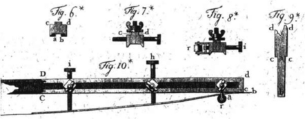
The earliest recorded use of curves in a manufacturing environment seems to go back to early AD Roman times, for the purpose of shipbuilding. A ship’s ribs - wooden planks emanating from the keel - were produced based on templates which could be reused many times. Thus a vessel’s basic geometry could be stored and did not have to be recreated every time. These techniques were perfected by the Venetians from the 13th to the 16th century. The form of the ribs was defined in terms of tangent continuous circular arcs - NURBS in modern parlance. The ship hull was obtained by varying the ribs′ shapes along the the keel, an early manifestation of today’s tensor product surface definitions. No drawings existed to define a ship hull; these became popular in England in the 1600s. The classical “spline,” a wooden beam which is used to draw smooth curves, was probably invented then. The earliest available mention of a “spline” seems to be [51] from 1752. This “shipbuilding connection,” described by H. Nowacki [103], was the earliest use of constructive geometry to define free-form shapes, see Figure.1.2. More modern developments linking marine and CAGD techniques may be found in [10],[100],[115],[136].

Another key event originated in aeronautics. In 1944, R. Liming wrote a book entitled “Analytical Geometry with Application to Aircraft” [95]. Liming worked for the NAA (North American Aviation) during World War II; this company built fighter planes such as the legendary Mustang. In his book, classical drafting methods were combined with computational techniques for the first time. Conics were used in the aircraft as well as in the shipbuilding industries before, essentially based on constructions going back to Pascal and Monge. Traditionally, these constructions found their way onto the draftsman’s drawing board in the form of blueprints which served as the basic product definition. Liming realized that an alternative was more efficient: store a design in terms of numbers instead of manually traced curves. Thus he translated the classical drafting constructions into numerical algorithms. The advantage: numbers can be stored in unambiguous tables and leave no room to individual interpretations of drawings. Liming’s work was very influential in the 1950s when it was widely adopted by U.S. aircraft companies. Figure.1.3 shows one of Liming’s constructions. Another researcher was also involved in the transition of aircraft drawings to computations; this was S. Coons, see [34]. Coons later gained fame for his work at MIT.

Another early influential development for CAGD was the advent of numerical control (NC) in the 1950s. Early computers were capable of generating numerical instructions which drove milling machines used for the production of dies and stamps for sheet metal parts. At MIT, the APT programming language was developed for this purpose. A problem remained: all relevant information was stored in the form of blueprints,¹ and it was not clear how to communicate that information to the computer which was driving a milling machine. Digitizing points off the blueprints and fitting curves using familiar techniques such as Lagrange interpolation failed early on. New blueprint-to-computer concepts were needed. In France, de Casteljau and Bézier went far beyond that task by enabling designers to abandon the manual blueprint process all together.

In the U.S., J. Ferguson at Boeing and S. Coons at MIT provided alternative techniques. General Motors developed its first CAD/CAM system DAC-I (Design Augmented by Computer). It used the fundamental curve and surface techniques developed at GM by researchers such as C. de Boor and W. Gordon.

In the U.K., A.R. Forrest began his work on curves and surfaces after being exposed to S. Coons′ ideas. His PhD thesis (Cambridge) includes work on shape classification of cubics, rational cubics, and generalizations of Coons patches [65]. M. Sabin worked for British Aircraft Corporation and was instrumental in developing the CAD system “Numerical Master Geometry.” He developed many algorithms that were later “reinvented.” This includes work on offsets [118], geometric continuity [116], or tension splines [119]. Sabin received his PhD from the Hungarian Academy of Sciences in 1977, a seemingly odd choice which is explained by the close collaboration between researchers in Cambridge, U.K, and their counterparts in Hungary, under the leadership of J. Hatvany.

All these approaches took place in the 1960s. For quite a while, they existed in isolation until the seventies started to see a confluence of different research approaches, culminating in the creation of a new discipline, CAGD.

Without the advent of computers, a disciplines such as CAGD would not have emerged. The initial main use of these computers was not so much to compute complex shapes but simply to produce the information necessary to drive milling machines. That information was typically output to a punch tape by a main frame computer. That tape was then transferred to the control unit of a milling machine.

The main interest of a designer was not so much the milling machine; it was rather a plotter which could quickly graph a designer’s concepts. Early plotters were the size of a billiard table or larger; this was natural as drawings for most automotive parts were produced to scale. Plotting, or drafting, was so important that almost all of CAD was aimed at producing drawings - in fact, CAD was often considered to stand for “Computer Aided Drafting” (or “Draughting,” in British English). Before the advent of these systems, trivial-sounding tasks were extremely time consuming. For example, producing a new view of a complex wireframe object from existing views would take a draftsman a week or more; using computers, it became a matter of seconds.

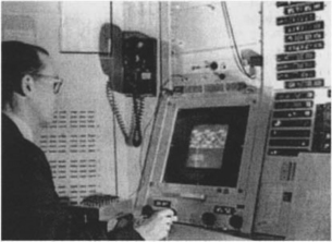
A milestone in display hardware was the use of CRTs, or Cathode Ray Terminals. These went back to oscillographs which were used for many scientific applications. CRTs (not in use for CAD applications any more) displayed an image by “drawing” curves on a screen. Another dimension was added to simple display technology by adding an interactive component to it. The first interactive graphics system was invented by I. Sutherland at MIT in 1963, see [134]. His thesis was part of the CAD project at MIT; S. Coons was a member of his PhD committee. See Figure.1.4 for an illustration of Sutherland’s prototype.

1.3 DE CASTELJAU AND BÉZIER

In 1959, the French car company Citroën hired a young mathematician in order to resolve some of the theoretical problems that arose from the blueprint-to-computer challenge.

The mathematician was Paul de Faget de Casteljau, who had just finished his PhD. He began to develop a system which primarily aimed at the ab initio design of curves and surfaces instead of focusing on the reproduction of existing blueprints.

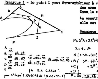
He adopted the use of Bernstein polynomials for his curve and surface definitions from the very beginning, together with what is now known as the de Casteljau algorithm. Figure.1.5 shows a part of his 1963 technical report [44].

The breakthrough insight was to use control polygons (courbes à p^Cles), a technique that was never used before. Instead of defining a curve (or surface) through points on it, a control polygon utilizes points near it. Instead of changing the curve (surface) directly, one changes the control polygon, and the curve (surface) follows in a very intuitive way. In the area of differential geometry, concepts similar to control polygons were devised as early as 1923, see [17], but had no impact on any applications.

De Casteljau’s work was kept a secret by Citroën for a long time. The first public mention of the algorithm (although not including a mention of the inventor) is [93]. W. Boehm was the first to give de Casteljau recognition for his work in the research community. He found out about de Casteljau’s technical reports and coined the term “de Casteljau algorithm” in the late seventies.

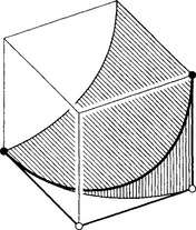
Another place to learn about Citroën’s CAGD efforts was its competitor Rénault, also located in Paris. There, during the early 1960s, Pierre Bézier headed the design department and also realized the need for computer representations of mechanical parts. Bézier’s efforts were influenced by the knowledge of similar developments at Citroën, but he proceeded in an independent manner. Bézier’s initial idea was to represent a “basic curve” as the intersection of two elliptic cylinders, see Figure.1.6. The two cylinders were defined inside a parallelepiped. Affine transformations of this parallelepiped would then result in affine transformations of the curve. Later, Bézier moved to polynomial formulations of this initial concept and also extended it to higher degrees. The result turned out to be identical to de Casteljau’s curves, only the mathematics involved was different. A member of Bézier’s team, D. Vernet independently developed the de Casteljau algorithm. See also Bézier’s chapter in [59].

Bézier’s work was widely published, see [15],[12–14],[138], and soon came to the attention of A.R. Forrest. He realized that Bézier curves could be expressed in terms of Bernstein polynomials - i.e., in the form that de Casteljau had used since the late fifties! Forrest’s article on Bézier curves [66] was very influential and helped popularize Bézier curves considerably. The Rénault CAD/CAM system UNISURF was based entirely on Bézier curves and surfaces. It influenced developments by the French aircraft company Dassault who built a system called EVE. Later, that system evolved into CATIA (Computer Aided Three-dimensional Interactive Application). Bézier also invented a method to deform whole assemblies of surfaces by embedding them into a cube and then deforming it using trivariate “Bézier cubes,” see [12],[16] and Section 1.5.

De Casteljau retired from Citroën in 1989 and became active in publishing. In 1985, he wrote “Formes á P^Cles,” [45] which introduced the concept of blossoming. ²

P. Bézier died in Paris in 1999.

1.4 PARAMETRIC CURVES

Curves were employed by draftsmen for centuries; the majority of these curves were circles, but some were “free-form.” Those are curves arising from applications such as ship hull design to architecture. When they had to be drawn exactly, the most common tool was a set of templates known as French curves. These are carefully designed wooden curves and consist of pieces of conics and spirals. A curve is drawn in a piecewise manner by tracing appropriate parts of a French curve.

Another mechanical tool, called a spline was also used. This was a flexible strip of wood that was held in place and shape by metal weights, known as ducks. When drawings had to be produced to scale, the attics (or lofts) of buildings were used to accommodate the large size drawings - the word lofting has its origins here. A spline “tries” to bend as little as possible, resulting in shapes which are both aesthetically pleasing and physically optimal. The mathematical counterpart to a mechanical spline is a spline curve, one of the most fundamental parametric curve forms.

The differential geometry of parametric curves was well understood since the late 1800s after work by Serret/Frenet. On the other hand, research in approximation theory and numerical analysis focused entirely on nonparametric functions. Both areas were brought together when they became important building blocks of CAGD.

Since the middle 1950s, the US aircraft company Boeing employed software based on Liming’s conic constructions in the design of airplane fuselages. In a different part of the company, J. Ferguson and D. MacLaren developed a different kind of curve for the design of wings. They had the idea to piece cubic space curves together so that they formed composite curves which were overall twice differentiable [97],[64]. These curves could easily interpolate to a set of points. They were referred to as spline curves since they minimize a functional similar to the physical properties of mechanical splines.

The meaning of the term “spline curve” has since undergone a subtle change. Instead of referring to curves that minimize certain functionals, spline curves are now mostly thought of as piecewise polynomial (or rational polynomial) curves with certain smoothness properties.

Ferguson derived his spline equations using the piecewise monomial form. But he also used the cubic Hermite form (then referred to as F-curves) which defines a cubic in terms of two endpoints and two endpoint derivatives. S. Coons used this curve type to build the patches which were named after him. In the UK, A.R. Forrest continued Coons′ ideas and extended cubic Hermite curves to rational cubics, see [65].

The most fundamental parametric curve form are the Bézier curves; see Section 1.3.

Many of the basic properties can be found in the papers by Bézier, Vernet, and Forrest (see above). Some later results include conditions for C^r joins between Bézier curves, see Stärk [131], the discovery that Bézier curves are numerically more stable than other curve forms, see Farouki/Rajan [62], and the development of the blossoming principle, see Ramshaw [110] and de Casteljau [46]. A symbolic technique for Bézier curves and surfaces was developed by M. Hosaka and F. Kimura [83], although it was known to W. Boehm in 1972.³

As an early alternative to parametric curves were explicit curve segments with individual local coordinate systems. These curves are known as Wilson-Fowler splines [68]. A similar curve type was employed in the TABCYL (TABulated CYLinder) routines of the APT (Automatic Programmed Tool) language. After the advent of parametric curves, these piecewise explicit curves began to disappear.

Another early curve scheme are biarcs. These are piecewise circular arcs which are pieced together to allow for tangent continuity. It is possible to fit two tangent continuous circles to two points and two tangents. If several points and tangents are given, one obtains a circle spline. The advantage of these curves is the fact that NC machines can process circular arcs directly, i.e., without a conversion to a dense polygon as is needed for standard parametric splines. A drawback of circle splines is their piecewise constant and hence discontinuous curvature. The first developments are due to K. Bolton [23], followed by M. Sabin [121]; a generalization to 3D was given by T. Sharrock [127].

1.5 RECTANGULAR SURFACES

Parametric surfaces were well understood after early work by Gauss and Euler. They were immediately adopted in early CAD/CAM developments: A standard application is tracing a surface for plotting or for driving a milling tool. Parametric surfaces are well-suited for both tasks. The most popular of all surface methods was to become the tensor product surface. It was first introduced by C. de Boor [39] for the case of bicubic spline interpolation. Theoretical studies of parametric surfaces for the purpose of interpolation and approximation go back to [33],[88],[87],[135],[122],[132] but had little influence on the development of industrial methods.

In the late 1950s, parametric surfaces were studied at several companies in Europe and the U.S. The first published result is due to J. Ferguson at Boeing, see [64]. Ferguson used an array of bicubic patches which interpolated to a grid of data points. While Ferguson developed C² cubic spline curves in the same paper, his surfaces were only C¹.⁴ This was due to the introduction of zero twists at the corner of every bicubic patch. ⁵ Ferguson’s bicubic patches were also known as F-patches, and were also attributed to S. Coons.

Coons devised a simple formula to fit a patch between any four arbitrary boundary curves [35], known as the bilinearly blended Coons patch. These surfaces were used in the sixties by Ford (Coons was a consultant). A generalization, capable of interpolating a rectangular network of curves, was devised by W. Gordon at General Motors, see [71],[72]. All these methods are sometimes labeled “transfinite interpolation,” in that they interpolate to arbitrary boundary curves (having a “transfinite” number of points on them).

While the basic Coons patch had no restrictions on the boundary curves other than they have to meet at the patch corners, a common use was to restrict the boundary curves to be parametric cubics in Hermite form. Then the use of zero corner twists led to the above F-patch.

The basic (bilinearly blended) Coons patch does not lend itself to the construction of composite smooth surfaces. Additions to the basic method led to the bicubically blended Coons patch. It is the generalization of cubic Hermite curve interpolation to the transfinite surface case and allows for the prescription of tangent data in addition to the boundary curves. As a consequence, certain incompatible situations could arise. J. Gregory was the first to address this problem and also to devise a “compatibly corrected” interpolant, see [77]. When applied to cubic boundary curves and cubic derivative information, this interpolant yields a rational patch. A “translation” of this approach into a Bézier-like form was carried out by H. Chiyokura and F. Kimura [29],[28]. It led to the Japanese CAD/CAM system DESIGNBASE.

Rectangular surfaces are a map of a rectangular domain into 3D. As a special case, we may map the domain to a 2D parametric surface, resulting in a distortion of the domain rectangle. If we embed a curve in this domain rectangle, we will obtain a deformed curve. A 3D surface may be embedded inside a 3D cube. This cube may be distorted using trivariate polynomials, resulting in a deformed surface. Such deformations are useful if global shape changes in a surface are wanted which would be too tedious to describe in terms of moving control points. The first mention of these volume deformations appears to be in J. Ferguson’s article [64], although no applications are given. Coons was also aware of the possibility of trivariate volumes, see [35]. The first practical use is due to Bézier who described how to use volume deformations in car design [16]. Volume deformations in Bézier form were rediscovered by Sederberg and Parry [126], who used them in a graphics environment.

1.6 B-SPLINE CURVES AND NURBS

B-splines (short for Basis Splines) go back to I. Schoenberg who introduced them in 1946 [123] for the case of uniform knots. B-splines over nonuniform knots go back to a review article by H. Curry in 1947 [38]. In 1960, C. de Boor started to work for the General Motors Research labs and began using B-splines as a tool for geometry representation. He later became one of the most influential proponents of B-splines in approximation theory. The recursive evaluation of B-spline curves is due to him and is now known as the de Boor algorithm [40].

It is based on a recursion for B-splines which was independently discovered by de Boor, L. Mansfield, and M. Cox [37]. It was this recursion that made B-splines a truly viable tool in CAGD. Before its discovery, B-splines were defined using a tedious divided difference approach which was numerically very unstable. For a detailed discussion, see [42].

Spline functions are important in approximation theory, but in CAGD, parametric spline curves are much more important. These were introduced in 1974 by R. Riesenfeld and W. Gordon [73] (the paper is a synopsis of Riesenfeld’s PhD thesis [112]) who realized that de Boor’s recursive B-spline evaluation was the natural generalization of the de Casteljau algorithm. B-spline curves include Bézier curves as a proper subset and soon became a core technique of almost all CAD systems. A first B-spline-to-Bézier conversion was found by W. Boehm [19]. Several algorithms were soon developed that simplified the mathematical treatment of B-spline curves; these include Boehm’s knot insertion algorithm [20], the Oslo algorithm by E. Cohen, T. Lyche, and R. Riesenfeld [32], and the introduction of the blossoming principle by L. Ramshaw [110] and P. de Casteljau [45].

The generalization of B-spline curves to NURBS - Nonuniform rational B-splineS - has become the standard curve and surface form in the CAD/CAM industry. They offer a unified representation of spline and conic geometries: every conic as well as every spline allows a piecewise rational polynomial representation. The origin of the term NURBS is unclear; but the term was certainly a bad choice: it explicitly excludes the popular uniform B-spline curves. The first systematic NURB treatment goes back to K. Versprille’s PhD thesis [139]. Versprille was a student of S. Coons′ who started working with rational curves in the sixties [36]. Coons′ work on rational curves also influenced A.R. Forrest, who wrote his PhD thesis in 1968 [65].

Versprille based rational curves and surfaces in homogeneous (or projective) space. This kind of geometry had already gained importance in the graphics community because of the widespread use of central projections, see Riesenfeld [114].

The development at Boeing is exemplary for the emergence of NURBS. The company realized that different departments employed different kinds of geometry software; worse, those geometries were incompatible. The Liming-based conic software produced elliptic arcs which could not directly be imported into the Ferguson-based spline system and vice-versa. Thus NURBS were adopted as a standard since they would allow a unified geometry representation. ⁶ Companies such as Boeing, SDRC, or Unigraphics (Verspille’s first employer) soon initiated making NURBS an IGES⁷ standard.

A special case of NURBS is given by rational Bézier curves. Even more specialized are conic sections, or rational quadratic Bézier curves. Their treatment goes back to Forrest’s PhD thesis [65]. A rational generalization of the de Casteljau algorithm was fiven by G. Farin [57] in 1983; a (dual) projective formulation was discovered by J. Hoschek [84].

1.7 TRIANGULAR PATCHES

There are (at least) two ways to describe a bivariate polynomial surface. One is as a tensor product, using a rectangular domain. The other one is to write it in terms of barycentric coordinates with respect to a triangular domain. Both methods are outlined in the chapter on Bézier Techniques.

While tensor product surfaces are far more often encountered, triangular ones have been around for a long time also. The first uses of these surfaces goes back to Finite Elements, where they are referred to as “elements.” The simplest type is the linear element, which is simply a planar triangular facet. Its use goes back to the very beginning of Ritz-Galerkin methods. Higher order elements use C¹ quintic elements [92] or C¹ split triangle cubic elements. The latter one, devised by Clough and Tocher as a finite element [31], gained some popularity in the context of scattered data interpolation, see [58].

From a historical perspective, it interesting to observe that early finite element research on triangular patches did not make use of the elegant formalism offered by the use of barycentric coordinates or the Bernstein-Bézier form. Consequently, those papers were fairly tedious - using barycentric coordinate techniques, many pages of proofs can be reduced to a few lines of geometric arguments about Bézier meshes.

Triangular patches in Bernstein form (called Bézier triangles although Bézier never made any mention of them) are due to P. de Casteljau; however, that work was never published (see above). Since Bézier triangles use trivariate Bernstein polynomials which did exist in approximation theory, several researchers developed concepts that were closely related to Bézier triangles: Stancu [133], Frederickson [69], Sabin [120],[121].

M. Sabin gave conditions for smooth joins between adjacent triangular patches; G. Farin [55] gave conditions for C^r joins. Early research on Bézier triangles focussed on equilateral domain triangles; Farin [56],[58] discussed the case of arbitrarily shaped domain triangles.

Bézier triangles, first conceived by an automotive researcher, found their way into approximation theory in the 1980’s. Spaces of piecewise polynomials over triangulations were studied by L. Schumaker and Alfeld see [1],[2].

Coons-like triangular patches were studied in the US during the 1970’s and 1980’s. See Barnhill et al [4], Barnhill and Gregory [7], or Nielson [102].

1.8 SUBDIVISION SURFACES

At the 1974 CAGD conference at the University of Utah, one of the presenters was the graphics artist G. Chaikin. He presented a curve generation method that did not fit the mold of any of the other methods of the conference. Starting from a closed 2D polygon, and using a process of continual “chopping off corners,” he arrived at a smooth limit curve, see [27]. At the conference, both R. Riesenfeld and M. Sabin argued that Chaikin had invented an iterative way to generate uniform quadratic B-spline curves, see [113].

In 1987, C. de Boor discovered that “corner cutting” generalizations of Chaikin’s algorithm also produce continuous curves [43]. He also pointed out that Chaikin’s algorithm was a special case of a class of algorithms described by G. de Rham much earlier [47],[48]. Similar results were discovered by J. Gregory and R. Q u in 1988 - although that work was only published in 1996, see [78].

Chaikin’s algorithm was the starting point for the initial work on subdivision surfaces, going back to two articles in the no. 6 volume of the journal Computer Aided Design, 1978. They were authored by D. Doo and M. Sabin [50] and E. Catmull and J. Clark [26].

Both papers have a similar flavor. Chaikin’s algorithm can be generalized to tensor product surfaces in a straightforward way. Such surfaces have a rectilinear control mesh, and after analyzing the tensor product algorithm, Doo and Sabin reformulated it such that it could also be applied to control meshes of arbitrary topology. Catmull and Clark first generalized Chaikin’s algorithm to uniform cubic B-spline curves and its tensor product counterpart. Then, they also reformulated it for the case of control meshes of arbitrary topology. Both surface schemes yield smooth (G¹) surfaces. The Doo/Sabin surfaces have a piecewise biquadratic flavor; the Catmull/Clark ones have a piecewise bicubic flavor.

In 1987, C. Loop generalized triangular spline surfaces to a new G¹ subdivision surface type, see [96]. Its input control polygon can be any triangular mesh. Loop’s algorithm is based on a subdivision scheme for so-called box-splines by W. Boehm [21] and H. Prautzsch [108].

All three of the above algorithms produce C¹ (for Doo/Sabin and Loop) or C² (for Catmull/Clark and Loop) surfaces if the control meshes are regular, i.e., rectilinear or regular triangular (all triangle vertices have valence six) for Loop. Where the control meshes do not behave like that, the surfaces will have singular points. These singular points hampered the analysis and practical use of subdivision surfaces. A first attempt at investigating these points was undertaken by D. Storry and A. Ball in 1986, see [3], although there is an eigenvalue analysis of the Doo-Sabin process in the original paper [50]. Subsequently, subdivision surfaces gained more popularity, most notably in the computer animation industry.

Early work on subdivision surfaces focussed on approximating surfaces. In 1987, N. Dyn, J. Gregory, and D. Levin discovered an interpolating subdivision scheme, called the 4-point curve scheme, see [54]. It was generalized to surfaces - to the so-called “butterfly algorithm” - by the same authors in 1990, see [53].

1.9 SCIENTIFIC APPLICATIONS

Many areas of science need to model phenomena for which only a set of discrete measurements is available - an example is a weather map where data are collected at a set of weather stations, but a continuous model of temperature, pressure, etc., is desired. Since the location of the data sites has no structure (such as being on a regular grid), the term “scattered data” was coined. If function values are assigned to these data sites, a scattered data interpolant is a function which assumes the given function values at the data sites. The data sites are typically 2D, but may also be 3D.

A scattered data interpolant is a function which interpolates the given data values and gives reasonable estimates in between. One of the first scattered data interpolants is Shepard’s method, see [74],[5],[128]. It computes the function value at an arbitrary (evaluation) point as a linear combination of all given function values, the coefficients being related to the distance of the data sites to the evaluation point. The method itself is too poorly behaved to be viable on its own, but it was used as an ingredient in other methods (see the above references).

Another approach was taken by R. Hardy [80] in 1971, who generalized the concept of splines to surfaces. His surfaces utilize radial basis functions which are bell-shaped functions (reminiscent of univariate B-splines) with their maxima at the data sites. Hardy’s method was used by many practioners, but it was not known if the method would work in all cases. A proof for this was given by C. Micchelli in 1986 at the Mathematics Research Center in Oberwolfach, Germany.

A different generalization of splines to surfaces is the method of thin plate splines due to J. Duchon [52]. Thin plate splines minimize an “energy functional”, similar to the one that spline curves minimize. While spline curves simulate the behavior of an elastic beam, thin plate splines minimize the behavior of a thin elastic plate.

The U.K. statistician R. Sibson developed a scheme that he called nearest neighbor interpolation. It is based on the concept of Voronoi diagrams, also known as Dirichlet tessellations. Sibson showed that any point in the convex hull of a given set of points may be written as a unique linear combination of its neighbors [129]. If the coefficients of this combination are then used to blend given function values, a scattered data interpolant arises [130]. The interpolant is only C⁰ at the given data points, but it is C¹ otherwise. Uses for this method are in the geosciences as well as in image processing.

1.10 SHAPE

When a designer studied a curve on a full size drawing, he could visually detect shape defects such as “flat spots”, unwanted inflections, etc. A good CAD system would then provide methods to improve the given shape.

As the design process moved away from the drawing board and into computer screens, this visual inspection process was not feasible any more since a full scale drawing was out of the question. The scaled down display offered by the computer did not allow to detect shape imperfections in a direct way. Consequently, computer methods had to be developed that allowed easy assessment of shape.

Among the first published methods are curve hodographs, see [11]. These are the plot of a curve’s first derivative curve. Since differentiation is a roughing process, curve imperfections appear “magnified” in the hodograph.

Hodographs do not display the geometry of the curve alone; they depend on the parametrization as well. A more geometric tool is the curvature plot; it plots the curvature of a curve. Since it involves second order derivatives as well as first order ones, it is also a more sensitive tool. An early paper on the use of curvature plots is by Nutbourne et al. [104].

In unpublished work, curvature plots were used by H. Burchardt at General Motors. After de Boor left the company in 1964, interpolating cubic and quintic spline curves had become a tool of choice. Since they are C², they are also curvature continuous. In many cases, however, this does not guarantee pleasant shape, and so Burchardt developed a proprietary scheme that was shape optimizing. A published version is in [24].

Shape optimization became an important element early on in the development of CAGD. Since interpolating spline curves were known to exhibit unwanted undulations, alternatives were studied, typically involving curvature - see [99],[100],[82],[125].

A different approach is to take an existing curve or surface and inspect its shape: if it is imperfect, apply a fairing procedure. Such methods typically aim at removing noise from either data points or control polygons; early work is reported by J. Kjellander [89], J. Hoschek [86] and Farin et al [60].

A curve which is curvature continuous may not be twice differentiable. This fact, when properly exploited, leads to curve generation schemes which have more degrees of freedom than do “standard” spline curves. The extra degrees of freedom are referred to as shape parameters and the resulting curves are called geometrically continuous or G². Early work on this subject is due to G. Geise [70]. Interpolation schemes based on G² continuity were independently developed by J. Manning [98] and G. Nielson [101] in 1974. Later work on the subject includes B. Barsky’s β-splines [9], W. Boehm’s γ-splines [22], and H. Hagen’s τ-splines [79].

Shape does not only play a vital role in interpolation, but also in approximation. The least squares method is the most widespread approximation scheme. It was used early on in most industries; publications include [81],[106],[142]. The least squares method lends itself to the inclusion of conditions that aim at the shape of the result, not just at the closeness of fit. These conditions are typically the result of minimizing certain functionals (such as minimizing “wiggles”); an influential early example is the “smoothing spline” of Schoenberg and Reinsch, see [124],[111], and also Powell [107].

For curves, curvature is a reliable shape measure. For surfaces, several such measures exist, including Gaussian, mean, or total curvatures. A.R. Forrest [67] was the first to use computer graphics for the interrogation of surface shape using curvatures as texture maps; see Fig. 1.7.

Another important shape measure for surfaces comes from the automotive industry. It is customary to put a car prototype in a showroom where the ceiling is lined with florescent light strips. Their reflections are carefully examined before the prototype is accepted. Early computer simulations of this procedure are reported in [90].

1.11 INFLUENCES AND APPLICATIONS

CAGD emerged through the influence of several areas in the 1950s and 1960s, but interactions with other fields of science and engineering were not limited to those years.

The first text on CAGD goes back to I. Faux and M. Pratt. Its title is “Computational Geometry for Design and Manufacture.” The meaning of the term “Computational Geometry” has since changed; it is used to describe a discipline which is concerned with the complexity of algorithms mostly dealing with discrete geometry. The defining text for this area is the one by Preparata and Shamos [109]. An important area of overlap between CAGD and Computational Geometry is that of triangulation algorithms. These are concerned with finding a set of triangles having a given 2D point set as vertices. The first algorithm was published in 1971 by C. Lawson [94]. An algorithmic connection between triangulations and Voronoi diagrams was presented by Green and Sibson [76]. The n—dimensional case was covered by D. Watson [140].

2D triangulations are an important preprocessing tool for many surface fitting operations. 3D point sets arise when physical objects are digitized. Methods to triangulate them go back to Choi et al. [30].

Computer Graphics is an area with many CAGD interactions. Computer Graphics needs CAGD to model objects to be displayed, and for the very same reason, CAGD needs Computer Graphics. It was only after Sutherland’s 1963 development of interactive graphics that one could interactively change control polygons of Bézier or B-spline objects. Display techniques for parametric surfaces go back to H. Gouraud [75] and were later improved by B. Phong [105] and J. Blinn [18], all at the University of Utah.

A fundamental display technique is ray tracing, due to T. Whitted [141]. It makes extensive use of computations of the intersection between a ray and the scene to be displayed. Hence the development of efficient intersection algorithms became important for Graphics.

Intersection algorithms are also important in many areas of CAD/CAM, where planar sections were the method of choice (and tradition) to display/plot objects. Algorithms for this task were developed by many companies, and were mostly kept confidential. Some early published work is by W. Carlson [25], T. Dokken [49] Barnhill et al [6]. The earliest reference seems to be by M. Sabin [117].

Another important type of numerical algorithms are offset curves and surfaces - early work includes papers by R. Farouki [61], J. Hoschek [85], R. Klass [91], W. Tiller and E. Hanson [137], the earliest one being a technical report by M. Sabin [118] from 1968.

REFERENCES